Copyright1998 by the Genetics Society of America
Statistical Analysis of Ordered Tetrads
Hongyu Zhao* and Terence P. Speed
†*Department of Epidemiology and Public Health, Yale University School of Medicine, New Haven, Connecticut 06520 and†Department of Statistics, University of California, Berkeley, California 94720
Manuscript received January 12, 1998 Accepted for publication May 18, 1998
ABSTRACT
Ordered tetrad data yield information on chromatid interference, chiasma interference, and centromere locations. In this article, we show that the assumption of no chromatid interference imposes certain constraints on multilocus ordered tetrad probabilities. Assuming no chromatid interference, these con-straints can be used to order markers under general chiasma processes. We also derive multilocus tetrad probabilities under a class of chiasma interference models, the chi-square models. Finally, we compare centromere map functions under the chi-square models with map functions proposed in the literature. Results in this article can be applied to order genetic markers and map centromeres using multilocus ordered tetrad data.
G
ENETIC studies using tetrad data are very valuable Papazian(1952) andPerkins(1955), used only threeloci for the detection of chromatid interference and in studying the chance mechanisms in meiosis,
including: (1) positions of crossovers along the four- one locus for mapping centromeres. Several studies
have taken a multilocus approach: (1) under the as-strand bundle; (2) nonsister as-strand pairs involved in
each crossover; (3) spindle-centromere attachment at sumption of no chromatid interference (NCI), Risch
andLange(1983) fitted one class of chiasma
interfer-the first meiotic division; and (4) spindle-centromere
attachment at the second meiotic division. Deviation ence models, the count-location model, to one
multilo-cus unordered tetrad data set; (2)Zhao et al. (1995b)
from random distributions of crossovers on the
four-fitted another class of chiasma interference models, the strand bundle is called chiasma interference. Deviation
chi-square model, to several multilocus unordered tet-from random involvement of nonsister chromatid pairs
rad data sets; and (3) Zhao et al. (1995a) derived a
in each crossover is called chromatid interference.
Com-set of linear equality and inequality constraints on the pared with single spore data, where the four products
probabilities of unordered tetrad patterns, with an arbi-from a single meiosis can only be recovered separately,
trary number of loci under the assumption of NCI, and tetrad data, where four meiotic products can be
recov-tested these constraints on data sets from a variety of ered together, have several advantages. First, chromatid
organisms reported in the literature. interference and chiasma interference can be
distin-In this article, ordered tetrad data are studied under guished using tetrad data. Second, when chromatid
in-different assumptions on the chance mechanisms. For terference is absent, chiasma interference can be
de-each assumption, a detailed discussion is provided for tected with only two markers, whereas at least three
single marker and two marker data. General results markers are needed for single spore data. Chiasma
inter-for multiple markers are then presented. Although the ference can even be detected with one marker in some
number of spores is four in a tetrad and eight in an studies. Third, the position of the centromere can be
octad, there is no loss of generality for discussing only inferred. In some organisms, such as Neurospora crassa,
tetrads when aberrant segregations can be ignored. the asci are produced in a linear order corresponding
Half-tetrad data are another type of genetic data that to the meiotic divisions and are called ordered tetrads.
are closely related to ordered tetrad data and widely In other organisms, such as Saccharomyces cerevisiae, the
used in genetic studies. A detailed study of half-tetrad asci are produced as a group without order and are
data is given in the accompanying article (Zhao and
called unordered tetrads.
Speed1998).
Ordered tetrads have been used extensively to study
We adopt the following notation in this article.
Mark-the crossover process during meiosis sinceLindegren
ers are denoted by script letters; for example, we use (1932, 1933, 1936a,b). However, most studies on
or-A and B to denote markers. Alleles are denoted by
dered tetrads and unordered tetrads, for example,
italic letters. For example, A and a denote two alleles
of markerA. We use [X, Y, Z, W] to denote the observed
marker configuration for an ordered tetrad, where X
Corresponding author: Hongyu Zhao, Department of Epidemiology
and Y are attached to one centromere and Z and W are
and Public Health, Yale University School of Medicine, 60 College
St., New Haven, CT 06520. E-mail: [email protected] attached to the other centromere. For example, [AB,
TABLE 2 TABLE 1
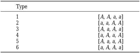
Six possible configurations at markerA Eight ordered tetrad types with the same probability under RSCA
Type
[1, 2, 3, 4]
1 [A, A, a, a] [1, 2, 4, 3]
2 [a, a, A, A] [2, 1, 3, 4]
3 [A, a, A, a] [2, 1, 4, 3]
4 [a, A, a, A] [3, 4, 1, 2]
5 [A, a, a, A] [3, 4, 2, 1]
6 [a, A, A, a] [4, 3, 1, 2]
[4, 3, 2, 1]
Ab, aB, ab] represents an ordered tetrad with two strands
carrying AB and Ab attached to one centromere and
able patterns, the number of distinct probabilities is with two strands carrying aB and ab attached to the
seven under RSCA. These seven groups are shown in other centromere. The centromere is denoted by CEN.
Table 3. When Ashows FDS, there are three distinct
For patterns between a pair of markers, we use P to
groups corresponding to whetherAandBhave
paren-denote parental ditype where all four strands retain the
tal ditype, nonparental ditype, or tetratype, denoted by parental type, T to denote tetratype where two of the
P1, N1, and T12, respectively, in Table 3. WhenAshows
four strands show recombination, and N to denote
non-SDS, there are four distinct groups. Two groups corre-parental ditype where all four strands are recombinants.
spond to Aand Bhaving parental and nonparental
di-types, denoted by P2and N2, respectively, in Table 3. When
METHODS AandBhave tetratype,Bcan show either FDS or SDS.
Under RSCA, these two groups may have different
proba-Random spindle-centromere attachment assumption:
bilities, denoted by T21and T2. RSCA can be tested by
Random spindle-centromere attachment (RSCA) assumes
examining whether all distinguishable patterns within that two centromeres have the same chance to go to
each group occur with equal frequency. For example, the either pole at the first meiotic division, and the divided
8 distinguishable patterns listed above, which correspond centromeres have the same chance to go to either pole
to group T12withAshowing FDS andAandBhaving
at the second meiotic division (Griffithset al. 1996).
tetratype, should occur with equal frequency. These and
For marker A with alleles A and a inherited from
more cases were first studied byWhitehouse(1942).
two parents, there are six distinguishable configuration
For n markers, there are 6ndistinguishable patterns.
types, as illustrated in Table 1. Under RSCA, types 1
Under RSCA, these 6npatterns reduce to (6n 1 5 3
and 2 ([A, A, a, a] and [a, a, A, A]) have the same
2n)/8 distinct probabilities. This result was first derived
probability because of random spindle-centromere
at-byPapazian(1952). In theappendix(Proposition 1),
tachment at the first meiotic division, whereas types 3
we present a different derivation of this result through to 6 ([A, a, A, a], [a, A, a, A], [A, a, a, A], and [a, A,
a more direct counting method. As for the one- and
A, a]) have the same probability because of random
two-marker cases, RSCA can be tested by examining spindle-centromere attachment at the second meiotic
whether all the distinguishable tetrad patterns that division. Types 1 and 2 are called first division
segrega-should have the same probability (as discussed in the tion (FDS) pattern, and types 3 to 6 are called second
proof of Proposition 1 in the appendix) under RSCA
division segregation (SDS) pattern (Griffiths et al.
do occur equally frequently. 1996). For a single marker, RSCA can be tested by
exam-No chromatid interference (one marker):For the case ining whether types 1 and 2 occur with equal frequency
of one marker,A, if NCI holds, the four configurations
and whether types 3, 4, 5, and 6 occur with equal
fre-corresponding to the SDS pattern have the same
proba-quency. RSCA is generally confirmed (Fincham et al.
bility before meiotic divisions. Therefore, these four types 1979).
should occur with the same frequency even if RSCA
For the two markersAandB, there are six
distinguish-fails. As a result, only when both NCI and RSCA fail can
able configurations atA and six distinguishable
con-these four types occur with different probabilities.
figurations atB. Therefore, there are 36 distinguishable
As shown byMather(1935), under NCI, the
proba-patterns jointly at two markers. Under RSCA, if one
bilities that A shows FDS and SDS patterns, given k
pattern can be changed to another pattern through one
chiasmata between CEN andA, are
of the eight permutations in Table 2, these two patterns should have the same probability. For example, the
fol-F(k)
A 5P (FDS|k chiasmata)5 2⁄3(1⁄2 1(21⁄2)k) , (1)
lowing eight types have the same probability: [AB, Ab,
aB, ab], [Ab, AB, aB, ab], [AB, Ab, ab, aB], [Ab, AB, ab, and aB], [aB, ab, AB, Ab], [ab, aB, AB, Ab], [aB, ab, Ab, AB],
and [ab, aB, Ab, AB]. After examining all 36 distinguish- S(k)
TABLE 3
Seven distinct groups under RSCA
B
FDS
SDS
P1 N1 T12
FDS [AB, AB, ab, ab] [Ab, Ab, aB, aB] [AB, Ab, aB, ab]
A
SDS [AB, aB, Ab, ab] [AB, ab, AB, ab] [AB, ab, Ab, aB] [Ab, aB, Ab, aB]
T21 P2 T2 N2
Suppose A/a and B/b are both segregating. The 636536 combinations of ordered tetrads reduce to just 7 under RSCA. P, parental ditype; T, tetratype; N, nonparental ditype.
As k increases, the probability of SDS tends to 2⁄
3. For
p(P(1,1)
2 )5 p(N(1,1)2 )5 1⁄4,
one marker, A, NCI imposes no constraints on the
probabilities of FDS and SDS, denoted by FA and SA. and
For any observed FDS and SDS proportions, we can
p(T(1,1) 2 )51⁄2.
always construct a chiasma process model that gives rise
to the observed FDS and SDS proportions. In fact, the For k1, .2,
process with probability FA having zero chiasmata and p(P(k,,)
1 )5p(N(k,1 ,))51⁄2F(k)AF(B,),
with probability SAhaving one chiasma is the simplest
such model. p(T(k,,)
12 )5F(k)AS(B,), p(T21(k,,))5S(k)AF(B,), No chromatid interference (two markers):Two
mark-p(P(k,,)
2 )5p(N(k,2 ,))51⁄2p(T2(k,,))51⁄4S(k)AS(B,),
ers,AandB, may be (1) on different chromosomes; (2)
on the same chromosome but on different sides of the where F(k)
A and S(k)A were defined in (1). For a given
chi-centromere (that is, the order isA–CEN–B); or (3) on asma process along the four-strand bundle, let ck,denote
the joint probability of there being k chiasmata between the same chromosome and on the same side of the
centro-CEN andAand,chiasmata between CEN andB. The
mere (that is, the order is CEN–A–Bor CEN–B–A). We
above relations can be combined with expressions for study these three cases separately. These three cases
(ck,) and summed, to give our desired frequencies. For
were first discussed in detail by Whitehouse (1942).
example, We use the notation in Table 3 to denote seven distinct
groups. For example, P1is the group with both markers
frequency of P15
o
∞
k50
o
∞,50
ck,p(P(k,1 ,))
showing FDS and no strand showing recombination
be-tween AandB.
and
Two markers on different chromosomes: Let p and q denote
the probability of SDS atAandB. When both markers
frequency of N15
o
∞
k50
o
∞,50
ck,p(N(k,1,)).
have FDS, tetrad types betweenAandBcan be either
parental ditype or nonparental ditype, depending on
On the basis of the above results, it can be shown which pair of alleles are separated at the first meiotic
that, for any chiasma process, seven distinct groups can division—AB vs. ab or Ab vs. aB. The probability of either
have at most five different probabilities: the probabilities
outcome, group P1or N1, is (12p)(1 2q)/2. Similar
of P1, N1, T12, T21, and (P2 1 T2 1 N2) can differ, and
considerations lead to the probabilities of the seven
we denote them by a,b,g,d, and ε. The ratio of the
groups in Table 4. These seven probabilities are
deter-probabilities of P2:T2:N2is 1:2:1. Therefore, the
probabil-mined by two independent parameters: p and q.
ities of P2, T2, and N2areε/4,ε/2, andε/4, respectively.
Two markers on different sides of the centromere (A–CEN–B):
These are summarized in Table 5.
We use p(P(k,,)
1 ), p(N(k,1 ,)), p(T(k,12,)), p(P(k,2,)), p(N(k,2,)),
The probabilities of these seven groups can be derived
p(T(k,,)
21 ), and p(T(k,2 ,)) to denote the frequency of ordered
by another approach. If we treat the centromere as a
tetrads of groups P1, N1, T12, P2, N2, T21, and T2 among
marker, the results for unordered tetrads (Zhao et al.
meioses with k chiasmata inA–CEN and,chiasmata in
1995a) can be applied in this context. If the two
centro-CEN–B. We can easily check that
meres from the two parents could be distinguished,
p(P(0,0)
1 )51, p(T(0,1)12 )5p(T(1,0)21 )51, there would be three types, P, T, and N, betweenAand CEN, and three types, P, T, and N, between CEN and p(P(0,2)
1 )5p(P(2,0)1 )5 p(N(0,2)1 )5p(N(2,0)1 )51⁄4, B
. This would lead to nine distinct probabilities. Let
pk
0, pk1, and pk2 denote the conditional probabilities of
p(T(0,2)
TABLE 4
The probabilities of seven groups whenAandBare on different chromosomes
B
FDS
SDS
P1 N1 T12
FDS 1⁄
2(12p)(12q) 1⁄2(12p)(12q) (12p)q
A
SDS p(12q) 1⁄
4pq 1⁄2pq 1⁄4pq
T21 P2 T2 N2
p and q are SDS proportions atAandB.
pk
0, pk1, and pk2of P, T, and N, given k chiasmata between derive constraints on ordered tetrad probabilities under
NCI. Following the definition in Zhao et al. (1995a),
a pair of markers. Under NCI,Mather(1935) showed
that, for k$ 1, we say a chiasma process is compatible with a given set
of joint tetrad probabilities p if, under NCI, this chiasma
pk
051⁄3(1⁄21(21⁄2)k),
process gives rise to these joint probabilities. It was
shown in Zhao et al. (1995a) that for any underlying
pk
152⁄3(1 2(21⁄2)k), (2)
chiasma process, if NCI holds, there is a chiasma process
pk
251⁄3(1⁄21(21⁄2)k).
with at most two exhanges between each consecutive pair of markers, inducing the same tetrad probabilities.
When k50, p0
05 1 and p015 p0250. Let pijdenote the
probability of joint tetrad pattern (ij), where i, j5 0, Using this property, Zhao et al. (1995a) showed that,
for a given set of unordered tetrad probabilities p 5
1, or 2 corresponding to P, T, and N in each interval;
then, (p0, p1, p2)9, the probabilities of P, T, and N between
two markers, there is some chiasma process compatible
pij 5
o
∞k50
o
∞,50
ck,pkip,j, with p if and only if T211p$0, where
where pk
i and p,j were defined in (2). Because the two
centromeres cannot be distinguished, some of these
T15
1 0 1⁄
4
0 1 1⁄
2
0 0 1⁄
4
, T21
1 5
1 0 21
0 1 22
0 0 4
, classes are not distinguishable. For example, (0, 0) and
(2, 2) both give rise to FDS at two markers and no
recombinations between these two markers. Using the and 0 5 (0, 0, 0)9. For two markers, write the p
ij in
notation in Table 5, we havea 5p(P1)5p001 p22,b 5 lexicographical order as p; there is an underlying
chi-p(N1)5p021p20,g 5p(T12)5p011p21,d 5p(T21)5 asma process satisfying NCI compatible with unordered
p101 p12, andε54p(P2)52p(T2)54p(N2)5p11. tetrad probabilities p if and only if T21
2 p$0, where T25
It was shown inZhaoet al. (1995a) that NCI imposes
T1^T1, T2215 T211^T211and 0 is a column vector with
equality and inequality constraints on the probabilities nine 0’s, plus equality constraints described inZhao
et
of distinguishable unordered tetrad patterns. Here we
al. (1995a). The operator^is the standard tensor
prod-uct (see, e.g., Bellman 1970). If the chiasma process
has at most two chiasmata in each interval, the
corre-TABLE 5
spondence between p and c 5 (ck,) is simply c 5
The probabilities of seven groups whenAandBare
T21
2 p. Using the property that, for any underlying
chi-on different sides of the centromere
asma process, there is a compatible chiasma process with at most two chiasmata in each interval, we may B
focus on the study of chiasma processes with at most
FDS two chiasmata in each interval. Using the notation in
SDS
Table 5, we have the following proposition, whose proof
P1 N1 T12
is given in the appendix(Proposition 2): under NCI,
FDS a b g for any joint ordered tetrad probabilities with two
mark-A
ers on different sides of the centromere, there is an
SDS d 1⁄
4ε 1⁄2ε 1⁄4ε
underlying chiasma process that is compatible with
T21 P2 T2 N2 these probabilities if and only ifa $ bandg 1 d $2b
and the ratios of p(P2):p(T2):p(N2) are 1:2:1.
In the table,a,b,g, d,εall$0,a 1 b 1 g 1 d 1ε51,
TABLE 6 each pair of consecutive markers, there are three types:
P, T, and N. Each of these 23 3n21types can be repre-The probabilities of seven groups whenAandBare on
sented as (i1i2· · · in), where i15 0 or 1 corresponding
one side of the centromere and in the order of CEN–A–B
to FDS or SDS atA1, and ir5 0, 1, or 2 corresponding
to P, T, or N betweenAr21 andAr, for r5 2, . . . , n.
B
For unordered tetrads with n markers (n21 intervals),
FDS
SDS there are 3n21distinct probabilities because FDS and SDS
P1 N1 T12 cannot be differentiated atA1; that is, i1cannot be
deter-mined. Write the probabilities of the observable patterns
FDS a b g
(i2 . . . in) from unordered tetrads, denoted by pti2...in, in A
SDS 1⁄
2φ d 1⁄2φ ε lexicographical order as pt. It was shown that there is an
underlying chiasma process satisfying NCI compatible with
T21 P2 T2 N2
unordered tetrad probabilities if and only if T21
n21pt$0, In the table,a,b,g,d,ε,φ all$0,a 1 b 1 g 1 d 1ε1 where T
n215T1^. . .^T1(n21 terms), plus equality
φ51. The constraints are:a $ b,g $2b,d $ε,φ$2ε.
constraints described inZhao et al. (1995a).
In our discussion of multiple marker ordered tetrad
data, the pt
0i2...inand p
t
1i2...inare considered separately. Write
that A andB show P, T, and N, as p(P) 5 a 1 ε/4,
the pt
0i2...inin lexicographical order as p
t
0, the pt1i2...inin
lex-p(T )5 g 1 d 1ε/2, and p(N)5 b 1ε/4, respectively.
icographical order as pt
1. If for a given (0i2. . . in), there In the unordered tetrad case, the constraints imposed
are k$2 tetratypes in the n21 intervals, these tetratype
by NCI are: p(P )$ P(N ) and p(T )$ 2p(N) (Zhao et
combinations may be subdivided further into 4k21
sub-al. 1995a). Substituting a, b,g,d, andε in these two
cells as follows. First, the strands can be labeled such that
inequalities, we geta $ bandg 1 d $ 2b. Therefore,
strands 1 and 3 always show recombination between two for markers on different sides of the centromere, the
markers that have tetratype closest to the centromere. For only extra constraints added by ordered tetrads are the
the other k 21 intervals showing tetratype,
recombina-1:2:1 proportionality constriants among p(P2), P(T2),
tions can occur on four possible pairs of strands.
There-and p(N2).
fore, there are 4k21 subtypes. The probability of each
Two markers on the same side of the centromere (CEN–A–B;
subcell can be denoted by p0i2...in(h1. . . hk21), where each
the case of CEN–B–Acan be discussed similarly): As in the
previous discussion, we use (i, j) to denote the nine hjis 1, 2, 3, or 4. If for a given (1i2. . . in), there are k$1
distinct groups if the centromere can be treated as a tetratypes in the n21 intervals, these tetratype
combina-marker. Because the centromere cannot be observed, tions may be subdivided further into 2 34k21subcells
(0, 0) and (2, 0) cannot be distinguished. Both (0, 0) as follows. Suppose the first pair of markers showing
and (2, 0) show FDS atAand parental ditype between tetratype from the centromere isAr21andAr. Marker
AandB. Therefore, we have p(P1)5p001p20. Similarly, Ar21must show SDS, because otherwise there must be
p(N1)5p021p22, p(T12)5p011p21, p(P2)5p10, p(N2)5 a tetratype beforeAr21. MarkerArcan show either FDS
p12, and p(T21)5p(T2)5p11/2. Therefore, these seven or SDS. Two types can thus be distinguished, depending
groups can have at most six different probabilities. Each on whetherA
r shows FDS or SDS. The strands can be
of these 23 3 types can be represented as (i1i2), with labeled such that strands 1 and 3 always show
recombina-i150 or 1 corresponding to FDS or SDS atA, and i25 tion betweenAr21andAr. For the other k21 intervals
0, 1, or 2 corresponding to P, T, or N between Aand showing tetratype, recombinations can occur on four
B. Denote these probabilities bya 5p(P1),b 5p(N1), possible pairs of strands. The probability of each subcell
g 5 p(T12), d 5 p(P2), ε5 p(N2), and φ 5 2p(T21)5 can be denoted by p1i
2...in(h0, h1. . . hk21), where h0is 0
2p(T2) (Table 6). It can be shown, as in Zhao et al. or 1 ifA
rshows FDS or SDS, and each hjis 1, 2, 3, or
(1995a), that for joint tetrad probabilities with two
mark-4 for j$1. Using arguments similar to those inZhao
ers on the same side of the centromere, there is a
com-et al. (1995a), it can be shown that there is an underlying
patible chiasma process under NCI if and only if a $
chiasma process satisfying NCI compatible with pt
0and
b,g $2b,d $ε,φ$ 2ε, and p(T21)5 p(T2). pt
1 if and only if T2n211pt0$0, T2n211pt1$ 0, all the subcell No chromatid interference (multiple markers):Here
probabilities pt
0i2...in(h1, . . . , hr) in a cell i2 . . . in with we consider only markers on the same chromosome.
Mark-ir51 for more than one r are equal, and all the subcell
ers on the same side of the centromere and markers on
probabilities pt
1i2...in(h0, h1, . . . , hr) in a cell i2 . . . inwith different sides of the centromere are discussed separately.
ir51 for one ore more r are equal.
Markers on the same side of the centromere: Under the
Markers on different sides of the centromere: Consider
assumption of NCI, there are 233n21distinct
probabili-markers on one side of the centromere in the order of
ties for n markers in the order of CEN–A1–A2– · · · –
CEN–A1–A2– · · · –An1and markers on the other side
An. Each of these 2 3 3n21 classes can be identified as
model is the Poisson process, which imposes no chiasma could be observed, any joint tetrad pattern can be
repre-interference. In this model, the probability of k chias-sented by (i1i2 . . . in1; j1j2. . . jn2), where ir5 0, 1, or 2
mata between CEN and A is e22d(2d)k/k!. Therefore,
corresponding to P, T, or N betweenAr21and Ar, js5
from (1),
0, 1, or 2 corresponding to P, T, or N betweenBs21and
Bs, and A0 and B0 both denote the same centromere.
FA(d)5
o
∞k50
1
e22d(2d )k k !
23
2 3
1
1
21
1
21 2
2
k
24
513(11 2e
23d),
Because the centromere is not observable, both (0i2. . .
in1; 0j2. . . jn2) and (2i2. . . in1; 2j2. . . jn2) show FDS atA1 (3)
andB1and parental ditype betweenA1andB1, they are
and not distinguishable. Similarly, (0i2. . . in1; 1j2. . . jn2) is not
distinguishable from (2i2 . . . in1; 1j2. . . jn2), (1i2 . . . in1; SA(d )512FA(d)52
3(1 2e
23d).
0j2. . . jn2) is not distinguishable from (1i2. . . in1; 2j2. . .
jn2), and (0i2. . . in1; 2j2. . . jn2) is not distinguishable from Under the complete interference model, the SDS
pro-portion is twice the map distance. Under the Poisson (2i2. . . in1; 0j2. . . jn2). For SDS at bothA1andB1, that
model, which imposes no chiasma interference, the SDS
is, tetratype in the intervalsA1–CEN and CEN–B1, there
proportion will never exceed2⁄
3. Therefore, for ordered
are three distinguishable types based on the configuration
tetrad data, the presence of chiasma interference can
betweenA1andB1: P, T, or N.
be shown with just a single marker if NCI is assumed
We combine tetrad types having P between A1 and
and the observed SDS proportion is significantly above
B1, (0i2. . . in1; 0j2. . . jn2), (2i2. . . in1; 2j2 . . . jn2), and 2
⁄3. In many organisms, the SDS proportion was observed
one of the three types of (1i2. . . in1; 1j2. . . jn2) showing
to be larger than2⁄
3for some markers (Weinstein1936;
P betweenA1andB1, and denote the grouped type by Barratt et al. 1954;Perkins 1962;Deka et al. 1990).
(P; i2. . . in1; j2. . . jn2). Similarly, we obtain new grouped On the other hand, for many markers, the observed
types, (T; i2 . . . in1; j2 . . . jn2) and (N; i2. . . in1; j2. . . SDS proportion is less than twice the map distance,
especially for markers far from the centromere,
indicat-jn2), where the tetrad types betweenA1 and B1 are T
ing less than complete interference. and P. It can be shown that the inequality constraints
There are several proposals in the literature to incor-imposed by NCI on ordered tetrads are the same as the
porate chiasma interference in relating the map distance inequality constraints imposed on unordered tetrads
and the SDS proportion. The earliest one appears to be applied to the above new grouped types. In the new
the model proposed by Barrattet al. (1954). In their
grouped types, FDS or SDS information is ignored at
model, the probability of having r$ 1 chiasmata is
A1andB1. The equality constraints can be established
but are more complex; we omit the details here.
e22x(2x)
r
r ! a
r21Sa51 Sa
, (4)
Genetic mapping (one marker):The probabilities of
FDS and SDS at a markerAcan be related to the map
where
distance between CEN andAif a chiasma process model
is specified. We study several chiasma models and
com-Sa 5
o
∞r51 e22x(2x)
r
r ! a
r21.
pare various map functions derived from these models and map functions proposed in the literature. Note that
Map distances and SDS proportions can be expressed centromeres can be mapped using other types of data.
in terms of x anda.Barrattet al. (1954) used k instead
When markers at the centromere are available, the
cen-ofa in (4). To avoid confusion with other notation in
tromere can be treated as a marker and standard mapping
this article,a is used in the following discussion.
Bar-procedures can be used to map centromeres (
Ferguson-ratt et al. (1954) found that a between 0.2 and 0.3 Smithet al. 1975). For unordered tetrads, centromeres
provided good fit to Drosophila and Neurospora data. can be mapped with three markers on three
chromo-After trying out many candidates for simple map
func-somes (Perkins1949).
tions for SDS proportions,Ottet al. (1976) found that,
Complete interference model: If there is at most one
chi-for SDS proportions between 0 and 0.6, the function
asma between CEN and A, let c0 and c1 denote the
SA 5 2⁄3 sin(3d) was in excellent agreement with the
probabilities of having 0 and 1 chiasma; then, FA 5 empirical data inPerkins (1962).
p(FDS)5 c0and SA5p(SDS)5c1. The map distance On the basis of a map function relating the map d between CEN andAis c1/2. Therefore, FA5122d distance d and the recombination fraction u between
and SA52d. two markers proposed byRao et al. (1977),
If more than one chiasma is allowed, map distance d
cannot be estimated from FAand SAunless the chiasma d5{p(2p21)(124p) ln(122u)
process is fully specified with the map distance as the 116p(p21)(2p21) tan21(2u)
only unknown parameter. 12p(12p)(8p 12) tanh21(2u)
16(12p)(122p)(124p)u}/6,
Mortonet al. (1990) proposed the map function SA5
3u 2d.
Here we will compare these map functions with map functions derived from the chi-square chiasma interfer-ence models. The chi-square model, first introduced by Fisher et al. (1947), was suggested as a plausible
biological model by Fosset al. (1993), although there
are now doubts concerning the appropriateness of this
motivation (Foss and Stahl 1995). In theFoss et al.
(1993) study, the model is represented in the form of
Cx(Co)m, as follows: assume the crossover intermediates are randomly distributed along the four strand bundle, and every intermediate resolves either as a crossover (Cx) or not (Co). When an intermediate resolves as a
Cx, the next m intermediates must resolve as a Co, and
after mCo’s the next intermediate must resolve as a Cx.
Figure 1.—Map function relating the map distance
be-The process is made stationary by allowing the leftmost
tween the centromere and the marker to the second division
crossover intermediate an equal chance to be one of
segregation proportion under different chi-square models. Cx(Co)m. The chi-square model was found to provide
The upper limit for the frequency of SDS under the Poisson
good fit to data from different organisms (Zhaoet al.
model, y52⁄
3, is also plotted in the figure.
1995b). One nice property of the chi-square model is that the probability of any ordered tetrad pattern has a closed-form expression, thus facilitating genetic data
5e2y
6
1
2ey14 cos
1
y√221√2 sin
1
y
√222,
analysis under this model.
Let p 5 m 1 1, and define Dk(y) to be the matrix
whose (i, j)th entry is dk(ij )5e2yypk1j2i/(pk1j2i)! if where d is related to y by d5y/4 from the above
discus-sion. The expressions of FA(y) and SA(y) are more
com-pk 1 j 2i $ 0, and dk(ij ) 5 0 otherwise. Let 15 (1,
1, . . . , 1)9anda 5(1/p)19. For an interval defined by plicated for m . 1. Map functions relating the SDS
proportion and the map distance for different m’s are parameter y, the map distance d is y/2p because (1)
the average number of crossover intermediates between plotted in Figure 1. Note that m 5 0 corresponds to
the no-interference model, that is, the Poisson model.
these two markers is y; (2) one out of every p5m11
intermediates resolves as a crossover; and (3) each Under the no interference model, the SDS proportion
never goes above2⁄
3. For m . 0, the SDS proportion
strand has a chance of 1⁄
2 of being involved in each
crossover. Therefore, a given strand is involved in a rises above 2⁄
3. As m increases, the maximal value of
SAincreases, and it is achieved at smaller d. For m.0,
crossover for every 2p crossover intermediates. The
probability of having k chiasmata between two markers there is no one-to-one correspondence between SAand
d. Therefore, the centromere cannot be uniquely
is ck5 aDk1(Zhaoet al. 1995b). For the simple case of
m51, mapped when the SDS proportion is larger than 0.6,
and chiasma interference cannot be ruled out. To compare map functions proposed in the literature,
Dk(y)5e2y
1
y2k/(2k)! y2k11/(2k1 1)!
y2k21/(2k21)! y2k/(2k)!
2
,we plot different map functions in Figure 2. The map functions presented are: (1) the map function under
for k$1.
the complete-interference model, (2) the map function
Therefore, from (1), under the no-interference model, (3) the map function
proposed by Barratt et al. (1954) with a 50.3, (4)
FA(y)5
o
∞k50
ck
3
2 311
21
1
2 1 22k24
the map function proposed by Ott et al. (1976), (5)the map function proposed by Morton et al. (1990)
with p 5 0.40, and (6) the map function under the
5a
1
o
∞k50
3
2 311
21
1
2 1 22k24
Dk(y)2
1Cx(Co)2 model. It is clear from Figure 2 that all map
functions, except those under the
complete-interfer-51
2(1,1)e 2y1
6 ence model and the no-interference model, agree with
each other fairly well for SA up to 2⁄3. Therefore, the
map functions proposed in the literature can be well
approximated by the map functions under the Cx(Co)2
model. In the context of single-spore data, it was also 3
ey1e1y14 cos
1
y√2
2
ey2e2y14√2 sin
1
y√2
2
ey2e2y22√2 sin
1
y√22 ey1e2y14 cos
1
y
√22
1
112 found that map functions under the chi-square model
model): The chi-square model Cx(Co)massumes that the chiasma process is stationary. This model has been ap-plied mostly to markers on the same side of the centro-mere. Because the chiasma interference pattern may be different across the centromere, two chi-square models starting from the centromere toward two different telo-meres may be necessary to model the chiasma process. In general, we may model interference across the cen-tromere by relating the two most proximal crossover intermediates on two sides of the centromere. For exam-ple, we may assign the most proximal crossover interme-diates on both sides of the centromere as the first Co after a Cx, thus inducing a higher chiasma interference in the centromere region than those in other regions. Or we may assign these crossover intermediates as the
mth Co after a Cx. This will induce a lower chiasma Figure 2.—Comparison of different map functions pro- interference in the centromere region than those in posed in the literature. The upper limit for the frequency of other regions. For simplicity, in this discussion we as-SDS under the Poisson model, y5 2⁄
3, is also plotted in the sume that starting from the centromere, there are two figure.
stationary chiasma processes on the two arms of the chromosome. In this case, there is no chiasma interfer-ence between the two arms.
(Zhao and Speed 1996). Therefore, the chi-square
For marker A, if the centromeres from the two
par-model is a good candidate for multilocus analysis of
ents could be distinguished, the probabilities p0, p1, and
ordered tetrad data.
p2of P, T, or N between CEN andAcan be evaluated
Genetic mapping (two markers): From two-marker
as follows. Let Dk(y) be as defined above; the probability
ordered tetrad data, the map distances among two
mark-of having k chiasmata between CEN andAis ck5aDk1.
ers and the centromere can be estimated for a given
Define P(y) 5 R∞k50pk0Dk(y), T(y) 5 R∞k50pk1Dk(y), and chiasma process model. Here we derive joint ordered
N(y)5 R∞k50pk2Dk(y), where pk0, pk1, and pk2 were defined
tetrad probabilities under the chi-square model. A
spe-in (2). Then p05aP(y)1, p15aT(y)1, and p25aN(y)1.
cial case of the chi-square model, the Poisson model, is
The relation between the map distance d and the param-studied separately, because joint tetrad probabilities can
eter y is d 5 y/2(m 1 1). Using these results, p0(d1),
be expressed rather easily under this model. We
con-p1(d1), and p2(d1) can be obtained. Similarly, the
proba-sider markers on different sides of the centromere and
bility of P, T, or N between CEN andB, p0(d2), p1(d2),
markers on the same side of the centromere in turn.
and p2(d2) can be evaluated. The joint tetrad probability
Markers on different sides of the centromere (Poisson model):
pij is pi(d1)pj(d2). Therefore, the five probabilities can
For a Poisson chiasma process, if the map distance
be-be obtained as in the Poisson model.
tween CEN andAis d1, and if the centromere could be
When m 51, it can be shown that
observed, p0(d1)51⁄6(112e23d113e22d1), p1(d1)51⁄3(22
2e23d1), and p2(d1)51⁄6(112e23d123e22d1), where p0(d1),
P(y)5e2y1 12
p1(d1), and p2(d1) are the probabilities of P, T, and N
between CEN andA, respectively (Haldane1931). If
the map distance between CEN andBis d2, similarly we
obtain p0(d2), p1(d2), and p2(d2), the probabilities of P,
3
61ey1
e2y14 cos
1
y√2
2
6y1e y2e2y14√2 sin
1
y√2
2
ey2e2y22√2 sin
1
y√2
2
61ey1e2y14 cos
1
y√2
2
,
T, and N between CEN andB. The joint tetrad probabil-ity pijfor type (ij), where i, j50, 1, or 2, is pi(d1)pj(d2).
Therefore, the five probabilities in Table 5 are:
T(y)5e2y1 3 a 5p001 p225p0(d1)p0(d2)1p2(d1)p2(d2),
b 5p021 p205p0(d1)p2(d2)1p2(d1)p0(d2),
g 5 p011 p215p0(d1)p1(d2)1p2(d1)p1(d2),
3
ey1e2y22 cos
1
y√2
2
ey2e2y22√2 sin
1
y√2
2
ey2
e2y1√2 sin
1
y√2
2
e y1e2y22 cos
1
y√2
2
, d 5p101 p125p1(d1)p0(d2)1p1(d1)p2(d2),
ε5 p115 p1(d1)p1(d2).
ers on the same side of the centromere and on different N(y)5e2y1
12 sides of the centromere are considered separately.
Markers on the same side of the centromere: Consider n
markersA1,A2, · · · ,Anin the order of CEN–A1–A2–
· · · –An. Under NCI, there are 233n21different
proba-3
261ey1e2y14 cos
1
y√2
2
26y1ey2e2y14√2 sin
1
y√2
2
ey2e2y22√2 sin
1
y√2
2
261ey1e2y14 cos
1
y√2
2
, bilities corresponding to patterns (i1i2. . . in). These 23
3n21types were mentioned in the discussion of the NCI
assumption for the multiple marker case. Denote the
map distance betweenAr21andArby dr, whereA0is
where d5y/4. Even for this simple model, the analytical
the centromere. forms are not so simple. No general results for arbitrary
For a Poisson chiasma process, from the previous
discus-m are presented in this article.
sion, FA1(d1) 5
1⁄
3(1 1 2e23d1), SA1(d1)5
2⁄
3(1 2 e23d1), Markers on the same side of the centromere (Poisson model):
p0(dr) 5 1⁄6(1 1 2e23dr 1 3e22dr), p1(dr) 5 2⁄3(1 2 e23dr),
For a Poisson chiasma process, if the map distance
be-tween CEN and Ais d1, as shown in Equation 3, then and p2(dr)51⁄6(11 2e23dr2 3e22dr). The probability of
FA(d1)51⁄3(112e23d1) and SA(d1)52⁄3(12e23d1). If the tetrad pattern (i1i2 . . . in) is f3 Pnr52pi
r(dr), where f is
map distance between AandBis d2, p0(d2)5 1⁄6(11 FA
1(d1) or SA1(d1) when i1 50 or 1.
2e23d2 1 3e22d2), p
1(d2) 5 2⁄3(1 2 e23d2), and p2(d2) 5 Under the chi-square model, define F(y), S(y), P(y),
1⁄
6(112e23d223e22d2), where p0(d2), p1(d2), and p2(d2) T(y), and N(y) as above. The probability of tetrad
pat-tern (i1i2 . . . in) is a(Prn51Mr)1, where M1 5 F(y1) or
are the probabilities of P, T, and N betweenAandB,
S(y1) for i150 or 1, and Mr5P(yr), T(yr), or N(yr) for
respectively. The six probabilities in Table 6 are
ir 5 0, 1, or 2 when r$ 2. The parameter yrand the
a 5FA(d1)p0(d2), map distance drare related by dr5 yr/2(m11).
Markers on different sides of the centromere: Consider
mark-b 5FA(d1)p1(d2),
ers in the order of Bn2– · · · –B1–CEN–A1–A2– · · · –
g 5FA(d1)p2(d2), A
n1. If the two chiasma processes on different sides of the
d 5SA(d1)p0(d2), centromere are independent, we may first consider the
case in which the centromere could be observed. For
φ5 SA(d1)p1(d2),
tetrad pattern (i1i2. . . in) on markers CEN,A1,A2, · · · ,
ε5 SA(d1)p2(d2). andAn, p(i1i2...in1)5a(P n1
r51Mr)1, where Mr5P(yr), T(yr),
and N(yr) for ir50, 1, and 2. The map distance between
Markers on the same side of the centromere (chi-square model):
Ar21 andAr is dr 5 yr/2(m 1 1). For tetrad pattern
Under the chi-square model, the joint tetrad probability
(j1j2 . . . jn2) on markers CEN, B1, B2, · · · , and Bn2,
cj,of having k and,chiasmata in the intervals (CEN,A)
and (A,B) isaDk(y1)D,(y2)1, wherea, Dk(y), and 1 were p( j1j2...jn2)5a(P n2
s51Ms)1, where Ms5P(ys), T(ys), and N(ys)
defined above (Zhaoet al. 1995b). For joint tetrad type
for is50, 1, and 2. The map distance betweenBs21and
(i1i2), B
sis ds5 ys/2(m11). Because the centromere is not
observable, instead of 3n11n2probabilities, there are 53
pi1i2 5
o
∞
k50
o
∞,50 ck,pki1p
,
i2
3n11n222 distinct probabilities. These 533n11n222distinct probabilities can be denoted by (o; i2. . .in1; j2. . . jn2),
5
o
∞k50
o
∞,50
[aDk(y1)D,(y2)1]pki1p
,
i2 where o 5 0 corresponds to FDS at both A
1 and B1
and the tetrad type between A1and B1being P, o5 1
5a
3
o
∞ k50pk
i1Dk(y1)
43
o
∞
,50
p,i2D,(y2)
4
1, corresponds to FDS at both A1 and B1 and the tetradtype betweenA1andB1being N, o52 corresponds to
FDS atA1and SDS atB1, o53 corresponds to SDS at
where pk
i1is the conditional probability for FDS (i150)
A1 and FDS atB1, and o5 4 corresponds to SDS at
or SDS (i1 5 1) defined in Equation 1, and p,i2 is the
both A1 and B1. The probability of type (o;i2 . . . in1;
conditional tetrad type probability defined in Equation
j2. . . jn2) is 2. Define F(y)5R∞k50[2⁄3(1⁄21(21⁄2)k)]Dk(y) and S(y)5
R∞k50[2⁄3(1 2 (21⁄2)k)]Dk(y). For any joint tetrad pattern p
(0;i2...in1;j2...jn2)5 p(0i2...in1)p(0j2...jn2)1 p(2i2...in1)p(2j2...jn2), (i1i2), pi1i2 5 aM1(y1)M2(y2)1, where M1(y1)5 F(y1) or
p(1;i2...in1;j2...jn2)5 p(0i2...in1)p(2j2...jn2)1 p(2i2...in1)p(0j2...jn2),
S(y1) when i1 5 0 or 1, and M2(y2)5 P(y2), T(y2), or
N(y2) when i2 50, 1, or 2. The matrices P(y2), T(y2), p
(2;i2...in1;j2...jn2)5 p(0i2...in1)p(1j2...jn2)1 p(2i2...in1)p(1j2...jn2),
and N(y2) were defined above. Explicit expressions for
F(y), S(y), P(y), T(y), and N(y) were obtained in previ- p(3;i2...in1;j2...jn2)5 p(1i2...in1)p(0j2...jn2)1 p(1i2...in1)p(2j2...jn2), ous discussion under the CxCo model.
mark-TABLE 7
Observed and expected counts of seven groups for markersMT andADunder four possible orders forMTandAD
Type Observed (1) (2) (3) (4)
[AB, AB, ab, ab] 1014 486 1014 1014 1014
[Ab, Ab, aB, aB] 0 486 0 0 0
[AB, Ab, aB, ab] 97 140 97 97 48
[AB, aB, Ab, ab] 1 44 1 0 1
[AB, ab, AB, ab] 49 2 12 49 49
[AB, ab, Ab, aB] 0 3 25 0 48
[Ab, aB, Ab, aB] 0 2 12 0 0
log-likelihood 21416 2609 2541 2607
(1) On different chromosomes (CEN1–MT and CEN2–AD); (2) on different sides of the centromere (MT–CEN–AD); (3) on the same side of the centromere in the order of CEN–AD–MT; and (4) on the same side of the centromere in the order of CEN–MT–AD. The two alleles atADare represented by A and
a, and the two alleles atMTare represented by B and b.
RESULTS MT. The second pair of markers analyzed areMTand
VIS. The observations as well as the expected values
In this section, the methods developed and described
and maximized log-likelihoods under the four orders inmethodsare used to find the order of a set of markers
are summarized in Table 8. Comparing the maximized and to estimate map distances between the centromere
log-likelihoods under the four orders leads to the order and genetic markers.
MT–CEN–VIS. The last pair of markers studied are
Order markers under NCI (two markers):As discussed
MTandRIB(Table 9). The data are consistent with
above and summarized in Tables 4–6, different orders
MT andRIB being on different chromosomes.
Per-of two markers impose different constraints among the
kins (1953) discussed the detection of linkage using
probabilities of seven groups in Table 3. These constraints
unordered tetrads. With ordered tetrads, as can be seen
can be used to order two markers. Data fromHowe(1956)
from these examples, it is not only possible to detect are analyzed here to illustrate the procedure. The first
linkage, but it is also possible to order the two markers
pair of markers analyzed areMTandAD. The observed
relative to the centromere. This results from the extra numbers of tetrads for the seven groups are shown in
information in ordered tetrads. Table 7. It is clear that the data satisfy the constraints
Order markers under NCI (three markers):Consider
under the order CEN–AD–MTbut not the constraints
three markersA,B, andC. Under RSCA, there are 32
under other orders. Thus, the order CEN–AD–MTcan
distinct probabilities (appendix: Proposition 1). WhenA,
be established. To make the inference more rigorous, the
B, andCare on the same chromosome, there are a total
maximum likelihood estimates of the probabilities for the
of 12 possible orders among them: (1) CEN–A–B–C,
seven groups and the corresponding maximum
likeli-(2) CEN–A–C–B, (3) CEN–B–A–C, (4) CEN–B–C–A,
hoods were calculated under the four possible orders:
(5) CEN–C–A–B, (6) CEN–C–B–A, (7)A–CEN–B–C,
(1) CEN1–AD, CEN2–MT, (2) AD–CEN–MT, (3)
(8)A–CEN–C–B, (9)B–CEN–A–C, (10)B–CEN–C–A,
CEN–AD–MT, and (4) CEN–MT–AD. It is
straight-(11)C–CEN–A–B, and (12)C–CEN–B–A. For a given
forward to obtain the maximum likelihood estimates
order, NCI imposes linear equality and inequality con-under order (1). To find the maximum likelihood
esti-straints among these 32 probabilities. The maximum mates under the linear inequality constraints among
likelihood estimates of the 32 probabilities under these the seven probabilities for orders (2), (3), and (4), an
constraints can be derived using the EM algorithm (
ap-expectation maximization (EM) algorithm (Dempster
pendix, EM algorithm). Here we study the same data et al. 1977) was implemented to find the maximum
set analyzed for the two-marker case except that we are likelihood estimates under each order. This algorithm
simultaneously analyzing three markers,MT,AD, and
is similar to the EM algorithm used inZhaoet al. (1995a,
VIS. Although there are 32 groups with distinct
proba-p. 1061) in that it treats the unobserved chiasma
fre-bilities under RSCA, only 12 groups were observed for quencies as constituting the complete data. The details
this data set. The number of observations for each group
of this algorithm are provided in the appendix (EM
is given in Table 10. Because of limited space, we summa-algorithm). The expected number of observations for
rize only the maximized log-likelihoods under 12 differ-each group and the maximized log-likelihood under
ent orders in Table 11 without giving the expected num-each order are given in Table 7. Among the four orders,
ber of observations for each group under each order.
the order CEN–AD–MTyielded the largest maximized
TABLE 8
Observed and expected counts of seven groups for markersMT andVISunder four possible orders forMTandVIS
Type Observed (1) (2) (3) (4)
[AB, AB, ab, ab] 888 445 888 888 888
[Ab, Ab, aB, aB] 1 445 1 1 1
[AB, Ab, aB, ab] 128 128 128 128 69
[AB, aB, Ab, ab] 126 126 126 68 126
[AB, ab, AB, ab] 5 5 5 5 5
[AB, ab, Ab, aB] 10 9 9 68 69
[Ab, aB, Ab, aB] 3 5 5 3 3
log-likelihood 21509 2900 2958 2960
(1) On different chromosomes (CEN1–MT and CEN2–VIS); (2) on different sides of the centromere (MT–CEN–VIS); (3) on the same side of the centromere in the order of CEN–VIS–MT; and (4) on the same side of the centromere in the order of CEN–MT–VIS. The two alleles atVISare represented by A and
a, and the two alleles atMTare represented by B and b.
TABLE 9
Observed and expected counts of seven groups for markersMT andRIBunder four possible orders forMTandRIB
Type Observed (1) (2) (3) (4)
[AB, AB, ab, ab] 473 497 473 473 473
[Ab, Ab, aB, aB] 521 497 228 181 221
[AB, Ab, aB, ab] 21 21 58 361 11
[AB, aB, Ab, ab] 143 143 398 72 443
[AB, ab, AB, ab] 2 1 1 2 2
[AB, ab, Ab, aB] 1 2 2 72 11
[Ab, aB, Ab, aB] 0 1 1 0 0
log-likelihood 21248 21509 21832 21541
(1) On different chromosomes (CEN1–MT and CEN2–RIB); (2) on different sides of the centromere (MT–CEN–RIB); (3) on the same side of the centromere in the order of CEN–MT–RIB; and (4) on the same side of the centromere in the order of CEN–RIB–MT. The two alleles atMTare represented by A and
a, and the two alleles atRIBare represented by B and b.
TABLE 11 TABLE 10
The maximum log-likelihoods for the 12 possible orders Observed counts for markersMT,AD, andVIS
amongMT,AD, andVISunder the assumption of no chromatid interference
Type Observed counts
[ABD, ABD, ABD, ABD] 888 Order log-likelihood
[ABD, aBD, Abd, abd] 85
[ABD, abD, ABd, abd] 43 CEN–MT–AD–VIS 21090 [ABD, ABd, abD, abd] 126 CEN–MT–VIS–AD 21311 [ABD, aBd, AbD, abd] 3 CEN–AD–MT–VIS 21119 [ABD, abd, ABD, abd] 2 CEN–AD–VIS–MT 21238 [ABD, aBd, abD, abd] 5 CEN–VIS–MT–AD 21208 [aBD, ABd, AbD, abd] 3 CEN–VIS–AD–MT 21087 [ABD, abd, ABd, abD] 2 MT–CEN–AD–VIS 21091 [aBD, abD, ABd, Abd] 1 MT–CEN–VIS–AD 21246 [aBD, ABd, abD, Abd] 1 AD–CEN–MT–VIS 21183 [ABd, abD, ABd, abD] 2 AD–CEN–VIS–MT 21218
VIS–CEN–MT–AD 21126 The two alleles atMTare represented by A and a, the two VIS–CEN–AD–MT 21000 alleles atADare represented by B and b, and the two alleles
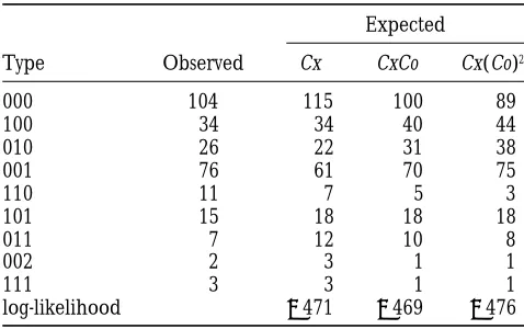
TABLE 12 simulating data sets with the same sample size under the chi-square model, assuming the estimated parameter
Observed and expected number of individuals under
values; (2) estimating model parameters for each
simu-different chi-square models for Neurospora
lated data set; and (3) approximating the standard rors of the parameter estimates using the standard
er-Expected
rors of the estimated parameter values from these
Type Observed Cx CxCo Cx(Co)2
simulated data sets. Using this method, the standard
000 104 115 100 89 errors were estimated to be 1, 1, and 2 cM, respectively.
100 34 34 40 44 Note that the Cx(Co)2model was found to be the best
010 26 22 31 38 model using different sets of Neurospora data (Zhao
001 76 61 70 75 et al. 1995b). The data analyzed in Zhaoet al. (1995b)
110 11 7 5 3
were of unordered type. The difference between the
101 15 18 18 18
estimated best chi-square model could be the result of
011 7 12 10 8
sampling errors or real difference in chiasma
interfer-002 2 3 1 1
111 3 3 1 1 ence among the Neurospora strains used in different
log-likelihood 2471 2469 2476 genetic experiments.
Data fromWhitehouse(1942). Three markers on the
sec-ond chromosome were studied in the order of CEN–Pe –Tu–F. DISCUSSION The observed types are represented by i1i2i3, where i150 or
1 corresponding to FDS or SDS pattern at Pe, i250, 1, or 2 Ordered tetrads studied in this article offer informa-corresponding to parental ditype, tetratype, or nonparental tion both on chromatid interference and on chiasma ditype between Pe and Tu, and i350, 1, or 2 corresponding
interference. In addition, they can be used to map
cen-to parental ditype, tetratype, or nonparental ditype between
tromeres. Although the number of distinguishable
pat-Tu and F.
terns for ordered tetrad is 6n, under RSCA these
distin-guishable types reduce to (6n 1 5 3 2n)/8 distinct
groups. The NCI assumption further reduces the
num-AD–MT can be clearly established. The difference
between the maximized log-likelihood under this order ber of distinct probabilities.
The equality and inequality constraints among or-and the largest maximized log-likelihood under the
other orders is 90. Note that when two markers on dered tetrad probabilities imposed by NCI were derived.
We showed how these general constraints can be used the same chromosome were analyzed, the differences
between the maximized log-likelihood under the best to order markers.
Because it makes use of all the data available, multilo-order and the largest maximized log-likelihood under
other orders were 66 (Table 7) and 58 (Table 8). This cus analysis is advantageous over the analysis in which
only a limited number of markers can be analyzed. For increased difference between the maximized
log-likeli-hoods using three markers, 90 vs. 66 and 58, demonstrates example, for four markers in the order ofA–B–C–D,
using the multilocus approach described above, if mark-the power gained in discriminating different marker
or-ders by simultaneously considering multiple markers. ers A, B, and D are studied in one experiment and
markers A,C, andD are studied in another
experi-Gene-centromere mapping:To illustrate the
applica-tion of the chi-square model to analyzing ordered tetrad ment, data from these two experiments can be analyzed
together to infer the genetic distances among these
data, Neurospora data discussed byWhitehouse(1942,
Table 12) are presented in Table 12, along with the markers. However, if only one or two markers can be
studied in a single analysis, data from the second experi-expected number of observations for each ordered
tet-rad type under the Poisson model, the CxCo model, and ment cannot be used to infer the map distances between
Band other markers.
the Cx(Co)2 model. Three genes were studied: Pe, Tu,
and F on the second chromosome of Neurospora. The We have assumed that genotypes are available at all
markers for all tetrads in our discussion. If genotypes for order of these genes is CEN–Pe–Tu–f. A total of 278
asci were genotyped at these three genes. The largest some markers are missing, the EM algorithm (Dempsteret
al. 1977) can be employed to carry out the likelihood
maximized likelihood was obtained under the CxCo
model in the chi-square model class. Although this indi- analysis efficiently.
Chiasma interference has been observed in many or-cates the presence of chiasma interference, the
differ-ence between the maximum likelihoods under the Pois- ganisms. One difficulty in multilocus analysis has been
to find a good model that both incorporates chiasma son model and the CxCo model is too small to make
any definite conclusions. Under the CxCo model, the interference and permits tractable analysis. Interference
was considered for the analysis of unordered tetrad data map distances were estimated to be 12, 9, and 20 cM
in the three intervals: CEN–Pe, Pe–Tu, and Tu–F. We (RischandLange1983;Zhaoet al. 1995b). Risch and
Lange’s tetrad analysis used the count-location model estimated the standard errors of the parameter