Relationship between DNA polymorphism and fixation time.

(1)

Relationship Between DNA Polymorphism and Fixation Time

Fumio Tajima

National Institute of Genetics, Mishima, 4 1 1 Japan Manuscript received November 13, 1989 Accepted for publication February 26, 1990

ABSTRACT

When there is no recombination among nucleotide sites in DNA sequences, DNA polymorphism and fixation of mutants at nucleotide sites are mutually related. Using the method of gene genealogy, the relationship between the DNA polymorphism and the fixation of mutant nucleotide was quantitatively investigated under the assumption that mutants are selectively neutral, that there is no recombination among nucleotide sites, and that the population is a random mating population with N diploid individuals. The results obtained indicate that the expected number of nucleotide differences between two DNA sequences randomly sampled from the population is 42% less when a mutant at a particular nucleotide site reaches fixation than at a random time, and that heterozygosity is also expected to be less when fixation takes place than at a random time, but the amount of reduction depends on the value of 4Nv in this case, where v is the mutation rate per DNA sequence per generation. The formula for obtaining the expected number of nucleotide differences between the two DNA sequences for a given fixation time is also derived, and indicates that, even when it takes a large number of generations for a mutant to reach fixation, this number is 33% less than at a random time. The computer simulation conducted suggests that the expected number of nucleotide differences between the two DNA sequences at the time when an advantageous mutant becomes fixed is essentially the same as that of neutral mutant if the fixation time is the same. The effect of recombination on the amount of DNA polymorphism was also investigated by using computer simulation.

D

N A

polymorphism and fixation of mutants at nucleotide sites are not independent phenom- ena, but they are mutually related. For example, the fixation of selectively advantageous allele at one locus can reduce the amount of polymorphism at linked locus (KOJIMA and SCHAEFFER 1967; MAYNARD SMITH

and HAIGH 1974; OHTA and KIMURA 1975). Recently

KAPLAN, HUDSON and LANGLEY (1989) have exam-

ined this hitchhiking effect at the

D N A

level, and concluded that in the region of low crossing over the fixation of selectively advantageous mutant at one nucleotide site can substantially reduce the number of segregating or polymorphic nucleotide sites in a sample of

D N A

sequences from that expected under the neutral mutation model.

T h e effect of the fixation of a mutant on the amount

of polymorphism may occur even when the mutant is selectively neutral. WATTERSON (1 982a,b) has shown under the neutral mutation model that fixations tend to occur in clusters rather than behave as a Poisson process. This suggests that there might be some effect of fixation on

D N A

polymorphism even if all the mutants are selectively neutral.

T h e purpose of this paper is to examine quantitatively the relationship between the

D N A

polymorphism and the fixation of a mutant nucleotide.

T h e amount of

D N A

polymorphism can be measured by the average number of (pairwise) nucleotide

Genetics 125: 447-454 (Ju ne , 1990)

differences among a sample of

D N A

sequences or by the number of segregating (or polymorphic) sites in a sample of

D N A

sequences [for their statistical prop- erties under the neutral mutation model, see WAT-

TERSON (1 975) and TAJIMA (1 983)]. In this paper we use the expected number of nucleotide differences between two

D N A

sequences randomly sampled from a population as a measure of the amount of

D N A

polymorphism. This number equals not only the ex- pectation of the average number of nucleotide differences among a sample of

D N A

sequences but also the expected number of segregating sites in a sample of two

D N A

sequences.

T h e fixation time is one of the most important quantities that characterize the fixation. In this paper we study the relationship between the amount of

D N A

polymorphism at the time when a mutant at a particular nucleotide site has fixed and the fixation time for this mutant.

THEORY

Assumptions: Consider a random mating popula-

tion with N diploid individuals, so that there are 2N homologous

D N A

sequences in the population.

As-

(2)

1968, 1983), and that they occur at the rate of v per DNA sequence per generation.

Fixation time: Using the diffusion model, KIMURA

(1 970) has obtained the probability distribution, y ( t ) ,

of the number of generations until a newly arisen mutant becomes fixed in the population, excluding the cases where the mutant is lost from it, which is given by

m

y ( t ) = c ( 2 i

+

I)(-I)+'Xiexp(-Xit), (1)

i= I

where t

>

0 and Xi =

i(i

+

1)/(4N). Let us obtain this probability, using the method of gene genealogy or coalescent process, since this method directly gives the relationship between fixation and polymorphism as will be shown later.

In order to study branch length and branching pattern, we use the Wright-Fisher model with nonoverlapping generations and Moran's model, respectively. This is because branching pattern can be more easily studied by using Moran's model than the Wright-Fisher model. Needless to say, the mixed use of different models may not be desirable. However, some quantities obtained from the Wright-Fisher model are known to be approximately the same as those of Moran's model although certain changes of definitions, e.g., time scaling and the effective population size, are necessary (KINGMAN 1982a,b; WAT-

TERSON 1984). Furthermore, as will be shown later,

computer simulations conducted indicate that this treatment does not cause any serious error.

Let us now consider the genealogical relationship of DNA sequences when the fixation takes place. We assume that at each unit of time one of the 2N DNA sequences is randomly chosen to die, and it is replaced

by a replicate of a randomly chosen sequence from the remaining 2N

-

1 DNA sequences. This model is called MORAN'S (1958) model, though it is slightly different from Moran's original model [see WATTER-

SON (1982a)l. One example of the birth and death

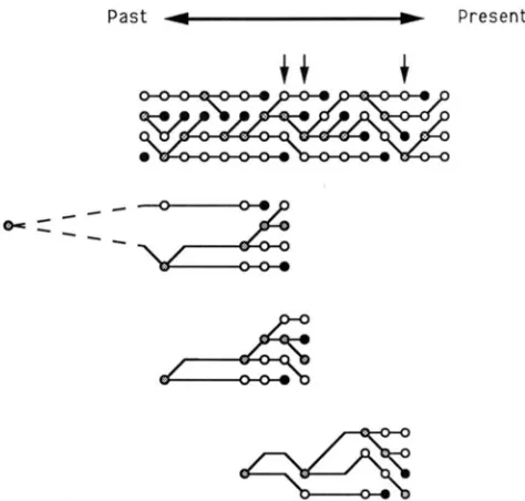
process in Moran's model is shown in Figure 1 where 2N = 4 is assumed. In this example three events of

fixation are possible, as indicated by arrows. This can be explained in terms of gene genealogy. First, 2N DNA sequences from the present population, which are assumed to be mutants, came from 2N

-

1 DNA sequences at the immediately previous time. At this time the remaining one DNA sequence is not the mutant. Then, these 2N

-

1 mutant DNA sequences have the original mutant DNA sequence as common ancestor at some time in the past, and the remaining one nonmutant DNA sequence has an ancestor at this time which is a nonmutant DNA sequence. Figure 1 shows the three genealogical relationships where the fixations can take place in this example. T h e distribution of the genealogical relationship under the con-

P a s t 4

c

Present

+

@-=,

"-

_"

FIGURE 1 .-One example of the birth-death process in Moran's model. The arrows in the top figure indicate the time when fixation can take place. The bottom three figures show the genealogical relationships for the three possible events of fixation.

dition of fixation is different from that without any condition, and this difference is caused by branching pattern, but not by branch length, since there is no restriction on branch length. Because of this, the probability distribution of fixation time can be easily obtained.

Let & ( t ) be the probability that n

+

1 DNA sequences randomly chosen from the population are derived from n DNA sequences for the first time t

generations ago. Using the Wright-Fisher model with nonoverlapping generations, KINCMAN (1 982a), HUD-

SON (1 983) and TAJIMA (1 983) have shown that f n ( t ) is approximately given by

fn(t) = Xnexp(-Xnt), (2)

where the mean and variance are 1/X, and 1/X:, respectively. Then, the probability distribution, y ( t ) ,

of the number of generations until fixation can be obtained from the convolution of h N - l ( t ) , f2~-2(t),

. . .

, f i ( t ) , namely

2N-I

y ( t ) = (2i

+

I ) ( - l ) q

-

X,exp(-Xit). (3)

i= 1 , =I 2N

+

j

'

2 N - j

This equation can be approximately given by

2N-I

y ( t ) = (2i + l)(-I)i+~Xexp[-Xi(t

+ 2)], (4)

i= 1

which is essentially the same as (1).

DNA polymorphism: WATTERSON (1 975) showed

that the expected number, E ( k ) , of nucleotide differences between two DNA sequences randomly sampled from the population is given by

(3)

DNA

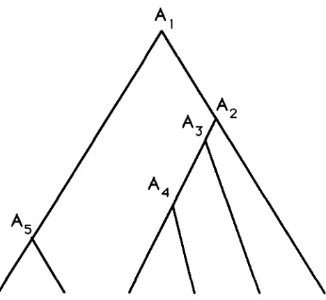
FIGURE 2.-One example of genealogical relationship among six

DNA sequences. A, is the ith oldest ancestor to these six sequences.

where M = 4Nv. This number can easily be obtained

by considering gene genealogies. T h e probability that two randomly chosen

D N A

sequences are derived from their common ancestral sequence for the first time t generations ago isfl(t), which gives the probability distribution of branch length between one of the chosen

D N A

sequences and the common ancestral sequence in terms of the, number of generations, so

that the mean branch length is 1 /X, or 2 N . Since there are two branches between the two sequences randomly chosen from the population, we have

E ( k ) = 2N X 2v = M .

This equation can also be obtained in a different way. Consider the genealogical relationship among

2N

D N A

sequences. When two

D N A

sequences are randomly chosen from these 2N sequences, there are

2N

-

1 possible ancestral sequences. Denote the ith oldest possible ancestral sequence by A;. One example is shown in Figure 2 , where 2N = 6 is assumed. Also

denote by ai the probability that the common ancestral sequence to two sequences chosen at random is Ai.

As

shown in the APPENDIX, this probability is given by

2(2N

+

1)

ai = (i

+

l)(i

+

2)(2N

-

1)'

where 1 S i d 2N

-

1. For example, when 2N = 6,

we have a l = 7/15, a2 = 7/30, a3 = 7/50, a4 = 7/75, and a5 = 1/15. When Ai is the common ancestor, the expected number, E(ki), of nucleotide differences between the two sequences is

This equation can be obtained as follows: First, we

notice from ( 2 ) that v/X, mutations are expected to take place on each sequence while

j

+

1 sequences are derived f r o m j sequences. Considering two sequences, we obtain

(7)

since we can detect all the mutations in the infinite site model. Then, the expected number of nucleotide differences between two

D N A

sequences randomly chosen from the population is given by

2 N - I

E ( k ) = aiE(ki) = M .

i= 1

Thus, we obtain (5).

Using the infinite allele model, KIMURA and CROW

(1964) have shown that the expected homozygosity,

E ( F ) , or the probability that the randomly chosen two

D N A

sequences is identical is given by

1 1 + M ' E ( F ) = ~

This equation can be obtained in the same way as the above, namely, we have

2 N - 1

E ( F ) =

C

aiE(Fi), (9) I= 1

where E(FJ is the expected homozygosity when Ai is the common ancestor to the randomly chosen two sequences. Since the probability distribution of the number of generations between A, and A,+l is given by ( 2 ) , we have

2 N - 1

E(Fa) =

n

bj, (10)

j=;

where bj is given by

In these equations bj is the probability that there is no mutation on the two sequences while

j

+

1 sequences are derived from

j

sequences. Since the expected homozygosity is given by the product of bj's, we obtain (1 0). Substituting (1 0) into (9), we obtain (8).

DNA polymorphism at the time of fixation: Let

us now study

D N A

polymorphism at the time when a mutant at a particular site has fixed. In this case the genealogy of 2N

D N A

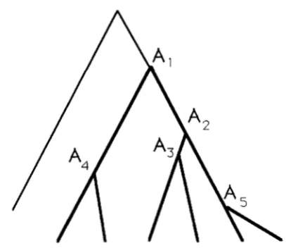
sequences shows unique topol- ogies as mentioned earlier. Figure 3 gives one example where 2N = 6 is assumed.

(4)

Tajima

2 N - 1

FIGURE 3.-One example of genealogical relationship among six

DNA sequences, given that fixation took place. A, is the ith oldest ancestor to these six sequences. Bold lines show the sequences with the mutant nucleotide fixed.

a,, that the common ancestor of the two randomly chosen sequences is Ai is given by (6), as shown earlier. T h e expected number, E(ki

I

fix), of nucleotide differences between the two sequences when A; is their common ancestor is given by

2N- 1

This equation can be obtained by replacing i with i

+

1 in

(7)

since there are

i

+

1 sequences, namely i

mutant sequences and one nonmutant sequence, at the time when Ai occurred. Then, E(k

I

fix) is given by

2 N - 2

E ( k

I

fix) = aiE(ki

I

fix), (1

2)

1= 1

which approximately becomes

E(k

I

fix) =

2 (T

-

3

)

M = 0.5797

...

M . (13)

This formula indicates that, when fixation takes place, the average number of nucleotide differences is expected to be 42% less than at a random time.

Using the infinite allele model, the expected homozygosity, E(F

I

fix), at the time of fixation can be obtained in exactly the same way as the above. Namely, we have

2 N - 2

E(F

I

fix) = u,E(F~

I

fix), (14)

i= 1

where E(Fi

I

fix) is given by

2 N - 1

E(Fi

I

fix) =

n

bJ.

j = t + l

This formula can be simplified as

which is approximately given by

E(F

I

fix) = [ 1

-

exp(-M

+

c1M2

-

c2M3)]/M, (16) where c1 = (47r2

-

39)/6 = 0.07973

...

and c2 = (79

-

8a2)/3 = 0.01438

... .

From this formula we can see that, when fixation takes place, the amount of polymorphism in terms of heterozygosity is also expected to be less than at random times, but the amount of reduction depends on the value of M .

DNA polymorphism for a given fixation time: Let

us now study the expected number, E(k

I

T ) , of nucleotide differences between the two DNA sequences randomly chosen from the population at the time of fixation, given that the fixation time is T . As mentioned earlier, the probability distribution of fixation time can be obtained from the convolution ofJ;(t)'s for all i's, where j ( t ) is given by

(2).

This can be expressed as

where gi(t) can be obtained from the convolution of

f ; ( t ) ' s for all j ' s exceptj = i. T h e conditional expecta- tion, E(ti

I

T ) , of the number of generations between

Ai-1 and Ai, which has the probability distributionj(t),

can be given by

E(ti

I

7')

= G(T)/J(T), (1

7)

where zi(T) is given by

zi(T) = g(t)gi(T

-

t)dt. (18)

y ( T ) can be obtained by using (3) or (4), and z;(T) can

be given by

2 N - 1 2 N - k X,

z:(T) = (2j

+

1) (-ly'+'

n

-

j= 1 k = l 2N

+

k

Xi

-

A,

J#i

-[exp (-hjT)

-

exp(-hiT)]

+

(2i

+

l)(-lyl

2 N - k

k = l 2N

+

k

e n

-

XiT exp (-X,T), (19)

which is approximately given by

2N-1

Zi(T) = (2j

+

l)(-I)j+l

j= 1 hi

-

hj

j#i

-

exp(-hiT)]exp(-2Xj)

+

(2i

+

1)(-1Y+'hiT exp[-hi(T

+ 2)].

(20)

In the same way as the above, the expected number, E(ki

I

T ) , of nucleotide differences between the two 2N

+

1

(5)

DNA Polymorphism and Fixation Time

DNA sequences when their common ancestor is Ai,

given that the fixation time is T , is given by

2N-1

E(ki

I

T ) = 2vE(t,

I

T ) . (2 1 )

j = i + l

Since the probability that Ai is the common ancestor to the randomly chosen two sequences is ai, the expected number, E(k

I

T ) , of nucleotide differences between the two DNA sequences randomly chosen from the population at the time of fixation, given that the fixation time is T , is given by

2N-2

E(k

I

T ) =

C

a B ( k

I

T ) , (22) i= 1

which can be simplified as

2 N - 2

E(k

I

T ) = 2vdiE(ti+l

I

T ) , (23)

i= 1

where di is given by

i(2N

+

1)

di

= (i

+

2)(2N

-

1)'

Although numerical examples will be shown later, here we notice that, as T increases, E(ti

I

T ) approaches

4N

E(ti

I

00) =

(i

-

l)(i

+

2)'

so that from (23) we have

E(k

I

00) = 2(2N

-

2)M 2

3(2N

-

1 ) z

-

3 M = 0.6666

...

M. (25)

This formula indicates that, even when it takes a large number of generations for a mutant to reach fixation, the amount of DNA polymorphism at the time of

fixation, in terms of the number of nucleotide differences between the two DNA sequences randomly chosen from the population or the average number of (pairwise) nucleotide differences among a sample of sequences, is expected to be 33% less than at a random time.

NUMERICAL EXAMPLES AND COMPUTER SIMULATION

In order to check the accuracy of the formulae obtained, computer simulations were conducted. T o save computer time, the telescoping method proposed

by KIMURA and TAKAHATA ( 1 983) was used, which is an improved version of the pseudosampling-variable method (KIMURA 1980).

Neutral mutation: First, we consider the case where a newly arisen mutant is selectively neutral. Let xi be the relative frequency of mutant at generation i. As- sume that there is no mutant at generation 0 and a new mutation takes place at generation 1 , so that x. = 0 and x1 = 1/(2N). Then, we start computer simu-

TABLE 1

Results of computer simulation

~~~ ~~ ~

Average no. of nu- Fixation No. of Average fix- cleotide differences

time cases ation time between two DNAs"

-49 50-99 100-149 150-199 200-249 250-299 300-349 350-399 400-449 450-499 500-549 550-599 600-649 650-699 700-749 750-799 800-849 850-899 900-949 950-999 1000- Total 0 29 89.5

351 131.3 947 177.6

1,226 225.4 1,316 275.0 1,223 324.1 1,013 375.0

828 423.9 662 474.5 512 522.9 424 572.6

327 623.4 227 674.2 1 80 723.1

149 773.8 129 823.1 114 874.6 73 924.2 67 976.8 203 1,196.2

10,000 399.1

0.301 0.374 0.450 0.501 0.547 0.576 0.596 0.622 0.621 0.654 0.651 0.662 0.688 0.680 0.679 0.650 0.690 0.688 0.666 0.639 0.573

This number is measured with 4Nu.

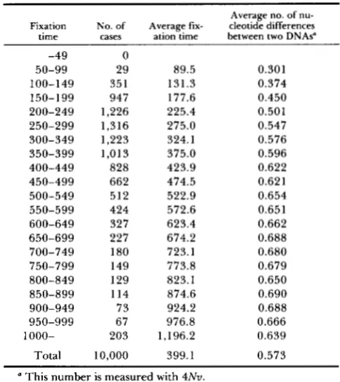
lation followed by the telescoping method and record the frequency of mutant at every generation until the mutant reaches fixation or extinction. In the case of extinction we discard all the records and repeat the simulation from the beginning. In this simulation the population size (N) was assumed to be 100 and we have obtained 10,000 events of fixation.

From a set of data we can easily obtain the fixation time. Since the probability that the two randomly chosen mutant sequences at generation i

+

1 has their common ancestor at generation i is 1/(2Nxi), the expected number of nucleotide differences between the two sequences can be obtained, using

repeatedly until fixation, where E(k1) = 0. T h e result of computer simulation is shown in Table 1 . T h e average fixation time obtained was 399 generations, which is almost the same as 4 N . T h e average of the expected number of nucleotide differences between the two DNA sequences obtained was 0.573M. This indicates that ( 1 3) is a good approximation. Figure 4,

(6)

Tajima

Fixatlon tlme (in generations)

FIGURE 4.-Relationship between the expected number of nu- cleotide differences between the two DNA sequences randomly sampled from the population and the fixation time, where N = 100

was assumed. The line was obtained from (23) with (17), (4) and (20). Closed circles are the results of computer simulation, whose data are shown in Table 1.

line that was obtained by using ( 2 3 ) with (17), ( 4 ) and

( 2 0 ) shows a good agreement with the result of simulation.

Advantageous mutation: So far we consider only

the case of neutral mutation. Here we examine the effect of an advantageous mutant on the expected number of nucleotide differences between the two sequences, using computer simulation. If we denote

by s the selective advantage of mutant over nonmutant, the mean rate of change in xi per generation is approximately given by

h i = S X i ( 1

-

Xi).

Then, computer simulation was conducted under this selection model, where s = 0.005, 0.01, 0 . 0 2 , 0.05,

0.1 and 0 . 2 are used together with s = 0. T h e method of simulation is the same as the above, except the change in frequency of the mutant is affected by

selection. For each value of s, 100 events of fixation were collected, where N = 100 was also assumed.

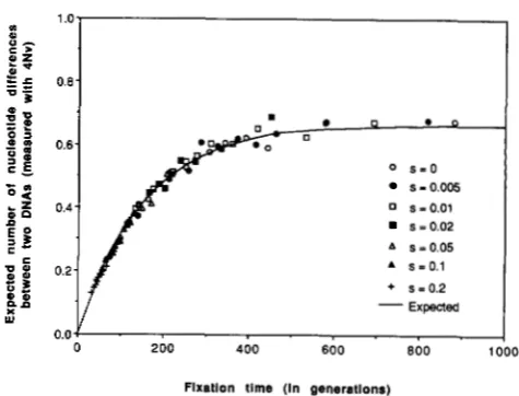
T h e results of simulation are shown in Figure 5 ,

where each point is the sum of ten replicates classified according to the length of fixation time so that there are ten points for each value of s. Interestingly, this figure shows that the expected number of nucleotide differences between the two sequences at the time when an advantageous mutant becomes fixed is essentially the same as that of neutral mutant if the fixation time is the same. It should be noted here that the fixation of an advantageous mutant tends to reduce the amount of

D N A

polymorphism more strongly than that of a neutral mutant since the fixation of an advantageous mutant tends to take place more rapidly than that of a neutral mutation. This conclusion is consistent with that of KAPLAN, HUDSON and LANGLEY

(1 989).

0.6 -

0.4-

A S

-

0.05

A 5 = 0.1

+ s = o . 2

2

0 s s-0.005 s-0.01 = 0.02

- _Expected

0.0

0 200 400 600 800 ₁

Fixation time (in generations)

0

FIGURE 5.-Results of computer simulation conducted under the genic selection model o f advantageous mutation. The line was obtained from (23) with (17), (4) and (20) under the neutral muta- tion model.

Effect of recombination: We have shown that the

amount of

D N A

polymorphism is less when a mutant at a particular nucleotide site becomes fixed, com- pared to random times. This conclusion was obtained under the assumption that there is no recombination in

D N A

sequence. When there is some recombination, the degree of reduction might not be so large as that of no recombination. To know it quantitatively, computer simulation was conducted.

Let r be the recombination rate between the site where a mutant fixes and sites where divergence is being considered, and xi be the relative frequency of the mutant at generation i. Then, RICHARD R. HUD-

SON (personal communication) has shown that the expected number of nucleotide differences between two sequences can be obtained by using

1 R ( l -xi)

2Nxi 2N

R( 1

-

xi) M

+

E ( k ( )

+

-

2N 2N '

Rx, R( 1

-

xi) M

+

E@:)

+

4N

E(V)

+

-

2N ' (27b)

1

2N( 1

-

xi) 2N E(k:)

R x ~ M + - E ( k 0

+

-

2N 2N '

(7)

TABLE 2

Expected number of nucleotide differences between two DNA sequences when a mutant at a linked site is fixed, obtained by computer simulation

Selection coefficient ( 5 )

4Nr 0 0.005 0.01 0.02 0.05 0.1 0.2

0 0.576 0.573 0.552 0.506 0.380 0.266 0.170 0.01 0.579 0.577 0.555 0.508 0.381 0.268 0.170 0.1 0.607 0.604 0.578 0.527 0.394 0.277 0.177 0.2 0.634 0.631 0.602 0.547 0.408 0.287 0.184 0.5 0.700 0.696 0.662 0.599 0.448 0.316 0.204

1 0.773 0.769 0.734 0.667 0.507 0.362 0.237 2 0.855 0.851 0.821 0.760 0.601 0.442 0.298 5 0.941 0.938 0.923 0.886 0.769 0.616 0.450

10 0.977 0.975 0.969 0.95 1 0.887 0.778 0.625

20 0.993 0.992 0.990 0.984 0.959 0.907 0.810

Average fixation time 40 1 389 326 244 138 82 47

N = 100 and 4Nv = 1 were assumed. For each selection coefficient, 5 , 1000 events of fixation were collected.

a

0 1 0 0 200 3 0 0

0 1 0 0 200 300 Tlmo In genorrtlona

b

0 . 4 ! . I . , . , . , I 0 2 0 0 5 0 1 5 0 1 0 0

0 1 0 0 5 0

1 5 0 200

Tlmo In gananilona

1.2

-

0.4

0.2

0.0

0 1 0 2 0 3 0 4 0

Tlmo In ganantlonr

FIGURE 6 , " T h r e e examples of the changes in the frequency of DNA sequence with mutant nucleotide and in the expected number of nucleotide differences between the two DNA sequences randomly chosen from the population which were obtained from the computer simulation where N = 100 was assumed. (a) s = 0 and T = 367; (b) s = 0.02 and T = 220; (c) s = 0.2 and T = 45.

ber of nucleotide differences between two sequences one bearing the mutant and one not, and E(k:) is the expected number of nucleotide differences for two sequences not bearing the mutation. These three equations can be derived from (26) with the same reasoning as equations (1 5 ) of KAPLAN, HUDSON and

LANGLEY (1 989), assuming r

<<

1. Starting from E(k1)

= 0 and E ( k ; ) = E ( k ; ) = 4Nv, we obtain E(ki).

T h e method of simulation is the same as the above, except (27) is used instead of (26). In this simulation N = 100 was also assumed, and 4Nv = 1, s = 0 , 0.005,

0.01, 0.02, 0.05, 0.1 and 0.2, and 4Nr = 0 , 0.01, 0.1, 0.2, 0.5, 1, 2, 5, 10 and 20 were used. For each value of s, 1000 events of fixation were collected. T h e

results are shown in Table 2, which indicates that, as the recombination rate increases, the amount of DNA

polymorphism also increases. In the case of a neutral mutant (s = 0), if 4Nr is larger than 10, the amount of polymorphism at a time of fixation is almost the same as that of a random time. This table also indicates that, when a strongly advantageous (s

>

0.1) mutant is fixed, the amount of polymorphism is substantially smaller than at a random time even if 4Nv is larger than 10. This result is consistent with that of KAPLAN,

HUDSON and LANGLEY (1 989).

DISCUSSION

(8)

expected number of nucleotide differences between the two DNA sequences randomly chosen from the population is M (= ~ N v ) , while the number becomes

0.58M at the time of fixation. This difference might be caused by the large amount of DNA polymorphism on the way to fixation. Figure 6 shows some examples of the relationship between the frequency of mutant and the expected number of nucleotide differences between the two sequences, which were obtained from the computer simulation in the previous section. Fig- ure 6a shows the example in the case of s = 0, where the fixation time was 367 generations. In this example the expected number of nucleotide differences is larger than 4Nv when the frequency of mutant is intermediate. This does not occur in the case of rapid fixation as shown in Figure 6c. At any rate, the

amount of DNA polymorphism changes drastically, depending on the frequency of the mutant. This might be one of the main reasons for a large stochastic variance of the amount of DNA polymorphism.

T h e results of the computer simulation conducted have shown that the formulas (22), (23) and ( 2 5 )

obtained under the assumption of neutral mutation also hold in the case of advantageous mutation. This conclusion, however, might be correct only in the genic selection model or the semi-dominant mutation model. In fact, in the case where the advantageous mutation is recessive or dominant the results of the computer simulation conducted in the same way as the above show that this is not the case (data not shown). At any rate more extensive studies are needed for various types of selection model, including over- dominance selection model.

I thank R. R. HUDSON for showing me equations (27) which improved this paper greatly. I also thank R. R. HUDSON and two anonymous reviewers for their valuable suggestions and comments. Contribution No. 1823 from the National Institute of Genetics, Mishima, 41 1 Japan.

LITERATURE CITED

HUDSON, R. R., 1983 Testing the constant-rate neutral allele model with protein sequence data. Evolution 37: 203-217.

KAPLAN, N. L., R. R. HUDSON and C. H. LANGLEY, 1989 The “hitchhiking effect” revisited. Genetics 123: 887-899.

KIMURA, M., 1968 Evolutionary rate at the molecular level. Na- ture 217: 624-626.

KIMURA, M., 1969 The number of heterozygous nucleotide sites maintained in a finite population due to steady flux of mutations. Genetics 61: 893-903.

KIMURA, M., 1970 The length of time required for a selectively neutral mutant to reach fixation through random frequency drift in a finite population. Genet. Res. 1 5 131-133.

KIMURA, M., 1980 Average time until fixation of a mutant allele in a finite population under continued mutation pressure: Studies by analytical, numerical, and pseudo-sampling methods. Proc. Natl. Acad. Sci. USA 77: 522-526.

K I M U R A , M . , 1983 The Neutral Theory of Molecular Evolution.

Cambridge University Press, Cambridge.

KIMURA, M . , and J. F. CROW, 1964 The number of alleles that can be maintained in a finite population. Genetics 4 9 725- 738.

KIMURA, M . , and N. TAKAHATA, 1983 Selective constraint in protein polymorphism: Study of the effective neutral mutation model by using an improved pseudosampling method. Proc. Natl. Acad. Sci. USA 8 0 1048-1052.

KINGMAN, J. F. C., 1982a On the genealogy of large populations.

J. Appl. Probab. 19A: 27-43.

KINGMAN, J. F. C., 1982b Exchangeability and the evolution of large populations, pp. 97-1 12 in Exchangeability in Probability and Statistics, edited by G. KOCH and F. SPIZZICHINO. North- Holland, Amsterdam.

KOJIMA, K. I., and H. E. SCHAEFFER, 1967 Survival process of linked genes. Evolution 21: 5 18-53 1.

MAYNARD SMITH, J., and J. HAIGH, 1974 The hitch-hiking effect of a favorable gene. Genet. Res. 23: 23-35.

MORAN, P. A. P., 1958 Random processes in genetics. Proc. Camb. Philos. SOC. 54: 60-7 1.

OHTA, T., AND M. KIMURA, 1975 The effect of a selected linked locus on heterozygosity of neutral alleles (the hitch-hiking effect). Genet. Res. 25: 313-325.

TAJIMA, F., 1983 Evolutionary relationship of DNA sequences in finite populations. Genetics 105: 437-460.

WATTERSON, G. A., 1975 On the number of segregating sites in genetic models without recombination. Theor. Popul. Biol. 1 0

WATTERSON, G. A., 1982a Substitution times for mutant nucleo-

WATTERSON, G. A., 1982b Mutant substitutions at linked nucleo-

WATTERSON, G. A., 1984 Lines of descent and the coalescent. 256-276.

tides. J. Appl. Probab. 1 9 A 59-70.

tide sites. Adv. Appl. Probab. 14: 206-224.

Theor. Popul. Biol. 2 6 77-92.

Communicating editor: R. R. HUDSON

APPENDIX

Denote by Ai the ith oldest ancestral DNA sequence to a sample of n sequences as shown in Figure 2 . Also

denote by ai,, the probability that the common ancestor to the two sequences randomly chosen from a sample of n sequences is Ai, where 1 d i d n

-

1. First,

we notice that there are pairwise combinations

and that only one of them creates the latest ancestor

(A5 in Figure 2 ) , so that we have

($

&-I,, = 1/($ =

2

n(n

-

1)’ (AI)

After this combination we now have n

-

1 sequences. If we know a,,,-l, then ai,, can be given by

where 1 d i

c

n

-

2. From these equations we have

2(n

+

1)

(i

+

I)(i

+

2)(n

-

1)’

ai,, = ( A 3 )