An Exact Bidirectional Approach to the Resource Constrained Project Scheduling Problem

(1)

Abstract

KARNOUB, RAZEK E. An Exact Bidirectional Approach to the Resource Con-strained Project Scheduling Problem. (Under the direction of Salah E. Elmaghraby)

The aim of this research is to develop a new approach to the Resource Constrained Project Scheduling Problem. Traditionally, most exact approaches to solve the problem have been either Integer Programming approaches or Branch and Bound (BaB) ones. Of the two, BaB procedures have proven to be the more successful computationally. But, while it is quite intuitive to conceive that the root node of a BaB search tree should be the start activity, it is no less conceivable that it be the terminal activity. Indeed, it is conceivable that the search starts from both ends and concludes somewhere in the middle of the ensuing trees. Unfortunately, BaB as a methodology is not amenable to deriving a termination criterion for such a procedure which guarantees optimality. To a large extent, this research can be seen as an attempt at accomplishing just that.

(2)

future.

(3)

An Exact Bidirectional Approach to the Resource

Constrained Project Scheduling Problem

by

Razek E. Karnoub

A dissertation submitted to the Graduate Faculty of North Carolina State University

in partial fulfillment of the requirements for the degree of

Doctor of Philosophy

Operations Research

Raleigh 2001

Approved by:

–––––––––––––– ––––––––––––––

Dr. Bibhuti B. Bhattacharyya Dr. Carla D. Savage

–––––––––––––– ––––––––––––––

(4)

c

(5)

To my parents,

Maha,

(6)

Biography

This preliminary section, required by the graduate school of this university, is generally filled with a glimpse of the author’s personal pre-dissertation life story. While this maybe quite interesting, a dissertation biography would probably be more informative if its author were to concentrate on the life of his or her dissertation and the major issues that eventually shaped it. Such issues, in all likelihood, must have been central to an author’s life for a significant length of time yet they may not have necessarily found their way into the text itself. They, in fact, would tell the story behind the story and as such could be fairly instructive to other researchers in the samefield; especially future dissertation authors.

With this in mind, here is my biography.

(7)

integer diagonal blocks coupled with linear constraints in terms of continuous variables only. But, as it turned out, a procedure to take advantage of such a structure already existed while my research to develop a new exact methodology for it was inconclusive. Subsequently, I took the suggestion of my advisor to come up with a procedure that sort of calculates several moves ahead to pick the best current move. The result was the ‘look-ahead’ heuristic based on integer programming formulations of the problem.

With that, I put my integer programing attempts on hold and shifted my aim to take advantage of the structure of the problem in a direct way. More precisely, I realized that the problem could be modeled as a shortest path problem between two nodes of a network. The diﬃculty was that the network might be so large that it becomes impractical to generate. To ease this diﬃculty, I thought, one could develop rules to fathom a multitude of nodes generated. Additionally, one could apply a shortest path procedure on the network as it is developed rather than after its generation. This potentially allows the procedure to terminate before many possible nodes are actually generated. Further, one could start from both terminal nodes of the network to work out paths from each that meet somewhere in the middle avoiding, in the process, even more inessential nodes. But more generally, one could introduce uniformly directed cutsets into this network, determine the ‘shortest paths’ between nodes associated with consecutive cutsets and ultimately deduce a shortest path between the network’s terminal nodes through the cutsets. Clearly, this would constitute a decomposition, or a multi-directional, approach to the problem; in contrast to the previous approach, more appropriately characterized as bidirectional.

(8)

‘original and substantive’ enough for a dissertation topic while the bidirectional approach would be its mere special case. My initial goal for this dissertation, then, was to develop the multi-directional approach.

Naturally at that point, numerous details had yet to be hammered out. But I was confident enough they eventually could be that I turned my attention towards a thorough literature review of the problem. All the while hoping, of course, that these ideas were not already developed. Fortunately for me, they indeed were not.

Following the literature review, I set out to develop the remaining details of the bidirectional procedure. In this process, a fundamental revision of one of my original ideas had to be made. Restricting the nodes of a network that could be generated entailed that some paths originating at the two terminal nodes may actually not meet at a common node. Resolving this issue required that two networks, not just one, be distinguished and that a new concept of intersecting paths be introduced; with all the implications regarding the recognition of path intersection and the optimality of a resulting schedule.

(9)

(10)

Acknowledgements

It is a pleasure to express my sincere appreciation to all who have provided me their help and assistance in this eﬀort.

My thanks go to Dr Salah E. Elmaghraby, chairman of my advisory committee, for his numerous comments and suggestions, his advice, his hard work and not the least for his patience. Thanks also to the members of my committee, Drs B.B. Bhattacharyya, Carla D. Savage and H.T. Tran, for valuable discussions and helpful comments.

Thanks are also due to my oﬃce-mates Hao Cheng, S.Ilker Birbil, Shunmin Wang and Burcu Özçam. Their help in some of the finer details of the arduous task of debugging my code has been instrumental.

(11)

List of Tables

3.1 J30 - Time Analysis per Group . . . 224 3.2 J30 - Instances for which the Bidirectional Algorithm Performs Slower than Average225 3.3 J30 - Node Analysis per Group . . . 228 3.4 J30 - Instances for which the Bidirectional Algorithm Requires more Nodes than

(15)

List of Figures

1-1 The interdictive graph - AoN representation . . . 3

1-2 The interdictive graph - AoA representation . . . 4

1-3 Theorem 4: case n = 2 - AoN representation. . . 7

1-4 Theorem 4: case n = 3 - AoN representation . . . 7

1-5 Theorem 4: general case - AoN representation . . . 8

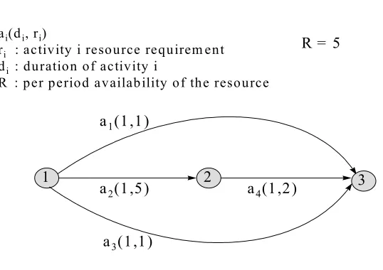
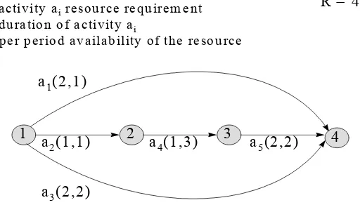
3-1 A project to illustrate the state network concept - AoA representation . . . 105

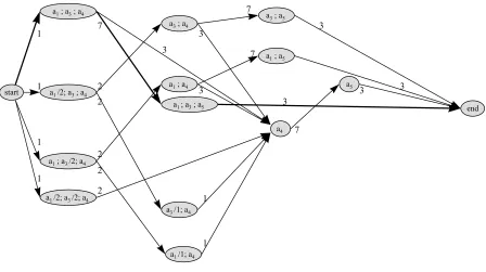
3-2 The state network of the project in Figure 3-1. . . 105

3-3 Counterexample to maximizing resource consumption - single resource, unit du-ration case. . . 108

3-4 Counterexample to maximizing the number of activities started - single resource, unit duration case. . . 108

3-5 Counterexample to generalizing Corollary 10. . . 113

3-6 Graphic depiction of adi-submaximal subset. . . 115

(16)

3-8 The state network of the project instance in Figure 3-1 as reduced by Corollary

15 and Theorem 17. . . 126

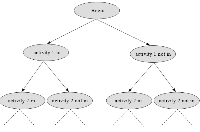
3-9 A decision tree to generate all maximal subsets. . . 142

3-10 The flowcharts for implementing Rules3 and4 in Algorithm 1. . . 146

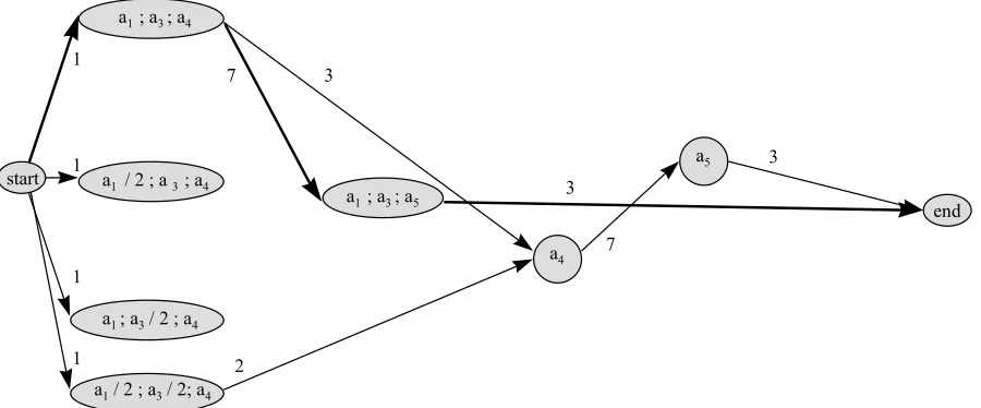
3-11 The reverse reduced state network of the project instance in Figure 3-1. . . 161

3-12 The project instance of Example 26 - AoA representation . . . 178

3-13 The Bidirectional Approach solving the project instance in Figure 3-1. . . 191

(17)

Chapter 1

Introduction, Review and Critique

of Literature

(18)

1.1 Problem De

fi

nition, Graphic Representation and Schedule

Types

TheResource Constrained Project Scheduling Problem, RCPSP for short, is the prob-lem of scheduling a set of activities subject to given precedence relationships among the activities and the availability of the resources required for their completion. In this context, an activity is said to precede another if starting the second requires the completion of thefirst. The objective of the problem is to minimize the project duration under three further assumptions:

• Activity durations are discrete. The time horizon is subdivided into equal periods. Ac-tivities start at the beginning of the periods.

• The activities’ resource consumption levels are given discrete constants over their dura-tions.

• The resource availability limits are constant throughout the duration of the project.

The concept of precedence relationship described above yields naturally the concept of immediate precedence. An activity is said to immediately precede a second if there is no third activity that precedes the second and is preceded by the first. In this case, we also say that the second activity immediately succeeds the first. This concept makes possible a visual representation of a project a lot simpler than it would otherwise be. Indeed, there are two commonly used methods to represent projects that rely on it.

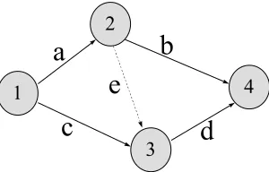
Thefirst method represents an activity by a node and the immediate precedence relationship by an arc. If activity i immediately precedes activity j then the arc points from node i to

(19)

a

b

c

d

Figure 1-1: The interdictive graph - AoN representation

create afictitious activity of zero duration that precedes them. Similarly if there is more than one activity with no successors, we create a fictitious activity of zero duration that succeeds them. These two activities are commonly referred to as thedummy activities. The resulting graphical representation of a project is called the Activity on Node representation, AoN

for short and, for any given project, can be proven to be unique. Figure 1-1 shows the AoN representation of a project of four activitiesa,b,cand d wherea precedesb andd,c precedes d and where the dummy activities are omitted.

(20)

a

b

d

c

1

2

3

4

e

Figure 1-2: The interdictive graph - AoA representation

project is referred to as theActivity on Arcrepresentation,AoAfor short, and is not unique; a project may admit several AoA representations. Figure 1-2 shows the AoA representation of the project in Figure1-1.

The two representations are interchangeable. Given an AoA representation we can easily translate it into an AoN representation. The opposite translation, though, is more diﬃcult due to the non-uniqueness issue which prompts the search for representations with a minimal num-ber of dummy nodes and/or a minimal numnum-ber of dummy activities. Michael, Kamburowski and Stallmann (1993) present a translation that minimizes the use of dummy activities sub-ject to the minimum number of dummy nodes; this problem is NP-Complete but solvable for medium size projects. Given an AoA representation, Bein, Kamburowski and Stallmann (1992) present anO(n2.5₎_{algorithm to minimize the number of its dummy nodes, where} _n_{is the total}

(21)

representation rather because in their context it is the simpler representation.

A schedule of a project is an assignment of starting times to the activities of the project. Note that the earliest possible start times of the activities can be easily computed via a forward pass that ignores the resource constraints. Similarly, given an upper bound on the project duration, the activities’ latest start times can be computed via a backward pass, again ignoring the resource constraints. This yields time intervals during which to schedule the activities to achieve a minimum project makespan. Several types of schedules can be distinguished (cf. Sprecher 1995).

Definition 1 Given a schedule, a local left shift of activity i is a feasible time reduction of the starting time of i, while keeping the starting times of all other activities the same, that can

be accomplished in steps of one time unit decrements. A global left shift of i is a feasible

time reduction of the starting time of i, also while keeping all the other start times the same,

but that cannot result from a local shift of i.

Definition 2 A feasible schedule is said to be semi-activeif no local left shift is possible. A

feasible schedule is said to beactive if no global left shift is possible.

Definition 3 A schedule is said to be non-delay if there is no time period t for which an activity is precedence and resource eligible to be started yet is delayed. A delay schedule is, of

course, one that does allow delaying an activity beyond time t even though it may be eligible to

start at t.

Remark 1 It follows from the definitions that a non-delay schedule is active and that an active

(22)

optimal solution to the RCPSP is active. Hence, searching the active schedules of an RCPSP for

an optimal solution might be more eﬃcient than searching the set of semi-active schedules which

itself might be more eﬃcient than searching the whole set of feasible solutions. Unfortunately,

the set of non-delay schedules might not contain an optimal solution. Worse still, the optimal

non-delay solution can be a very poor approximation of the optimal delay one.

Theorem 4 : For RCPSP, the ratio of the optimal non-delay schedule to its optimal delay one

can be arbitrarily large.

Proof. To prove this assertion, we will show that for any integern_≥2,there exists an RCPSP instance whose ratio of optimal non-delay solution to optimal delay one can be arbitrarily close ton.

Forn= 2consider the RCPSP instance in Figure 1.3; in its AoN representation. By inspection, the optimal non-delay schedule is: 2, 1 and a2, 0, a1, end, of duration max(ε,θ) +ε+θ. In

the same way, the optimal delay schedule is: 2, 1, 0, a1 and a2, end, of durationε+ε+θ. The

ratio of non-delay to delay durations is max(₂ε_ε,₊θ)+_θ ε+θ _→2as ε_→0.

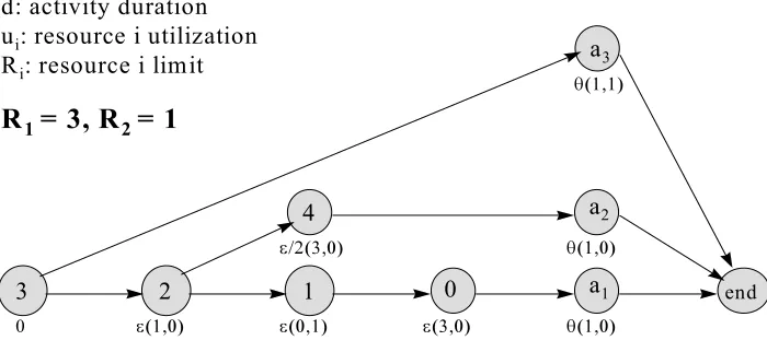
Forn= 3, this instance can be generalized but requires two resources. The generalization is in Figure 1.4. Again by inspection, assuming thatε<θ, the optimal non-delay schedule is: 3, 2 and a3, 1 and (4 and a2), 0, a1, end, of durationθ+ (ε₂+θ) +ε+θ= 3θ+3₂ε. The optimal

delay schedule is: 3, 2, 1 and 4, 0, a1 and a2 and a3, end, of durationε+ε+ε+θ=θ+ 3ε.

The ratio of non-delay to delay durations is 3θ+ 3 2ε

θ+3ε →3 asε→0.

(23)

2 1 0 _a₁ a2

end

0 e(1) e(2) q(1)

q(2)

d(u)

d: activity duration u: resource utilization R: resource limit

R = 3

Figure 1-3: Theorem 4: case n = 2 - AoN representation.

3 2 1 0 a1

a2 a3

end

4

0 e(1,0) e(0,1) e(3,0)

e/2(3,0)

q(1,0) q(1,0) q(1,1)

d(u1,u2)

d: activity duration u_i: resource i utilization R_i: resource i limit

R

₁

= 3, R

₂

= 1

(24)

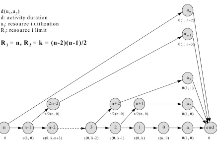
n

2n-2

n-2

n-1 3 2 1 0 a₁ end

n+1

n+2 a₂

a_n-1

a3 a_n

0 _{e(1, 0)} _e(0,k-n₊₃₎ _e(0,k-₂₎ _e(0,k-₁₎ _e(0,k₎ _e(n_,0₎ _{q(1, 0)} 0

q(1, n-2)

q(1, n-3)

q(1, 1)

q(1, 0) e/2(n, 0) _e/2(n, 0) _e/2(n, 0)

d(u1,u2)

d: activity duration

ui: resource i utilization

Ri: resource i lim it

R

₁

= n, R

₂

= k = (n-2)(n-1)/2

(25)

(ε₂ +θ) +ε+θ=nε₂ +nθ.

The optimal delay schedule is n, n-1, n-2 and 2n-2,_{· · ·}, 2 and n+2, 1 and n+1, 0, a1 and a2

and _{· · ·} and an, end, of durationε+ε+· · ·ε+θ=nε+θ. The ratio of optimal non-delay to

optimal delay durations is n

ε

2+nθ

nε+θ →nasε→0.

Remark 2 It may seem that by letting ε _→ 0 in the previous theorem, we have violated the

first assumption made about the durations of activities being discrete. This objection, however,

is easy to deal with. For one, we could have replaced ε with 1_k, where k is a positive integer

and let k _{→ ∞} instead. Even better, we could have fixed ε at 1 and let θ _{→ ∞}. The ratios

of optimal non-delay to optimal delay durations would still be the same in the limit. What is

important is that θbecomes a lot larger than ε.

More than being merely a counter-intuitive mathematical curiosity, this theorem is impor-tant for one approach to RCPSP that it unequivocally rules out. Suppose the theorem is false,

i.e., there is an upper boundM to the ratios of optimal non-delay to optimal delay solutions

of RCPSP instances. It is not too hard to see that the non-delay optimal schedule to RCPSP is a lot easier to obtain than the delay one. Let d∗_n be the optimal non-delay duration of an instance andd∗ _{be its optimal delay one. Suppose we have secured}_d∗

n and a heuristic solution to the delay case of duration h. Then d∗_n/d∗ _≤ M i.e., d∗_n/h_·h/d∗ _≤ M. This says that

(26)

sequence of instances in the theorem shows that those bounds would have to tend to infinity as the number of activities tends to infinity.

1.2 Special Cases and NP-Completeness

Several special cases of RCPSP can be identified. The simplest is the case where resources are in such abundance that they do not constitute any limitation on processing the activities. Here, the forward pass mentioned previously yields a minimum project duration. An optimal feasible schedule is a schedule whose starting times lie in the time intervals derived by the forward and backward passes where the minimum project duration is seen as the project duration estimate of the backward pass. This case is called theCPMmodel.

The opposite of the resource abundance case is the case when the resource limits are one for each resource. A special case of this extreme case is theJob Shop Problem (JSP). It is the problem of schedulingn jobs onm machines. Here the resources are the machines, one of each type, and each job may not need to be processed on each machine but the sequence in which it has to be processed on the machines is given. Except for precedences in the sequences given, no other precedences are imposed. As in the case of RCPSP, the objective is to minimize the makespan. Note that JSP itself is a generalization of the Flowshop Problem(FP). This, in turn, is the problem of scheduling n jobs on a sequence ofm machines. Each job has to go on the m machines in the same sequence. Now, it is well known that FP, for m_≥3, is strongly NP-complete (cf. Pinedo 1995 p. 101)1 _{so JSP must be strongly NP-complete too and therefore}

so must RCPSP. 1

(27)

We remark that this derivation of the strong NP-completeness of RCPSP is not exactly what usually is reported in the literature; for example in Alvarez-Valdes and Tamarit (1989) and Koloisch and Hartmann (1999) to name a couple. More commonly, the derivation is attributed to a result by Blazewiczet al (1983) concerning the strong NP-completeness of JSP with two machines, a single resource, single unit availability and single unit consumptions. We note that neither JSP nor FP in our derivation require resource factors to be incorporated.

1.3 Extensions and Classi

fi

cation

A close look at the defining elements of RCPSP reveals numerous possible ways of extending it. Practical experience necessitated research into most of them. These defining elements are, of course, the activities, the resources, the precedence relationships and the objective. Modifying any of their attributes gives rise to a new problem. This section is devoted to presenting those new problems but we also note that one can extend RCPSP by considering several RCPSP’s simultaneously. The common link between the diﬀerent problems would be a set of shared resources. This problem is called the Multi-Project Scheduling Problem. The obvious way to solve it is to look at it as a single RCPSP. But this may not be the most eﬃcient way. For an early reference to this problem the reader is referred to Kurtulus and Davis (1982).

1.3.1 Activities

(28)

1984, 1985). Another way of modifying activity durations is to allow them to vary in accordance with the amount and/or type of resources spent on them. In this model, a finite number of ways to complete each activity is proposed. Each way comes with its own resource requirements. This problem is called theMulti-Mode RCPSP. Such a model would have applications in the construction industry, for example, where intensive manual labor can be replaced with machine work for substantial savings in time, albeit at a premium cost. For recent a review of exact methods to this problem, the reader is referred to the paper by Hartmann and Drexl (1998). A special case of this problem is theDiscrete Time Resource Trade-oﬀ Problem, DTRTP, which assumes a single resource. A generalization of it is the case where the set of activities is partitioned into subsets. The choice of a mode for one activity forces the same choice on all the activities of the subset to which it belongs. This problem is called the Mode Identity Resource Constrained Project Scheduling Problem, MIRCPSP (Drexl et al 1999).

Now, in certain situations, such as large software development projects, for example, activ-ities can be interrupted during their processing and restarted later with little or no cost. A schedule that permits such action is called a preemptive schedule. The corresponding prob-lem is calledPreemptive-Resume RCPSP. The problem where the preemption cost is not negligible is also of interest, it is called Preemptive-Restart RCPSP. We will have a closer look at Preemptive-Resume RCPSP later. It is also conceivable to impose release dates or due dates, or both, on the activities. In the latter case, the activity is said to possess a time window. Situations also exist where the activities have specific times, calledtime schedule, at which they can start. Note that time windows can be incorporated within the context of Generalized Precedence Relationships which are discussed later in this section.

(29)

RCPSP. A state preserving activity is one that has its start time determined by the activities preceding it and its finish time determined by the ones succeeding it. This might be useful to modeling limited buﬀer space in between two workstations that could lead to blocking. Re-portedly (Klein 2000 p.101), some scheduling software incorporate this concept yet no scientific research has been published to treat it.

1.3.2 Resources

(30)

Examples are the papers by Weglarz (Slowinski and Weglarz 1989) and the paper by Icmeli and Rom (1996).

Another important attribute of resources could be their time dependence. A major cause of this is the temporary unavailability of resources due to sharing them among diﬀerent projects. But there are others such as the scheduled maintenance of machines which results in their temporary unavailability. Time dependent resource availabilities are incorporated within the context of Generalized Precedence Relationships.

1.3.3 Precedence Relationships

The third defining element of RCPSP is the precedence structure. In this model, “activity i precedes activity j” says that i has to be completely finished before j can start. Although this may be the appropriate relationship to model in many situations, it is not suitable for others. For example, activity j may be eligible to start after the start ofi by a given time lag, possibly beforei finishes. This relationship betweeni and j is referred to as a start-to-start

relationship, SS for short. It could also be that j needs to be finished a given time lag after the start ofi. This relationship is calledstart-to-finish, SF. In the same way, we can define

(31)

1.3.4 The Objective Function

Last but not least, the fourth defining element of RCPSP is the objective function. The classic objective has been the minimization of the project duration, ormakespan, denoted byCmax. But this objective can be modified in many ways; each leading to a new perspective on the schedule sought. One way to modify the objective, borrowed from Scheduling Theory, is to impose due dates on the activities. One objective that could be considered, then, is the maxi-mum lateness, Lmax,which calls for minimizing the maximum due date violation. A second

objective is minimizing the tardinessobjective,P j

Tj, whereTj = max(Cj−dj,0), with dj as

the due date of activityj andCjis its completion time. Eﬀectively, it minimizes the average job

tardiness of the feasible schedules. Naturally this can be extended to theweighted tardiness

objective, P_jwjTj, where the w’s are positive weights. A third and fourth objectives, in this

context, could very well be thetotal completion time, P_jCj, which minimizes the average

activity completion time, or theweighted completion time,P_jwjCj.

Another objective modification consists of imposing a deadline on completing the project under which the problem may be infeasible due to lack of resources. To complete the project, additional resources would need to be enlisted in certain time periods at additional costs, of course. The question becomes how to meet the project deadline in minimal cost. This is known as theTime Constrained Project Scheduling Problem, TCPSP. Kolisch (1995) discusses a heuristic to solve it.

(32)

payment is the same irrespective of when it is made, then it is in the interest of the contractor to realize it as soon as possible, so as not to loose some of it to inflation, for example. Additionally, the contractor may want to fund other activities of the project or even redirect the payments towards other projects. Ifr is the inflation rate andpj is the payment for completing activity

j, then j is worth pj.(1−r)Cj upon completion.. It is natural for the contractor, then, to seek

the maximization of P

j

pj.(1−r)Cj subject to the precedence and resource constraints2. This

problem is called the Resource Constrained Net Present Value Problem, RCNPV. It has its own variations and extensions; such as to include generalized precedence relations. For a recent paper on this topic the reader is referred to De Reyck and Herroelen (1998).

Still other objectives than Cmax are the resource leveling objective and the resource invest-ment one. In the Resource Levelling Problem, RLP, the aim is to limit the fluctuations in the resources usage in the hope of reducing the costs associated with thefluctuations. The idea is to obtain the minimum project duration and then possibly reshuﬄe the activities within the minimum project duration to level the resources usage. Bandelloni et al (1994) deal with this problem. The Resource Investment Problem, on the other hand, is the problem of determining the resource requirements of a project given the project duration. It arises in the definition phase of the project rather than in the planning phase. Per period-unit costs are as-sociated with the resources,cr,and an estimate of the makespan is determined. The objective is to minimize the total costP_rcrar wherear denotes the per period availability of resourcer. Demeulemeester (1995) studies this problem.

A radically diﬀerent approach to project scheduling has been studied by Icmeli and Rom (1998). The authors conducted a survey of project managers nationwide and across diﬀerent

2

(33)

industries. The objective of the survey was to determine the most important project character-istics that managers focus on. The result of the survey was that quality was, by far, the most sought after objective. Quality, they state, is manifested when the amount of rework that goes into activities is kept to a minimum. To deal with this issue the authors define a significantly diﬀerent model from RCPSP or its variants mentioned above. The model turns out to be a lot easier to solve than RCPSP (Icmeli and Rom 1997).

Note that all the objectives mentioned so far have been single criterion objectives, at least on the surface. It is conceivable that in some situation one may want to explicitly consider two or more of these objectives either by combining them into one global objective or by approaching them in sequence as in the Goal Programming approach. We also note that one can combine characteristics of the extensions mentioned so far to come up with more variations and extensions. For example, suppose a project requires a single resource and that the activities are multi-modal; the more resource allocated to an activity the shorter its duration and the higher its cost. Assume also that the resource is non-renewable. One may be interested, in this case, in scheduling the activities to minimize the project duration or minimize the project cost or even generate the time/cost trade-oﬀcurve. This problem is called theDiscrete Time Cost Trade-oﬀ Problem, DTCTP, and has been extensively studied since the early days of Project Management. For a treatment of this problem, the reader is referred to Elmaghraby (1977, Chapter 2).

1.3.5 Classi

fi

cation Schemes

(34)

precisely describes any RCPSP variant. It is important that this notation scheme be compatible with the notation scheme that has been adopted for machine scheduling because many problems of the latter are special cases of RCPSP variants. Two such schema have recently been proposed by Herroelenet al . (1999) and Bruckeret al . (1999). A problem description, in both schemes, consists of three fields. The first field is reserved to describe the resource environment, the secondfield describes the activity characteristics, which for both teams includes the precedence structure, and the last field states the objective function being considered. But whereas the Herroelen et al scheme tries to emulate the notation scheme in Scheduling Theory, it is not compatible with that scheme. Additionally, it is elaborate enough so that one would often have to consult the definitions of its parameters to decipher their meanings. The scheme by Brucker et al, on the other hand, is more compatible with that of Scheduling Theory and allows the

practitioner to be less dependent on frequent consultations of the definitions. According to this latter scheme RCPSP is P S_|prec_|Cmax , where ‘PS’ stands for Project Scheduling and

‘prec’ stands for the existence of precedence relationships. It remains to be seen which notation scheme will be adopted by the project scheduling community, if at all.

1.4 Existing Methodologies

(35)

hardware technology, they are bound to eventually change with the advent of new methods and hardware. We shall see in this section that with the current state of aﬀairs, many instances with30activities have been solved by a variety of exact methods and that many instances with 60 activities are so far intractable.

For cases where an instance size is clearly too large for current exact methods, heuristic approaches are the only way to reach a feasible solution. No bound on the quality of the solution can be given, however, as reportedly “no polynomial time approximation algorithm with a performance guarantee less than nε _{” can be given unless} _P ₌ _{N P} _(Möhring _{et al}

1999)3. Herenrepresents the size of an instance andε>0is an arbitrary error parameter. To gauge the quality of a particular heuristic solution, though, lower bounds on the optimal value of an instance furnish what perhaps is the only available test. If a lower bound is judged close enough to a heuristic solution then that solution may rightly be deemed acceptable. Else, if the diﬀerence is seen inadmissible then a better lower bound needs to be obtained and/or the heuristic solution is poor.

In this section we start with a review of some lower bounds. We then move to a review and critique of what presently are, or until quite recently were, viewed as promising exact methods. We end the section with a discussion of heuristics proposed for the problem.

1.4.1 Lower Bounds

We have already mentioned one significant reason for studying lower bound methods. Another important one is their use within the most common exact methods for solving RCPSP: Branch 3_Möhring_{et al} _{reach this conclusion by noting that the same applies to the Node Coloring Problem which,}

(36)

and Bound methods. In such methods, a comparison of the lower bound at a node of the search tree with the current or, sometimes, local upper bound on the optimal solution is needed to decide whether to fathom the corresponding node or not. Additionally for many depth first search methods, the lower bounds at the nodes are also used to select the node from which the search is to proceed from. Namely, the node with the lowest lower bound amongst the descendents of the current one.

(37)

what we think are the more important bounds in the literature; in terms of either eﬀectiveness, widespread use within leading exact methods or just simplicity. Some of these will be more elaborated on with their corresponding exact method in the following subsection.

The CPM Bound

This is one of the simplest lower bounds for RCPSP, both conceptually and computationally. It consists of ignoring the resource limitations and applying the previously mentioned forward pass to obtain the early finish time for the project. This constitutes a lower bound on the optimal project duration. It is not a terribly eﬀective bound but it is computationally cheap. It was used within a revised version of what was perceived as the foremost RCPSP exact procedure of its time, the Demeulemeester and Herroelen procedure of 1992 (cf. Demeulemeester and Herroelen 1997).

A Capacity Bound

This is another simple bound derived by considering, for each resource, the cumulative resource requirement of the project’s activities versus the per period availability of the resource. The lower bound is the maximum of the corresponding ratios over the diﬀerent resources. We are not aware of any competitive exact method that uses this bound. But it could, as we shall shortly see, be part of a more involved lower bound strategy, namely destructive improvement.

A Critical Sequence Lower Bound

(38)

of it was later developed for the same procedure but both were eventually dropped in favor of the simpler and, for that procedure, provenly more eﬀective CPM bound (Demeulemeester and Herroelen 1997). We expand on it in our review of their approach.

A Truncated LP Relaxation Based Bound

This is a bound based on the relaxed integer programming formulation of RCPSP in Mingozzi

et al (1998). In this formulation, all constraint sets but one are eliminated and the remaining

one transformed into an inequality set. The resulting linear program can be generated and solved for projects with up to 30 activities (Brucker et al 1998). For larger size projects, with 60 or 90 activities, its columns become too numerous to generate. But Mingozzi and his collaborators did not report solving it directly for such size problems. Instead, they turned to its dual and came up with the next bound we review, the weighted node packing bound. Brucker and his collaborators (Bruckeret al 1998), on the other hand, made several attempts at a direct solution before they found one they were convinced was the best to use with their procedure (Brucker and Knust 1999). This happened to be a hybrid of column generation and the destructive improvement strategy which we will discuss shortly. Mathematically, it is one of the more sophisticated bounds that we encountered. It is also the best in terms of deviation from the optimum. Not too surprisingly though, its computational burden is one of the largest as well.

A Weighted Node Packing Bound

(39)

and going through a sequence of truncated, relaxed, dualized and integerized versions of it. We cover this approach in our review of the procedure but note that it can also be derived more simply by the following argument in Klein (2000).

Basically, if two activities cannot run concurrently due to precedence relationships or re-source requirements then they must be scheduled sequentially. Hence, a subset of the activities that pairwise cannot be concurrent must have its total of the activities’ durations as a lower bound on the optimal duration of the project. Constructing a graph to model the situation where each vertex matches an activity, each vertex weight matches the duration of its corre-sponding activity and each edge corresponds to the feasibility that the activities matching its adjacent vertices be concurrent, one realizes that the goal must be to find the independent subset of the graph with maximum total weight4_{. This is exactly the Weighted Node Packing}

Problem that Mingozzi and his colleagues arrived at.

Since the problem is NP-Complete, the authors solve it heuristically to obtain a relatively good and not too expensive bound. Demeulemeester and Herroelen (1997) used the same model but a diﬀerent heuristic as the lower bound of their updated procedure. Sprecher used still a third heuristic for his (Sprecher 2000). Furthermore, Klein and Scholl have developed one extended and another generalized versions of this same bound that reportedly are more computationally expensive but tighter (Klein 2000).

4_{A set of vertices of a graph is said to be independent if no two vertices in the set are adjacent (}_i.e. _connected

(40)

The Destructive Improvement Strategy

This is a general strategy that can be adapted to deduce a lower bound, or even an optimal solution, for many types of problems not just RCPSP. The basic idea is as follows. Starting with an arbitrary lower bound LB, examine the bound extensively to detect whether it might be infeasible. If infeasible, the bound can be increased by at least one and the process restarted. Otherwise if infeasibility cannot be proven, the lower bound has to be accepted. Needless to say, the eﬀectiveness of this strategy strongly relies on the eﬀectiveness of the infeasibility test, or tests, employed.

Klein and Scholl’s adaptation of this strategy to RCPSP (Klein 2000) involves a two-phase infeasibility test. The first phase consists of applying so called reduction techniques with the aim of deducing sharp time windows for the activities of the project. It is quite possible that while deducing these time windows, an infeasibility of the lower bound is detected. But if not, the test moves to its second phase. Here, the time windows are used in the application of several simple lower bound techniques, such as any or all of the previously mentioned ones albeit possibly with some modification. If a lower bound is detected that is larger than the latest one used in the reduction techniques then we know that this latter one, i.e.,the bound used in the reduction techniques, is infeasible and so must be increased to the newly deduced one5_{. If not then the same simple lower bound techniques are applied to judiciously chosen}

time intervals in a further eﬀort to detect infeasibility6.

To illustrate what those reduction techniques are about, we present one based on the 5_{Klein doesn’t quite make this conclusion but we think this step is in the spirit of the same strategy.} 6

(41)

notion ofcore timeof an activity. Given an estimate of a project’s duration, this is the interval of latest start/earliestfinish times of the activity. This interval is empty when the earliestfinish time is less than the latest start time but otherwise its length never exceeds the duration of the activity7. This says that an activity is active in its core time, if one exists. Now, with the existing core times, the resource requirements are checked against their limits. If the limits are violated then the lower bound is infeasible and so has to be increased. If they are not, each activity is tested for scheduling within its time window taking into account the resource requirements of the other activities within their core times only. If, in this case, it so happens that an activity cannot be scheduled within its time window then the lower bound is infeasible. But if it happens that an activity can be started at only one possible time then this starting time is fixed and the time windows of the other activities are adjusted accordingly. This may result in new time cores in which case the process is repeated. If, on the other hand, one of the activities cannot be scheduled within its time window then the lower bound is again infeasible and has to be increased.

Now, the Klein and Scholl’s destructive improvement lower bound for RCPSP in its full version includes two more reduction techniques and eight simple lower bounding techniques, four of which are all the previously mentioned ones except for the truncated LP relaxation bound. Clearly then, we have only covered its essence here. Computational results by the authors show that the full version is one of the best lower bounds available for RCPSP, in terms of deviation from the optimum, though it is not as strong as the Brucker and Knust hybrid bound and requires the longer running time of the two on the J60 instances (Klein 2000)8. 7_{If the core time of an activity has length larger than its duration then the earliest start of the activity is}

larger than its latest start which is absurde.

(42)

More importantly, computational experiments also show that ‘lite’ versions of the full one run a lot faster and for only a small reduction in bound quality. Evidently then, the choice of which version of this bound to use with which procedure can only be procedure dependent.

A Lagrangian Relaxation Bound

This is a bound by Möhring et al (1999) based on an integer programming formulation of the similar problem with temporal constraints instead of simple precedences. Ifiandjare two of a project’s activities, a temporal constraint betweeniand j takes the form: Sj ≥Si+dij, where

Sk is the start time of an activityk and dij is a time lag that could be negative. Note that if

dij is the duration of activityithen the temporal constraint reduces to the regular precedence relationship. Consider a project of n+ 2 activities including the two dummy ones. LetT be an estimate of the project duration. For all j = 0, . . . , n+ 1 and t = 0, . . . , T, let xjt = 1 if activityj starts at time tand xjt = 0otherwise. LetH be the set of pairs of activities iandj with temporal constrains among them and let dij denote the corresponding time lags. Letrjk be the requirement of activityjfrom resourcekand letRk be the availability of that resource. Finally, letpj be the duration of activityj. The problem can be formulated as:

(P) : M inX

t

txn+1,t

s.t. X

t

xjt = 1,∀ j,

T

X

s=t

xis+

t+_Xdij−1

s=0

xjs ≤ 1,∀(i, j)∈H and ∀t,

X j rjk   t X

s=t−pj+1

xjs 

 _≤ Rk,∀k, t,

(43)

The first set of constraints insures that an activity is started only once. The second insures that if(i, j)_∈H and istarts on or after timetthen activityj cannot start by time t+dij−1, i.e., it must start on or after time t+dij. Since this is particularly true if activity istarts at time t, the time lag between i and j is preserved. The third set of constraints clearly insures that the resource limits are preserved. We note here that the restriction of this formulation to RCPSP, i.e., the case where dij = pi for all (i, j) ∈H, has much in common with one of the first mathematical formulations of RCPSP; namely that of Pritskeret al (1969). The diﬀerence between the two is the second set of constraints which in the formulation here has T + 1 as many constraints and so is stronger when relaxations of the integer programs are considered.

To obtain their lower bound, Möhring and his collaborators propose a Lagrangian relaxation of the above model in which the third set of constraints is dualized. As with any Lagrangian relaxation procedure, ifλ_≥0is the multiplier used to dualize the constraints then the minimum value of the Lagrangian, for fixed λ, is a lower bound on the optimal objective value of the original problem. Therefore, to obtain the best lower bound on that optimal value, the aim should be to find the λ _≥ 0 that maximizes the lower bound. Usually, and this is what the researchers have done, the maximization is done using subgradient optimization which utilizes the optimalx∗(λ) from the Lagrangian minimization step. Now, other researchers have previously used this same approach; namely Christofedes, Alvarez-Valdez and Tamarit (1987)9. But whereas Christofedes and his collaborators have used a Branch and Bound procedure to obtain the optimal x∗(λ), Möhring and his collaborators remark that it has subsequently been shown that LP relaxation of the Lagrangian has an integral solution anyway and, in a further push, transform it into a Minimum-Cut problem for an even faster solution.

9

(44)

The resulting lower bound has been compared to the Mingozzi et al node packing bound and to the Brucker and Knust column generation/destructive improvement bound on the J60, J90 and J120 data sets which we discuss in a latter section. The authors report that their lower bound is tighter than thefirst but that it is not as sharp as the second, though it is much faster.

1.4.2 Exact Methods

Indubitably, the most compelling and most obvious reason for developing exact methods for any problem is to obtain proven optimal solutions for it, to be certain that once such a solution is secured no other possible solution out there can be any better. Naturally, when several exact methods for a problem are available, the question of which of those is the more efficient is swiftly raised. Efficiency, here, could be in terms of computer execution speed and/or required memory space but, regardless, for NP-Complete problems it ultimately translates into the largest size for which an instance is solvable on a given computer with a given configuration and in a given amount of time. Consequently, a second reason to develop an exact method for an NP-Complete problem is to attempt to expand the size of what generally is recognized as a solvable instance in reasonable time. Still, a third important reason is to provide a direct means to assess the quality of lower bounds and heuristics on small size instances in an effort to gauge their quality on larger size instances where exact methods are simply impractical.

(45)

the solutions sought has prompted the research into techniques of the second class (Patterson 1984). Within the class of enumerative methods, several approaches could be distinguished among which are Dynamic Programming, Implicit Enumeration, Bounded Enumeration and Branch and Bound. Among these, Branch and Bound methods were eventually recognized as the most successful. But as we shall see, success here is only relative as the size of instances that can generally be expected to be solved within reasonable time remains rather small.

This subsection is devoted to the review and critique of what we came across in the literature as the more successful exact procedures. They happen to be all of the Branch and Bound variety. Each of these is based on a completely diﬀerent perspective of how a solution to the problem should be derived. Thefirst family we examine, the DH family, has until recently been recognized as the family of the most eﬃcient exact methods for RCPSP. The second procedure we shall be interested in, BBLB3, outperforms thefirst on certain types of problems but more importantly has generated the previously mentioned popular LB3 bound. The third, BKST, has prompted the creation of a heuristic and the best lower bound available for the problem. The fourth, GSA, employs an extensive array of dominance rules. And last but not least, the last two procedures, Progress and Scatter, are not only very competitive computationally but also implement new concepts for Branch and Bound that could very well be employed for other types of problems.

We have intentionally left out, from this review, methods that eventhough were interesting from a theoretical point of view, were not competitive computationally. Noteworthy among these are the bounded enumeration procedure of Davis and Heidorn (1971), the implicit enu-meration procedure of Talbot and Patterson (1978), the branch and bound procedure of Stinson

(46)

procedure of Simpson and Patterson (1993) and the recent fractional cutting plane algorithm of Sankaranet al (1999). Two interesting studies, from a mathematical point of view, that we have also left out are one by Möhring and Radermacher (1989) and another by Alvarez-Valdés and Tamarit (1993). Thefirst discusses, among other concepts, the issue of project decomposition. The second discusses the facets of the feasible polyhedron of a disjunctive integer programming formulation of the problem and introduces cutting planes to help in its solution.

The DH Procedures

These are three RCPSP procedures that Demeulemeester and Herroelen have introduced start-ing in 1992. Each successive procedure is based on its predecessor and is meant to be a significant improvement over it. All are branch-and-bound (BaB) based. In the following, we describe the first, which the authors refer to asDH, and then point out the changes that make up the second and third improvements. Thefirst procedure was later adapted for the preemptive RCPSP (the resume variant). We briefly describe that one last in this subsection.

The nodes of the BaB tree of the DH procedure correspond to partial schedulesP Sm at timesm= 1,2,_{· · ·}where temporaryfinish times are assigned to a subset of the activities of the project. The partial schedules are precedence and resource feasible and are built up by adding subsets of eligible activities at time instants corresponding to the completion of temporarily scheduled activities. The search strategy is the depth first strategy.

(47)

there exists an optimal schedule in which this activity starts at time m. The second theorem states that if at time m no activity is in progress, that if there is an activity i that can be concurrently scheduled only with activityj at any time m0 _≥mwithout violating the resource constraints and that if, further, i is longer in duration than j, then there exists an optimal continuation of the partial schedule in which both activities start at time m. In the third theorem, the researchers resolve resource conflicts by considering so calledminimal delaying alternatives only. As the name might suggest, a delaying alternative for P Sm is a subset of previously scheduled activities at time m the delay of which resolves a resource conflict and allows other of the precedence feasible activities at time m to be concurrently processed. A delaying alternative is minimal if it does not contain any other delaying alternative.

We note that the authors do not shed any light on how the minimal delaying alternatives are to be obtained. This is not a trivial concern as the brute force method to generate them is to separately test all the subsets of the precedence feasible activities, corresponding toP Sm, to check whether they qualify as minimal delaying alternatives or not. If the subset of eligible activities is large, this method would, obviously, have to be the last resort to generate these alternatives as the number of subsets to be tested is exponential even if the number of such alternatives is not. We will address this issue in a lot more detail in Chapter 3.

(48)

among the ones in Em and the ones in progress at time m. The new partial schedule, P S0, is now P Sm+Em−Dq. A critical path, for the modified network, of duration z and the set

N C of activities i not on this path, i.e. non-critical, and not in P S0 are both determined. Further, using the earliest start timesesi and the latest finish times lfi fori∈N C and using the resource usage configuration of the critical path, the longest time,ei, during whichican be scheduled uninterrupted in the interval [esi, lfi]is determined. It is clear now that the project duration has to be extended by at leastdi−ei, wheredi is the duration of activityi, to allow

ito be processed. Whence, the least amount of time the project should be extended by, or the critical sequence lower bound, is: Lq = maxi∈N C{z+di −ei}. Branching, now, proceeds with respect to the minimal delaying alternative with the smallest Lq, ties broken arbitrarily. Incidentally, the authors use this smallest Lq to determine the lower bound at a node of the tree as the maximum of thisLq and the lower bound at the parent node.

(49)

time k finished by the maximum of timem and thefinish times of the corresponding activity in P Sm, then P Sm is dominated. This is referred to as the Cutset Dominance Rule. In retrospect, this second dominance rule is a very important contribution in the procedure as it was proven to significantly reduce the solution time for relatively hard instances.

The second DH procedure, which Demeulemeester and Herroelen refer to asDH1, appeared in the literature in 1997. Its introduction was, at least partly, prompted by the emergence of a new benchmark data set for RCPSP, J30, and the new Mingozzi et al (1998) procedure; both of which we will report on later. It turned out that DH could not solve52of the 480instances of J30 in reasonable time while the Mingozzi procedure could. DH1 was meant to rectify this. Its implementation for the newly introduced 32-bit Windows operating system took advantage of several special features of that operating system. This allowed, among other things, a more efficient implementation of the cutset dominance rule. The researchers experimented also with another lower bound that Mingozzi et al came up with. They found their implementation of the new bound, denoted LB3, more efficient to use. Furthermore, they experimented with the amount of allotted addressable computer memory the size of which they found can greatly affect computational time as the cutset dominance rule requires large computer memory to implement. Additionally, they examined two more search strategies, Best First and a hybrid Best First-Depth First, and concluded that Depth-First is the preferable one10. Computational results have shown that the new procedure solves 479 of the 480 J30 problems in reasonable time. In our view, among all the changes that the new DH procedure introduced, the more fundamental one is the use of the newer lower bound due to Mingozziet al.

1 0_{Here, Best First refers to selecting the node of the BaB tree with the least lower bound as opposed to the}

(50)

To the best of our knowledge, the third DH procedure has not been published yet but has been mentioned in the Herroelen et al review paper (1998). The researchers indicate that the main changes there include a new lower bound, a new scheduling rule to replace the one in the first two theorems, a new version of the cutset dominance rule, and the preprocessing of instance data.

(51)

BBLB3

This is a BaB procedure developed by Mingozziet al (1998) based on a new integer programming formulation of the problem. The BB in the acronym stands for “branch and bound” and the LB3 for the bound that we mentioned previously in connection with DH1. We summarize it here and suggest the original Mingozzi et al paper for the reader interested in all the details.

LetX=_{1, . . . , n_}be the set of activities of a project where activities1and nare the start and end activities, respectively, and let X0 =X_{\ {}1, n_}. A subset R_⊂X0 is said to be feasible if the activities of R are resource compatible and no precedence relationship exists between any two of its activities. A solution to the problem, of completion time t∗, is a sequence S of feasible subsets of activities in progress at times t,S =¡Rl1, Rl2, . . . , Rlt∗

¢

, that preserves the precedence relationships and does not manifest activity preemptions. Let _R be the index set of all feasible subsets and let_Ri be the index subset ofRcorresponding to the feasible subsets containing activity i. Letylt∈{0,1}be1if and only if all the activities of Rl are in execution at time period t and let ξ_it _∈ _{0,1_} be 1 if and only if activity i starts at time period t. Let

di be the duration of activity i and esiand lsi be its earliest and latest start times under the CPM model. LetH =_{(i, j)_∈X_×X : i precedes j_}and letTmaxbe an upper bound on the

project duration. The Mingozziet al integer programming formulation of RCPSP is:

(P) : M in zP = lsn

X

t=esn

tξ_nt

s.t. X

l∈Ri lsi

X

t=esi

ylt = di, ∀ i∈X

0

,

X

l∈R

(52)

ξ_it _≥ X l∈Ri

ylt−

X

l∈Ri

yl,t−1, ∀ i∈X

0

, t=esi, . . . , lsi,

lsi

X

t=esi

ξ_it = 1, _∀i_∈X,

lsi

X

t=esi

tξ_jt₋ lsi

X

t=esi

tξ_it _≥ di, ∀ (i, j)∈H,

ylt ∈ {0,1}, ∀ l∈R, t= 1, . . . , Tmax,

ξ_it _∈ _{0,1_}, _∀ i_∈X, t=esi, . . . , lsi.

The objective specifies the minimization of the start time of activity n; which is the same as the completion time of the project. The first set of constraints insures that feasible subsets containing activity i are in progress exactly di time periods, for any i ∈ X

0

. The second set insures that at any time period t, only one feasible subset is in progress. The third set insures that ξ_it is 1 if iis in progress at time period t but not time period t₋1, i.e., if i starts at time period t. The fourth set makes sure that i starts only once and the last set insures that the precedence constraints are respected. Together, the third and fourth set guarantee that no activity preemption is allowed.

Notice that a feasible subset can be in progress at diﬀerent times. The length of time it is in progress is given byPTmax

t=1 ylt. Since by the second constraints’ set at most one feasible subset is

in progress during any time period, the project completion time can be given byP_l_∈_RPTmax t=1 ylt. This says that an alternative objective function can be: M in zP = Pl∈R

PTmax

(53)

a BaB procedure.

The five bounds they derived are all based on deleting all but the first set of constraints of (P). This allows replacing

TPmax

t=1

yltwith a variablexl to get the following linear program:

(RP1) : M in zRP1 = X

l∈R xt

s.t. X

l∈Ri

xl = di, ∀ i∈X

0

,

xl ≥ 0, ∀l∈R.

The optimal solution to (RP1) is clearly a lower bound on the optimal value of (P). It is denoted by LB1.

A second bound that the researchers came up with is by replacing the equality constraints of (RP1) with corresponding inequalities of the “ _≥ ” variety. They prove that with this relaxation there is no need to consider feasible subsets that are contained in other feasible subsets; which significantly reduces the number of subsets that need to be accounted for. Of course, the new linear program, (RP2), has its optimal solution bounded from above by LB1 and so is itself another lower bound to the original problem (P). They denote it by LB2 and show thatLB2_≥LB0, the CPM lower bound.

Now, let _Mdenote the reduced feasible subsets index set. The dual of (RP2)is:

(DRP2) : M ax zDRP2 = X

i∈X0

(54)

s.t. X

i∈Ri

ui ≤ 1, ∀ l∈M,

ui ≥ 0, ∀ i∈X

0

.

By Linear Programming Duality, any feasible solution to (DRP2) is a lower bound to LB2. This inspired Mingozzi and his colleagues to use heuristic procedures to solve(DRP2)and thus deduce more lower bounds for(P). Three more lower bounds were derived this way by exactly and heuristically solving an integerized(DRP2)known as theSet Packing Problem:

(IDRP2) : M ax zIDRP2 = X

i∈X0

diui

s.t. X

i∈Ri

ui ≤ 1, ∀l∈M,

ui ∈ {0,1}, ∀ i∈X

0

.

But it turns out that the Set Packing Problem is equivalent to theWeighted Node Packing Problem (Nemhauser and Trotter 1975). The correspondence is as follows. Let G=

³

X0, E

´

be the graph where an edge (i, j)_∈E iﬀ iand j are resource compatible and do not precede each other; in other words, iand j_∈Rl for somel∈M. Let di be the weight associated with node i. The problem is to find an independent subset of G with maximum total weight. In mathematical terms, the problem is:

(W NP) : M ax zW N P =

X

i∈X0

diui

(55)

ui ∈ {0,1}, ∀ i∈X

0

.

Now the eﬀort is concentrated on (W NP). Its optimal solution, denoted by LBP, provides one lower bound for(P).Another lower bound, denoted with LBX, is furnished by a heuristic solution to (W N P) due to Xue (1994). The trouble with LBX, though, is that sometimes it is smaller than LB0; which renders it unreliable. Still a third lower bound, LB3, can be derived by means of one more heuristic algorithm to (W N P). Let L =¡i1, i2, . . . , ik, ik+1, . . . , in0

¢

be a sequence of the vertices of G s.t. i1, i2, . . . , ik form a longest path in the CPM model and

ik+1, . . . , i_n0 are arranged by non-decreasing order of vertex degree. The algorithm generatesn0

independent subsets that contain a diﬀerent vertex each and chooses the one subset with the maximum total weight.

Each node of the search tree for the BaB procedure corresponds to a sequence of feasible subsets that preserves the precedence constraints and does not exhibit activity interruptions. Branching proceeds from the node with the largest number of distinct activities in its corre-sponding sequence. It consists of simply adding to the sequence a feasible subset that maintains the sequence feasibility. Since the number of feasible subsets that could be added may be quite large, three dominance rules are introduced. Let α be a node of the tree and t the execution time of its partial schedule. Let R_l0 and R_l00 be two feasible subsets that could feasibly be

added to the partial schedule to form descendent nodesβ0and β00 of α, respectively. Compute the execution time of R_l00 as τ00 = min

i∈R l00

{si(β

00

) +di}−t, where si(γ) is the starting time of activity i when an arbitrary node γ is continued. The authors prove that if R_l0 ⊂ R_l00 and

di ≤ τ00, ∀i ∈R_l0\R_l00 then β00 cannot lead to a better solution than the best one obtainable

(56)

immediate consequence of the global version of the second rule they use; namely, the (local) Left Shift Dominance rule applied in the DH procedures and several others11_{. The third}

dom-inance rule they employ is the Cutset Domdom-inance rule first proposed by Demeulemeester and Herroelen (1992) and used in DH and its successors as well.

Mingozzi and his colleagues ran experiments to compare their bounds to one another and to LB0 and the Stinson bound, LBS. The data sets they used are the110 Patterson instances and a set, denoted KSD, of 23 groups of 10 instances each chosen from two sets: J30 and a 200instance set generated using ProGen12_{. Each group amongst these}₂₃_{was selected because}

either DH or BBLB3 required 40 or more seconds on the average to solve its instances. All the bounds they generated performed well on these two sets, though better on the Patterson set than on KSD. In general, the bounds were closest to the optimal solution in the following order: LB1, LB2, LBP, LB3, LBX, LBS and LB0. The diﬀerence between LB1 and LB2 was not significant. The same goes for the diﬀerence between LBP, LB3 and LBX and between LBS and LB0. LB1 and LB2 are on the average within2.5%of the optimum on the Patterson set and within 6.2% on KSD. LB3, on the other hand, is on the average within 6.2% of the optimum on the Patterson set and9.4%on KSD.

In view of the good performance of LB3 on the two data sets and its relatively small computational cost, the researchers chose it as the lower bound of their BaB procedure. LB3 attracted, even, the attention of other researchers; Demulemeester, Herroelen and Sprecher for example. Variations of it were subsequently adopted in their procedures as well. Mingozzi and his collaborators run experiments comparing their algorithm with DH. They discovered 1 1_{We will see shortly that Sprecher (2000) uses a local as well as a global version of this same rule in his GSA}

algorithm.

(57)

that BBLB3 dominates DH on problems where LB3 is greater than LBS but not when the two bounds are close13_{. This, it turned out, demonstrated the superiority of DH as BBLB3’s}

success seems to rely on LB3; which, consequently, suggests incorporating LB3 within DH just as Demeulemeester and Herroelen have done. Besides this comparison, the authors evaluated the importance of the dominance rules by running BBLB3 with each of them missing. They observed, using KSD, that the absence of any of the three rules adversely aﬀects the average solution time but that this is particularly true for the Cutset Dominance rule as its absence leads to a many folds increase in the average solution time. Incidentally in these results, the diﬀerence between the absence of thefirst and second rules is not too large.

BKST

This is a BaB procedure developed by Brucker, Knust, Schoo and Thiele (1998) based on the concept of schedule schemes. Its acronym stands for the first letters of its authors’ names. Unlike other exact methods, this procedure aims to reach an optimal solution by fixing all possible concurrence and immediate precedence relationships among the activities of a project. We present its digest here and suggest the Brucker and Knust (1999) paper as a more detailed version of the original article, at least in a couple of aspects.

In the notation of the authors, let V be the set of activities of a project and let A = {(i, j) :i, j_∈V, i₆=j_}. A schedule scheme is a quadruplet (C, D, N, F) of pairwise disjoint subsets of Adefined as follows. C represents the set of conjunctions,i.e., precedence relation-ships, of the project where (i, j)_∈C is denoted byi_→j. D represents the set of disjunctions, 1 3_{To reach this conclusion, they had to use to another set of}₄₅₀_{ProGen instances where LB3 and LBS were}

An Exact Bidirectional Approach to the Resource Constrained Project Scheduling Problem

Abstract

An Exact Bidirectional Approach to the Resource

Constrained Project Scheduling Problem

Razek E. Karnoub

Operations Research

Approved by:

Biography

Acknowledgements

Contents

List of Tables

List of Figures

Chapter 1

Introduction, Review and Critique

of Literature

1.1

Problem De

fi

nition, Graphic Representation and Schedule

Types

a

b

c

d

a

b

d

c

e

R

= 3, R

= 1

R

= n, R

= k = (n-2)(n-1)/2

1.2

Special Cases and NP-Completeness

1.3

Extensions and Classi

fi

cation

1.3.1

Activities

1.3.2

Resources

1.3.3

Precedence Relationships

1.3.4

The Objective Function

1.3.5

Classi

fi

cation Schemes

1.4

Existing Methodologies

1.4.1

Lower Bounds

1.4.2

Exact Methods