Scholarship at UWindsor
Scholarship at UWindsor
Electronic Theses and Dissertations Theses, Dissertations, and Major Papers
2012
GPU and ASIC Acceleration of Elliptic Curve Scalar Point
GPU and ASIC Acceleration of Elliptic Curve Scalar Point
Multiplication
Multiplication
Karl Bernard Leboeuf University of Windsor
Follow this and additional works at: https://scholar.uwindsor.ca/etd
Recommended Citation Recommended Citation
Leboeuf, Karl Bernard, "GPU and ASIC Acceleration of Elliptic Curve Scalar Point Multiplication" (2012). Electronic Theses and Dissertations. 5367.
https://scholar.uwindsor.ca/etd/5367
This online database contains the full-text of PhD dissertations and Masters’ theses of University of Windsor students from 1954 forward. These documents are made available for personal study and research purposes only, in accordance with the Canadian Copyright Act and the Creative Commons license—CC BY-NC-ND (Attribution, Non-Commercial, No Derivative Works). Under this license, works must always be attributed to the copyright holder (original author), cannot be used for any commercial purposes, and may not be altered. Any other use would require the permission of the copyright holder. Students may inquire about withdrawing their dissertation and/or thesis from this database. For additional inquiries, please contact the repository administrator via email
Curve Scalar Point Multiplication
by
Karl Leboeuf
A Dissertation
Submitted to the Faculty of Graduate Studies through the
Department of Electrical and Computer Engineering in Partial
Fulfilment of the Requirements for the Degree of Doctor of
Philosophy at the University of Windsor
All Rights Reserved. No Part of this document may be reproduced, stored or
oth-erwise retained in a retrieval system or transmitted in any form, on any medium by
by
Karl Leboeuf
APPROVED BY:
Dr. A. Reyhani-Masoleh, External Examiner University of Western Ontario
Dr. L. Rueda Computer Science
Dr. M. Mir
Electrical and Computer Engineering
Dr. C. Chen
Electrical and Computer Engineering
Dr. R. Muscedere, Co-Advisor Electrical and Computer Engineering
Dr. A. Ahmadi, Co-Advisor Electrical and Computer Engineering
Dr. A. Lanoszka, Char of Defense Political Science
I. Co-Authorship Declaration
I hereby declare that this thesis incorporates material that is result of joint research,
as follows:
This thesis also incorporates the outcome of a joint research undertaken in
collab-oration with Ashkan Hosseinzadeh Namin under the supervision of Dr. M. Ahmadi,
Dr. H. Wu, and Dr. R. Muscedere. The collaboration is covered in Chapter 3 of
the thesis. In all cases, schematics, layouts, data analysis and interpretation, were
performed by the author.
I am aware of the University of Windsor Senate Policy on Authorship and I certify
that I have properly acknowledged the contribution of other researchers to my thesis,
and have obtained written permission from each of the co-author(s) to include the
above material(s) in my thesis. I certify that, with the above qualification, this thesis,
and the research to which it refers, is the product of my own work.
II. Declaration of Previous Publication
This thesis includes 3 original papers that have been previously published in peer
Thesis Chapter Publication Title Publication Status
Chapter 3
High-speed hardware implementation of a serial-in paralle-out
Published [1] finite field multiplier using reordered normal basis
Chapter 4 Efficient VLSI implementation of a finite field multiplier using reordered normal basis Published [2] Chapter 7 High performance prime field multiplication for GPU Published [3]
I certify that I have obtained a written permission from the copyright owner(s)
to include the above published material(s) in my thesis. I certify that the above
material describes work completed during my registration as graduate student at the
University of Windsor.
I declare that, to the best of my knowledge, my thesis does not infringe upon
anyones copyright nor violate any proprietary rights and that any ideas, techniques,
quotations, or any other material from the work of other people included in my
thesis, published or otherwise, are fully acknowledged in accordance with the standard
referencing practices. Furthermore, to the extent that I have included copyrighted
material that surpasses the bounds of fair dealing within the meaning of the Canada
Copyright Act, I certify that I have obtained a written permission from the copyright
owner(s) to include such material(s) in my thesis. I declare that this is a true copy
of my thesis, including any final revisions, as approved by my thesis committee and
the Graduate Studies office, and that this thesis has not been submitted for a higher
As public information is increasingly communicated across public networks such as
the internet, the use of public key cryptography to provide security services such as
authentication, data integrity, and non-repudiation is ever-growing.
Elliptic curve cryptography is being used now more than ever to fulfill the need
for public key cryptography, as it provides security equivalent in strength to the
entrenched RSA cryptography algorithm, but with much smaller key sizes and reduced
computational cost.
All elliptic curve cryptography operations rely on elliptic curve scalar point
mul-tiplication. In turn, scalar point multiplication depends heavily on finite field
multi-plication.
In this dissertation, two major approaches are taken to accelerate the performance
of scalar point multiplication. First, a series of very high performance finite field
mul-tiplier architectures have been implemented using domino logic in a CMOS process.
Simulation results show that the proposed implementations are more efficient than
similar designs in the literature when considering area and delay as performance
met-rics. The proposed implementations are suitable for integration with a CPU in order
to provide a special-purpose finite field multiplication instruction useful for
The next major part of this thesis focuses on the use of consumer computer
graph-ics cards to directly accelerate scalar point multiplication. A number of finite field
multiplication algorithms suitable for graphics cards are developed, along with
algo-rithms for finite field addition, subtraction, squaring, and inversion. The proposed
graphics-card finite field arithmetic library is used to accelerate elliptic curve scalar
point multiplication. The operation throughput and latency performance of the
pro-posed implementation is characterized by a series of tests, and results are compared
to the state of the art. Finally, it is shown that graphics cards can be used to
signif-icantly increase the operation throughput of scalar point multiplication operations,
which makes their use viable for improving elliptic curve cryptography performance
I would like to thank my supervisors, Dr. Roberto Muscedere and Dr. Majid Ahmadi
for their continued help and guidance during my entire time as a graduate student,
and also Dr. Wu for helping me with some of the mathematics needed for this work.
Several other people I would like to thank include my committee members, Dr.
Rueda, Dr. Mir, and Dr. Chen, for attending my seminars, their constructive
com-ments, and for their advice.
A very special thanks is required for Adria Ballo and Shelby Marchand for helping
me with what now seems like a little bit of everything during my time as a graduate
student.
In addition to my parents and family, I would also like to thank my friends and
colleagues in the RCIM lab at the University of Windsor, which includes (but not
limited to!) Ashkan Hosseinzadeh Namin, Golnar Khodabandehloo, Iman Makaremi,
Declaration of Co-Authorship / Previous Publication iv
Abstract vi
Dedication viii
Acknowledgements ix
List of Tables xv
List of Figures xviii
List of Abbreviations xxii
1 Introduction 1
1.1 Motivation . . . 1
1.1.1 Transport layer security & public key cryptography . . . 2
1.1.2 RSA key sizes . . . 2
1.2 Solutions . . . 3
1.2.1 Elliptic curve cryptography . . . 3
1.2.2 Parallel processing . . . 4
1.3 Research goals, and the organization of this dissertation . . . 5
2 Mathematical Preliminaries 8 2.1 Introduction . . . 8
2.2 Groups . . . 9
2.3 Fields . . . 10
2.4 Finite fields . . . 11
2.4.1 Prime fields . . . 11
2.4.2 Extension fields . . . 11
2.4.3 Polynomial basis arithmetic . . . 12
2.4.4 Normal basis, optimal normal basis, & Gaussian normal basis 13 2.4.5 Reordered normal basis multiplication . . . 18
2.4.6 Summary of finite fields . . . 19
2.5 Elliptic curves and elliptic curve group law . . . 21
2.6 Scalar Point Multiplication and the Elliptic Curve Discrete Logarithm Problem . . . 23
2.7 Elliptic curve cryptography protocols . . . 24
2.7.1 Elliptic curve Diffie-Hellman exchange . . . 24
2.7.2 Elliptic Curve Digital Signature Algorithm . . . 25
2.8 Elliptic curve cryptography standards . . . 26
2.9 Summary . . . 28
3 A High-Speed Implementation of a SIPO Multiplier Using RNB 29 3.1 Introduction . . . 29
3.3 Design of a practical size multiplier using the xax-module . . . 33
3.3.1 Multiplier size selection . . . 33
3.3.2 Selected multiplier architecture . . . 34
3.3.3 Design and implementation of the xax-module . . . 35
3.3.4 Performance Analysis of the xax-module . . . 39
3.3.5 Design and implementation of the 233-bit multiplier using the xax-module . . . 40
3.4 Design of the 233-bit Multiplier Using Static CMOS . . . 45
3.5 A Comparison of Different VLSI Implementations . . . 46
3.6 Summary . . . 48
4 A Full-Custom, Improved SIPO Multiplier Using RNB 49 4.1 Introduction . . . 49
4.2 Design and implementation of the XA-module . . . 50
4.3 Design and implementation of the 233-bit multiplier using the XA-module . . . 53
4.4 Simulation results . . . 54
4.5 Comparison of similar implementations . . . 56
4.6 Summary . . . 57
5 A Review of GPU Programming 58 5.1 Introduction . . . 58
5.2 A brief history of GPU computing . . . 58
5.3 Differences between GPUs and CPUs . . . 60
5.3.1 Physical specifications . . . 60
5.3.2 GPU and CPU instruction sets . . . 60
5.3.3 Serial processing features . . . 61
5.3.5 Register file . . . 62
5.3.6 Execution units . . . 63
5.4 GPU computing concept . . . 63
5.4.1 Kernels, the compute grid, thread blocks, and threads . . . 64
5.4.2 GPU memory spaces . . . 67
5.4.3 Warps, concurrency, and resource allocation . . . 68
5.4.4 Program branching . . . 69
5.5 Summary . . . 71
6 Type II Optimal Normal Basis Multiplication for GPU 72 6.1 Introduction . . . 72
6.2 Related work . . . 73
6.3 Proposed algorithm . . . 74
6.3.1 Compute grid . . . 75
6.3.2 Memory layout . . . 77
6.3.3 Multi-word parallel circular shifting . . . 77
6.4 Implementation details . . . 80
6.5 Testing and validation . . . 81
6.6 Results and comparison . . . 81
6.7 Summary . . . 82
7 High-Throughput NIST Prime Field Multiplication for GPU 84 7.1 Introduction . . . 84
7.2 History of prime field multiplication for the GPU, and the state of the art . . . 85
7.3 Proposed algorithm . . . 87
7.3.1 Proposed thread layout . . . 87
7.3.3 Memory layout and access patterns . . . 90
7.3.4 Reduction stage . . . 91
7.4 Implementation details . . . 92
7.5 Verification and testing . . . 92
7.6 Results and Comparison . . . 93
7.7 Summary . . . 95
8 A Complete Prime Field Arithmetic Library for the GPU 96 8.1 Introduction . . . 96
8.2 Improving multiplication . . . 97
8.2.1 Threads per SM vs. resources per thread . . . 99
8.2.2 Cache vs. cache-less multiplication algorithms . . . 101
8.2.3 Asymptotically fast multiplication . . . 101
8.3 Improving reduction . . . 103
8.3.1 Montgomery reduction . . . 104
8.3.2 Other reduction techniques . . . 105
8.4 Montgomery multiplication . . . 105
8.4.1 Proposed implementation for the Montgomery multiplication algorithm . . . 106
8.5 Finite field addition, subtraction, and squaring . . . 108
8.5.1 Addition and subtraction . . . 109
8.5.2 Squaring . . . 109
8.6 Modular inversion . . . 109
8.6.1 The binary inversion algorithm . . . 110
8.6.2 Proposed GPU finite field inversion algorithm . . . 110
8.7 Results and comparison . . . 113
9 Elliptic Curve Scalar Point Multiplication for the GPU 118
9.1 Introduction . . . 118
9.2 Elliptic curve point addition and doubling . . . 119
9.3 Scalar point multiplication . . . 123
9.4 Proposed GPU-based scalar point multiplication algorithm implemen-tation . . . 124
9.5 Scalar point multiplication operation throughput and comparison to CPU implementation . . . 125
9.6 Operation batch size vs. operation throughput . . . 127
9.7 Scalar point multiplication latency . . . 130
9.8 Comparison to results in the literature . . . 130
9.9 Summary . . . 131
10 Conclusions 133 10.1 Summary of contributions . . . 133
10.2 Future work . . . 135
References 138
Appendices 144
IEEE Copyright 145
IET Copyright 146
1.1 Comparison of recommended public key sizes and estimated
computa-tional cost for elliptic curve and RSA cryptography . . . 4
2.1 Example of a normal basis multiplication table forF25 . . . 15
2.2 Multiplication tableλij0 for the example in Table 2.1 . . . 16
2.3 Example of a type-II optimal normal basis multiplication table forF25 17
3.1 Complexities comparison between type-II ONB / RNB Multipliers . . 32
3.2 Corner analysis simulation results of the xax-module delay . . . 40
3.3 xax-module delay for different variations in supply voltage . . . 40
3.4 load-module Input/Output Characteristics . . . 42
3.5 Comparison between different VLSI implementations for finite field
multipliers . . . 47
4.1 Comparison of finite field multiplier implementations . . . 56
5.1 Comparison of price and physical specifications for the Intel 3770 and
5.2 Cache size comparison for the Intel 3770 and NVIDIA GTX 480 . . . 62
5.3 Register comparison for the Intel 3770 and NVIDIA GTX 480 . . . . 63
5.4 Comparison of execution units for Intel 3770 and NVIDIA GTX 480 . 63 6.1 λij0, t1, and t2 tables . . . 75
(a) λij0 table . . . 75
(b) t1 and t2 . . . 75
6.2 Finite field multiplication average operation throughput in 103 multi-plications per second . . . 82
7.1 Instruction throughput for the Fermi GTX-480 . . . 85
7.2 Operation counts for the proposed algorithm . . . 93
7.3 Comparison of operation throughput for different algorithms . . . 95
8.1 Compute time, ALU Instruction count, RAM, and cache transactions per multiplication, the NIST prime field multiplication algorithm . . 97
8.2 RAM, cache, and operation throughput for NIST field multiplication 98 8.3 Multiplication cost in ns, with and without cache management . . . . 102
8.4 Multi-word addition, subtraction, and multiplication costs in ns . . . 103
8.5 Comparison of proposed GPU-based NIST and Montgomery multipli-cation algorithms . . . 108
8.6 Finite field arithmetic library operation costs inns . . . 114
8.7 Comparison to GPU and CPU implementations . . . 115
8.8 Comparison to state-of-the-art FPGA implementation . . . 115
9.1 Elliptic curve point doubling operation costs for different coordinate systems & formulae . . . 119
9.3 Elliptic curve point doubling costs in ns for different coordinate
sys-tems & formulae . . . 120
9.4 Elliptic curve point addition costs innsfor different coordinate systems
& formulae . . . 120
9.5 Maximum operation throughput for scalar point multiplication over
the SEC curves . . . 126
9.6 Maximum operation throughput for scalar point multiplication over
the Brainpool curves . . . 126
9.7 Maximum operation throughput for scalar point multiplication over
the twisted Brainpool curves . . . 127
9.8 Scalar point multiplication operation throughput of the proposed
2.1 Hierarchy of operations for implementing internet security protocols
with elliptic curve cryptography . . . 9
2.2 Taxonomy of finite fields and bases . . . 20
2.3 Examples of elliptic curves over different fields . . . 21
2.4 Elliptic curve arithmetic . . . 22
3.1 Estimated range of finite field operation counts for scalar point multi-plication over different field sizes . . . 30
3.2 Serial-In Parallel-Out RNB multiplier [4] . . . 34
3.3 xax-module and the SIPO Multiplier Composed of xax-module . . . 35
3.4 XOR-AND-XOR Function Implementation in Domino Logic . . . 36
3.5 A New XOR-AND-XOR Function Implementation in Domino Logic . 37 3.6 Layouts for the XOR-AND-XOR function in domino logic . . . 38
3.7 Layout for the xax-module . . . 39
3.8 Block diagram of the 233-bit Multiplier . . . 41
3.10 SIPO multiplier results waveforms . . . 44
3.11 Static CMOS 233-bit SIPO RNB multiplier layout . . . 46
4.1 Multiplier Block Diagram . . . 50
4.2 Circuit schematics used for domino logic T and D flip-flops [5] . . . . 51
(a) TSPC D flip-flop . . . 51
(b) TSPC T flip-flop . . . 51
4.3 Circuit schematics used for xor-and-xor function and the xor-and function 51 (a) XOR-AND-XOR function . . . 51
(b) XOR-AND function . . . 51
4.4 Block diagrams for the xax and xa modules . . . 52
4.5 XA-module Layout . . . 53
4.6 233-bit Multiplier Layout . . . 54
4.7 Simulation Voltage Waveforms . . . 55
5.1 Data transfer between host machine and GPU . . . 64
5.2 Hierarchy of the GPU compute grid, thread blocks, and threads [6] . 65 5.3 The Fermi architecture memory hierarchy [6] . . . 68
5.4 Fermi Streaming Multiprocessor (SM) architecture block diagram [6] 70 6.1 Thread-block arrangement for proposed ONB multiplication algorithm 77 6.2 Memory arrangement for proposed GPU ONB multiplication algorithm 78 6.3 Example of double-wide “wrapped” operand, withW = 3, word size = 3,l = 1 . . . 79
7.1 Block diagram of the proposed multiplication stage . . . 90
8.1 Memory transaction, ALU utilization, and multiplication operation
throughput vs. threads per SM for 384-bit multiplication . . . 100
9.1 Throughput vs. batch size for SEC curves . . . 128
9.2 Operation throughput vs. batch size for SEC curves excluding curve
112 and 128 . . . 128
9.3 Operation throughput vs. batch size for Brainpool curves . . . 129
9.4 Operation throughput vs. batch size for twisted Brainpool curves . . 129
ALU Arithmetic Logic Unit
ANSI American National Standards Institute
ASIC Application Specific Integrated Circuit
CMOS Complimentary Metal-Oxide-Semiconductor
CPU Central Processing Unit
DLL Delay-Locked Loop
EC Elliptic Curve
ECC Elliptic Curve Cryptography
ECDH Elliptic Curve Diffie-Hellman
ECDLP Elliptic Curve Discrete Logarithm Problem
ECDSA Elliptic Curve Digital Signature Algorithm
EM Electro-Magnetic
FIPS Federal Information Processing Standard
FPGA Field Programmable Gate Array
GNB Gaussian Normal Basis
GPU Graphics Processing Unit
HDL Hardware Description Language
IEEE Institute of Electrical and Electronics Engineers
NAND Not-AND
NAF Non-adjacent form
NB Normal Basis
NIST National Institute of Standards and Technology
NMOS n-Channel MOSFET
NSA National Security Agency
ONB Optimal Normal Basis
PLL Phase-Locked Loop
PMOS p-Channel MOSFET
RAM Random Access Memory
RIM Research In Motion
RNB Reordered Normal Basis
RNS Residue Number System
ROM Read Only Memory
SM Streaming Multiprocessor
SPICE Simulation Program with Integrated Circuit Emphasis
SSL Secure Socket Layer
TLS Transport Layer Security
TSMC Taiwan Semiconductor Manufacturing Company
TSPC True Single Phase Clock
VHDL VHSIC Hardware Description Language
VHSIC Very High Speed Integrated Circuit
VLSI Very Large Scale Integration
Introduction
1.1
Motivation
The amount of private information transmitted over public networks such as the
internet is ever-increasing. A truly massive number of people use the internet on a
daily basis for business and pleasure, and activities range from checking e-mail and
social networking websites, to the use of on-line banking and search engines. The
majority of the data traveling over these networks are unencrypted and vulnerable
to potential eavesdroppers, however this is starting to change as end users begin to
realize that security vulnerabilities can and do affect them. For example, in October
2010, a Firefox web browser extension called “Firesheep” was developed[7, 8], which
allowed a (possibly malicious) user on a Wi-Fi network unfettered access to other
network users’ on-line accounts such as Facebook, Twitter, Hotmail, and virtually
any other website that did not use end-to-end encryption.
encryption, while many others are in the process of adding this functionality. Notably,
starting in January 2010, Google began encrypting its e-mail traffic by default, while
in February 2012, Twitter has enabled encryption by default for its services as well.
Facebook added support for end-to-end encryption in January 2011, and they claim
to be working on making this the default setting within a year.
1.1.1
Transport layer security & public key cryptography
End-to-end encryption ensures the confidentiality and integrity of transmitted
infor-mation by encrypting it before it is placed on a public network, and decrypting it after
it arrives at its destination; in practice this is typically achieved with the transport
layer security (TLS) protocol. The most time consuming part of a TLS transaction
is the underlying public key cryptography operations allowing a server to prove its
identity to and exchange a session key with the client.
As end-users are beginning to place greater value on their data security and
pri-vacy, the demand for end-to-end encryption and its relatively expensive
cryptogra-phy operations also increases, placing a greater burden on on-line service providers’
servers, driving up costs.
1.1.2
RSA key sizes
Further increasing the computational burden of internet security, the minimum
rec-ommended key size for the popular RSA public key cryptography algorithm has
re-cently doubled from 1024 to 2048 bits; the importance for this key strength upgrade
is underlined by the fact that in 2009 a group of researchers have successfully factored
(broken) a 768-bit RSA modulus in about two thousand CPU-years, or just short of
1.1.3
Moore’s law & serial processing performance
Meanwhile, Moore’s law (which states that the number of transistors in an integrated
circuit doubles every 18 to 24 months) continues to hold, however the microelectronics
industry has effectively hit a wall in terms of CPU power consumption: after a process
shrink, hardware designers can use more transistors in an integrated circuit (IC),
however these transistors will not necessarily operate any faster than before due to
heat dissipation problems.
The challenges of increased demand, larger key size requirements for RSA, and
the inability to simply operate existing architectures at higher clock speeds has lead
to some interesting developments.
1.2
Solutions
1.2.1
Elliptic curve cryptography
A public key crytosystem employing elliptic curves was independently proposed by
Neal Koblitz [10] and Victor Miller [11] in 1987 and 1985, respectively. Elliptic
curve cryptography (ECC) can implement the same functionality as RSA while using
significantly smaller key sizes [12, 13, 14, 15, 16], which results in fewer clock cycles
and reduced hardware costs.
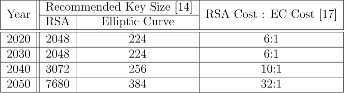
In 2012, the recommended RSA key size is 2048 bits, while it is only 224 bits for
ECC. Recommended key sizes for the year 2050 are 7680 for RSA and 384 for ECC.
Furthermore, the United States’ National Security Agency (NSA) estimates that the
computational cost of RSA compared to ECC at the current recommended security
level is 6 to 1, while this gap only increases as security requirements and key lengths
inevitably grow.
Year Recommended Key Size [14] RSA Cost : EC Cost [17]
RSA Elliptic Curve
2020 2048 224 6:1
2030 2048 224 6:1
2040 3072 256 10:1
2050 7680 384 32:1
Table 1.1: Comparison of recommended public key sizes and estimated computational cost for elliptic curve and RSA cryptography
RIM Blackberry smartphones. This is likely due to the fact that RSA was already
well-established, and also because ECC is often perceived as being patent encumbered.
Due to the combination of larger RSA key sizes, and a host of other factors well
beyond the scope of this dissertation, ECC will most likely replace RSA public key
cryptography for most applications in the coming years [18].
1.2.2
Parallel processing
As for difficulties concerning stagnant CPU clock rates, there are two major
ap-proaches the microelectronics industry is taking to put the additional transistors
afforded by process miniaturization to work. First, it has always been possible to
develop special purpose circuits to accelerate commonly used CPU tasks. As of 2008,
for example, Intel and AMD have been including special hardware to accelerate AES
block encryption, which is accessed using special instructions [19].
The second major approach for employing more transistors without significantly
increasing power consumption is parallel and massively parallel processing. It is not
uncommon for a desktop CPU to possess four or even eight physical cores, while
1.3
Research goals, and the organization of this
dissertation
The overarching goal of this work is to improve the operation throughput of elliptic
curve scalar point multiplication, which is the key operation used in all elliptic curve
cryptography algorithms. An overview of the mathematical foundation upon which
elliptic curve cryptography and elliptic curve scalar point multiplication is based is
presented in Chapter 2, along with a brief review of important cryptography protocols
and standards.
First efforts towards the acceleration of elliptic curve scalar point multiplication
began with the VLSI implementation of a recently proposed finite field reordered
nor-mal basis multiplier architecture [4], which, in turn, would lead to greatly improved
scalar point multiplication performance once integrated into a CPU or SOC. Chapter
3 presents the CMOS 0.18µm implementation of this multiplier, which uses a
com-bination of custom domino logic and standard VLSI library cells to achieve excellent
performance compared to the state of the art. In Chapter 4 the proposed finite field
multiplier was further improved upon by making some architectural changes, and
by implementing the entire design in domino logic, further reducing its critical path
delay as well as its area utilization.
The planned research goals at this stage were as follows:
1. Integrate the proposed multiplier into a CPU core, fabricate it, and measure its
results before any further improvements are carried out. This step is critical in
order to determine if there are any unforeseen issues relating to the design that
require correction, such as antenna effects, hot spots, or EM noise issues.
2. Further generalize the design so that it may carry out finite field multiplication
over a wider array of field sizes; essentially allow the proposed multiplier to be
At this point, however, some developments transpired which altered the course of this
work:
1. Practical limitations: CPUs IP cores were not (and are not) available to the
University of Windsor; this eliminates the chance to actually integrate the
pro-posed custom multiplier into a CPU design for use in accelerating cryptography
operations. Further, it is impractical to design a custom CPU capable of
run-ning even a very minimalist operating system. The ultimate goal of integrating
a custom multiplier design into a common CPU is thus out of reach.
2. Limited library components: fabricating and testing the multiplier on its own at
the high operating speeds for which it was designed requires components such
as the phase locked loops (PLLs) or delay locked loops (DLLs), which are not
available in any available library. Creating these components is possible, but
time consuming and not considered a research problem.
3. A new and interesting avenue of research for improving scalar point
multipli-cation was made available: graphic processing unit (GPU) acceleration. Until
recently, GPUs were used almost exclusively to render graphics for computer
games. Now, however, it is possible to use them to accelerate general
pur-pose computations. This aligned well with the major goal of this dissertation,
which is to determine a practical way to accelerate the performance of elliptic
curve scalar point multiplication, and as such, the remainder of this dissertation
focuses on this new and interesting area of research.
Chapter 5 presents a review GPU computing, and following this Chapter 6
pro-poses a type-II optimal normal basis multiplication algorithm for the GPU. Compared
to other GPU-based binary extension field multiplication algorithms, the proposed
per second, however it is not able to surpass a CPU implementation which makes use
of some recently released special-purpose instructions.
Noting that the GPU possesses extremely efficient integer multiplication, attention
was refocused on developing prime field multiplication algorithms. Chapter 7 presents
a NIST-fields multiplication algorithm for GPU that, to the best of the author’s
knowledge, is the fastest CPU or GPU based multiplication algorithm reported in
the literature.
In Chapter 8, a number of analyses were performed on the multiplication stage
used by the NIST multiplication algorithm, and it was determined that a very high
throughput Montgomery multiplication algorithm could be developed which
main-tains high operation throughput while allowing reduction over any finite field. This
chapter proposes a complete finite field arithmetic library based on the Montgomery
multiplication algorithm, which includes a finite field inversion algorithm based on
Fermat’s little theorem that is suitable for GPU implementations. The resulting
li-brary’s operation throughput performance is analyzed and compared to the state of
the art.
Chapter 9 presents the proposed GPU-based elliptic curve scalar point
multipli-cation algorithm, along with a series of performance analyses which characterize the
proposed in terms of operation throughput, latency, and batch size requirements.
The proposed scalar point multiplication is compared to the state of the art, and it
is shown that it boasts between 5x and 31x greater operation throughput than the
next best CPU implementation, and 6x to 7.7x greater operation throughput than
the state-of-the-art FPGA implementation.
Finally, the contributions of the work presented in this dissertation are highlighted
Mathematical Preliminaries
2.1
Introduction
The main goal of the work presented in this dissertation is to improve the operation
throughput of the elliptic curve scalar point multiplication operation that is used in
internet security protocols such as TLS and SSL which employ elliptic curve
cryp-tography algorithms. As shown in Figure 2.1, scalar point multiplication depends
on point addition and point doubling operations, which in turn require fundamental
finite field arithmetic operations such as multiplication, addition, subtraction,
squar-ing, and inversion.
This chapter presents a brief, bottom-up summary of elliptic curve cryptography,
beginning with its underlying finite field arithmetic (the bottom of the hierarchy in
Figure 2.1), followed by elliptic curve group law, scalar multiplication, and high-level
elliptic curve cryptography algorithms, which is second from the top in Figure 2.1.
fol-TLS / SSL
ECC Algorithms
Scalar Point Multiplication
Point Addition, Point Doubling
Finite Field Arithmetic Operations
Figure 2.1: Hierarchy of operations for implementing internet security protocols with elliptic curve cryptography
lowed by finite fields and extension fields in sections 2.4 and 2.4.2. In section 2.4.4
several important bases for binary extension fields are presented and compared.
Sec-tion 2.4.6 summarizes the different fields and bases used in the work presented in
this dissertation. Following this, elliptic curves and the elliptic curve group law is
introduced in section 2.5. Section 2.6 presents scalar point multiplication, and 2.8
reviews the high level protocols that ultimately carry out security services. Section
2.9 presents some concluding remarks.
2.2
Groups
A group is defined as a setGtogether with an operator ‘•’ that combines two elements
in G to form a third element also in G, and satisfies the following four properties
[20]:
Property 2.1 (Closure)
a, b ∈ G implies that a•b ∈ G
Property 2.2 (Associativity)
a, b, c, ∈ G implies that a•(b•c) = (a•b)•c
Property 2.3 (Identity element)
Property 2.4 (Inverse element)
For every a ∈ Gthere exists an element a−1 ∈ Gsuch that a•a−1 =a−1•a= 0
Abelian groups
An abelian group is a group that also satisfies the commutativity property:
Property 2.5 (Commutativity)
A group Gis said to be abelian (commutative) if for every a, b, ∈ G, a•b =b•a
The most common example of a group is perhaps the integers (ℵ) together with the
addition (+) operation.
2.3
Fields
A field is a setFtogether with two operators, often denoted as•and∗which combine
two elements in F to form a third element in F that satisfies the following seven
properties in addition to the five abelian group properties [21]:
Property 2.6 (Closure under multiplication)
a, b ∈ F implies that a∗b ∈ G
Property 2.7 (Associativity of multiplication)
a, b, c, ∈ F implies that a∗(b∗c) = (a∗b)∗c
Property 2.8 (Distributivity)
a∗(b•c) =a∗b•a∗ca for a, b, c ∈ F
(a∗b)•c=a∗b•a∗ca for a, b, c ∈ F
Property 2.9 (Commutativity of multiplication)
a∗b =b∗a for a, b, ∈ F
Property 2.10 (Multiplicative identity)
Property 2.11 (No zero divisors)
If a, b ∈ F and a∗b= 0, then either a= 0 or b = 0
Property 2.12 (Multiplicative inverse element)
Ifa ∈ Fanda6= 0, then there is an elementa−1 inGsuch thata∗a−1 =a−1∗a = 1
An example of a field is the set of real numbers<, together with the standard addition
(+) and multiplication (×) operations.
2.4
Finite fields
A finite field possesses all the properties of a field, with the additional constraint that
its set contains afinite number of elements [22].
2.4.1
Prime fields
The set of integers [0, p−1] for p prime, together with field operations defined as
addition and multiplication modulo p, form a finite field which is denoted as either
Fp or equivalently as GF(p), in honour of Evariste Galois [23]. The field prime ‘p’ is
called the characteristic of the field, and the number of elements in the field (more
properly stated as the field order) is also p. The fields GF(p) for different primes p
may also be referred to as the prime fields.
2.4.2
Extension fields
It is possible to create anm-dimensional vector space from the elements inFp, which is
equivalently denoted as eitherFpm or GF(pm). This vector space is called an extension
field, and it has a field order ofpm, and characteristicp. It can be shown thatall finite
fields are isomorphic (structurally equivalent) to Fpm, and there are many different,
vectors that span the space, allowing for different implementation advantages and
disadvantages [20].
2.4.3
Polynomial basis arithmetic
The most common basis for extension fields is polynomial (or standard) basis. In
this case, the elements are polynomials of degree at most m−1 with coefficients in
Fp, and operations are polynomial addition and multiplication modulo a primitive
degree-m polynomial [20]. Ifα is a root of the degree-m primitive polynomial which
defines the field, a polynomial can be defined as [20]:
{1, α, α2, . . . , αm−1} (2.1)
and an elementA in GF(pm) can be represented as
A={a0+a1α+a2α2+. . .+am−1αm−1} ai ∈ Fp,0≤i < m (2.2)
or equivalently using sigma notation as
A=
m−1
X
i=0
aiαi, ai ∈ Fp (2.3)
A particularly important family of extension fields are the characteristic-2 or
bi-nary extension fields, denoted asF2m, or GF(2m). Binary extension fields are of great
interest as they are especially well suited for implementation using the binary logic
employed by virtually all computer hardware. In this case, the coefficients of A in
Equation 2.3 are either 0 or 1, and adding elements A and B in a field over GF(2)
is simply an m-bit wide exclusive-or (XOR) operation. Note that this is a carry-less
operation, allowing for easy parallel implementation. As previously stated,
the primitive polynomial that defines the field. While there may exist more than one
primitive polynomial over a field GF(pm) for a specific ‘p’ and ‘m’, these different
polynomials construct fields that are structurally equivalent or isomorphic with
re-spect to each other. It is possible, however, that certain primitive polynomials lead
to more efficient implementations, such as the use of all-one polynomials (AOPs), or
equally spaced polynomials (ESPs) [24, 25].
Polynomial basis is especially popular for software implementations; compared to
alternative bases (such as those presented in the next section), they require far fewer
multi-machine-word shift operations, and fewer instructions overall. Emphasizing
the popularity of polynomial basis for software implementations, Intel has recently
included a special, dedicated instruction “PCLMULQDQ”, which is included in the
majority of their desktop and server CPUs released since 2010, can be used perform
polynomial basis multiplication very efficiently [26].
Although there are a number of different polynomial basis arithmetic algorithms
exist for both hardware and software platforms, they are beyond the scope of this
work, which concentrates on prime fields, as well as other bases in GF(2m), such
as normal basis, Gaussian normal basis, and reordered normal basis, which possess
numerous advantages in hardware and parallel implementations.
2.4.4
Normal basis, optimal normal basis, & Gaussian
nor-mal basis
A basis ofF2m overF2 of the formN ={β2
0
, β21, β22, . . . , β2m−1}for an appropriate
choice of β ∈ F2m is called a normal basis (NB) [22]. A normal basis can be
found for every finite field F2m [22]. Field elements can be represented as an
m-dimensional ordered set (a0, a1, . . . , am−1), with coefficients ai in F2, and basis
N = {β, βq, βq2
, . . . , βqm−1
} spanning F2m; this is shown compactly using sigma
represented with an array of dm
we w-bit binary words, whose bits are interpreted as
the coefficients ai in Equation 2.4.
A=
m−1
X
i=0 aiβ2
i
(2.4)
Normal basis addition over binary extension fields is carried out using the same
m-wide XOR operation used by polynomial basis. A squaring operation is especially
inexpensive in NB, as it consists of a single circular shift operation, which can be
implemented in hardware at virtually no cost. Multiplication is more complicated,
and requires a combination of circular shift, and logicical XOR and AND operations.
Normal basis multiplication
Given two elements A and B in normal basis defined as in Equation 2.4, a third
element C can be computed as shown in Equation 2.6:
C =A×B =
m−1
X
i=0 aiβ2
i
×
m−1
X
j=0 bjβ2
j
(2.5)
=
m−1
X
i=0
m−1
X
j=0
aibjβ2
i
β2j (2.6)
=
m−1
X
k=0 ckβ2
k
(2.7)
Note that the product of the double sum Pmi=0−1Pmj=0−1β2i
β2j
in Equation 2.6 must
map to the single sum Pmi=0−1β2k
in Equation 2.7. It is possible to create a
multipli-cation table λijk for each combination of i, j in Equation 2.6 to determine the sum
Pm−1
i=0 β2 k
; one method of generatingλijkis presented in [27]. Shown in the five
right-most columns of Table 2.1 is the multiplication table λijk for the finite field GF(25)
α is a root of the primitive polynomial.
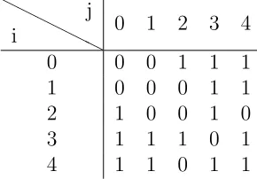
Table 2.1: Normal basis multiplication table forF25 with primitive polynomial
x5+x4 +x2+x+ 1, and β =α11 where α is a root of the primitive polynomial
i j β
2i
β2j
β2k
=β2i
×β2j
β24 β23 β22 β21 β20 β24 β23 β22 β21 β20 β24 β23 β22 β21 β20
0 0 0 0 0 0 1 0 0 0 0 1 0 0 0 1 0
0 1 0 0 0 0 1 0 0 0 1 0 0 1 1 1 0
0 2 0 0 0 0 1 0 0 1 0 0 1 0 1 1 1
0 3 0 0 0 0 1 0 1 0 0 0 1 1 1 0 1
0 4 0 0 0 0 1 1 0 0 0 0 0 0 1 1 1
1 0 0 0 0 1 0 0 0 0 0 1 0 1 1 1 0
1 1 0 0 0 1 0 0 0 0 1 0 0 0 1 0 0
1 2 0 0 0 1 0 0 0 1 0 0 1 1 1 0 0
1 3 0 0 0 1 0 0 1 0 0 0 0 1 1 1 1
1 4 0 0 0 1 0 1 0 0 0 0 1 1 0 1 1
2 0 0 0 1 0 0 0 0 0 0 1 1 0 1 1 1
2 1 0 0 1 0 0 0 0 0 1 0 1 1 1 0 0
2 2 0 0 1 0 0 0 0 1 0 0 0 1 0 0 0
2 3 0 0 1 0 0 0 1 0 0 0 1 1 0 0 1
2 4 0 0 1 0 0 1 0 0 0 0 1 1 1 1 0
3 0 0 1 0 0 0 0 0 0 0 1 1 1 1 0 1
3 1 0 1 0 0 0 0 0 0 1 0 0 1 1 1 1
3 2 0 1 0 0 0 0 0 1 0 0 1 1 0 0 1
3 3 0 1 0 0 0 0 1 0 0 0 1 0 0 0 0
3 4 0 1 0 0 0 1 0 0 0 0 1 0 0 1 1
4 0 1 0 0 0 0 0 0 0 0 1 0 0 1 1 1
4 1 1 0 0 0 0 0 0 0 1 0 1 1 0 1 1
4 2 1 0 0 0 0 0 0 1 0 0 1 1 1 1 0
4 3 1 0 0 0 0 0 1 0 0 0 1 0 0 1 1
4 4 1 0 0 0 0 1 0 0 0 0 0 0 0 0 1
In [28] it was shown that it is possible to use the λ table’s column k = 0, while
shifting input operands A and B in order to compute the product C = A×B. The
individual bits of C may be computed as shown in Equation 2.8:
ck = m−1
X
i=0
m−1
X
j=0
ai+kbj+kλij0 (2.8)
Optimal normal basis multiplication
The λij0 table for the complete multiplication table 2.1, is shown in Table 2.2. Note
Table 2.2: Multiplication table λij0 for the example in Table 2.1
H H
H H
H H
i
j
0 1 2 3 4
0 0 0 1 1 1
1 0 0 0 1 1
2 1 0 0 1 0
3 1 1 1 0 1
4 1 1 0 1 1
table’scomplexity, and is denoted CN; when Equation 2.8 is expanded, it will require
CN terms. Different normal bases may have different complexities, and it would be
advantageous to use the normal basis with the minimum possible complexity in order
to reduce the number of terms in the expanded form of Equation 2.8.
Mullin et al. did exactly this, and determined that the minimum complexity of
a normal basis over a field F2m is CN = 2m−1 [28]. Additionally, they determined
when such a basis exists, and how to construct such a basis, which is referred to as
an optimal normal basis (ONB) [28]. The authors also note that there are two types
of ONB; in practice only type-II ONB is used, as type-I ONB only exist for certain
even extension degrees (m), as there is some concern that there may be undiscovered
methods that exploits for fields with even extension degrees.
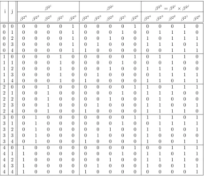
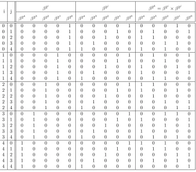
To highlight the importance of ONB, Table 2.3 presents the complete
multipli-cation table for the type-II ONB for the same field shown in the previous example,
f(x) = x5+x4 +x2+x+ 1, however this time choosing β =α instead of β =α11.
This changes the complexity CN from 15 to CN = 2m− 1 = 9, greatly reducing
the number of terms in the expanded form of Equation 2.8; the difference between a
randomly chosen NB and an ONB grows significantly for the larger field sizes that
Table 2.3: Type-II optimal normal basis multiplication table for F25 with
primitive polynomial α5+α4+α2+α+ 1, and β =α
i j β
2i β2j β2k=β2i×β2j
β24 β23
β22 β21
β20 β24
β23 β22
β21 β20
β24 β23
β22 β21
β20
0 0 0 0 0 0 1 0 0 0 0 1 0 0 0 1 0
0 1 0 0 0 0 1 0 0 0 1 0 0 1 0 0 1
0 2 0 0 0 0 1 0 0 1 0 0 1 1 0 0 0
0 3 0 0 0 0 1 0 1 0 0 0 0 0 1 1 0
0 4 0 0 0 0 1 1 0 0 0 0 1 0 1 0 0
1 0 0 0 0 1 0 0 0 0 0 1 0 1 0 0 1
1 1 0 0 0 1 0 0 0 0 1 0 0 0 1 0 0
1 2 0 0 0 1 0 0 0 1 0 0 1 0 0 1 0
1 3 0 0 0 1 0 0 1 0 0 0 1 0 0 0 1
1 4 0 0 0 1 0 1 0 0 0 0 0 1 1 0 0
2 0 0 0 1 0 0 0 0 0 0 1 1 1 0 0 0
2 1 0 0 1 0 0 0 0 0 1 0 1 0 0 1 0
2 2 0 0 1 0 0 0 0 1 0 0 0 1 0 0 0
2 3 0 0 1 0 0 0 1 0 0 0 0 0 1 0 1
2 4 0 0 1 0 0 1 0 0 0 0 0 0 0 1 1
3 0 0 1 0 0 0 0 0 0 0 1 0 0 1 1 0
3 1 0 1 0 0 0 0 0 0 1 0 1 0 0 0 1
3 2 0 1 0 0 0 0 0 1 0 0 0 0 1 0 1
3 3 0 1 0 0 0 0 1 0 0 0 1 0 0 0 0
3 4 0 1 0 0 0 1 0 0 0 0 0 1 0 1 0
4 0 1 0 0 0 0 0 0 0 0 1 1 0 1 0 0
4 1 1 0 0 0 0 0 0 0 1 0 0 1 1 0 0
4 2 1 0 0 0 0 0 0 1 0 0 0 0 0 1 1
4 3 1 0 0 0 0 0 1 0 0 0 0 1 0 1 0
4 4 1 0 0 0 0 1 0 0 0 0 0 0 0 0 1
Gaussian normal basis
Unfortunately, an optimal normal basis does not exist for all field sizes, which limits
its use compared to polynomial basis, where a primitive pentanomial or trinomial
can always be found. To ameliorate this, Ash et al. developed the concept of
type-T Gaussian normal bases (GNB), and demonstrated that type-I and II GNB are
equivalent to type-II and II ONB [29]. Higher types GNB are more computationally
expensive (or require greater hardware resources) compared to lower types, however
they guarantee the lowest complexity possible for a given field F2m. A type-T GNB
2.4.5
Reordered normal basis multiplication
Reordered normal basis (RNB) was proposed by Wu et al. [4], using some ideas from
Gao et al.[31]. RNB is a permutation of type II ONB; the complexity of RNB is
equivalent to that of ONB, however RNB allows for very regular multiplier
architec-tures which are especially amenable to hardware implementations, as signal routing
is greatly simplified. Specifically, RNB multiplication is carried out using Equation
2.14, whose derivation shown below is reproduced here from [4] for completeness.
Theorem 2.1
Letβ be a primitive (2m+ 1)stroot of unity in
F2m and γ =β+β−1 generates a type
II optimal normal basis. Then{γi, i= 1,2, . . . , m}withγi =βi+β−i =βi+β2m+1−i,
i= 1,2, . . . , m is also a basis in F2m
Forβ ∈ F2m and γi as defined in theorem 2.1, define
s(i)=4
imod 2m+ 1, if 06imod 2m+ 16m,
2m+ 1−imod 2m+ 1, otherwise
(2.9)
Now, s(0) = 0, s(i) = s(2m+ 1−i), and γi = γs(i) for any integer i. As γiγj =
γi+j +γi−j, thus γi·γj =γs(i+j)+γs(i−j). Let B = (b1, . . . , bm) ∈ F2m with respect
to the basis [γ1, γ2, . . . , γm] and b0 = 0 then
γi·B = m X
j=1
bjγi·γj = m X
j=1
bj(γs(i+j)+γs(i−j)) (2.10)
=
m X
j=1
(bs(j+i)+bs(j−i))γj (2.11)
The final step in the equation above comes from proper substitutions of the subscript
variables. The above constant multiplication γi ·B was proposed by Gao et al. in
F2m with respect to the basis [γ1, γ2, . . . , γm], then multiplication of A and B can
proceed as follows:
A·B =
m X
i=1
ai(γi·B) = m X i=1 ai m X j=1
(bs(j+i)+bs(j−i))γj (2.12)
= m X j=1 Xm i=1
ai(bs(j+i)+bs(j−1))
γj (2.13)
If the product is written as C=Pmj=1cjγj, then
cj = m X
i=1
ai(bs(j+i)+bs(j−i)), j = 1,2, . . . , m (2.14)
The λ table required for NB and ONB multiplication is irregular, and varies
with different fields F2m and choices for element β, which can complicate hardware
designs by adding to routing overhead. This also causes software algorithms to require
irregular memory access patterns. RNB multiplication using Equation 2.14 does not
require such a table, and some very regular hardware architectures have been proposed
to take advantage of this property [4]. RNB squaring requires a simple permutation of
the bits making up the operands, which is implemented inexpensively in hardware by
“shuffling” wires. Software implementations of RNB squaring could be significantly
more expensive without dedicated hardware such as a multi-precision barrel shifter.
2.4.6
Summary of finite fields
Figure 2.2 presents a simple taxonomy of the finite fields presented in this section.
To summarize, all finite fields are of the form Fqm for prime q. If q = 1, the finite
field may be referred to as a prime field; its elements are the integers, and the field
operations are integer multiplication and addition modulo the field primep. Ifq >1,
q = 2 are of particular interest due to their compatibility with boolean logic; these
are called binary fields.
Finite Fields
Prime Fields Extension Fields
Binary Extension Fields
Normal Basis Polynomial Basis
Gaussian Normal Basis
Optimal Normal Basis Reordered Normal Basis
Figure 2.2: Taxonomy of finite fields and bases
Binary fields may be expressed using a number of different bases which are
equiv-alent or isomorphic. The different bases discussed in this dissertation are shown in
the shaded part of Figure 2.2, and the bi-directional arrows denote that the bases
are isomorphic with respect to each other. Polynomial basis is often used for
soft-ware implementations of binary fields as it requires fewer shifting operations and
pre-computations compared to normal basis. Normal basis, which is isomorphic to
polynomial basis, is considered inefficient, however a Gaussian normal basis can be
found for most applications which significantly reduces the complexity of the
multi-plication operation. Type-I and type-II Gaussian normal bases are equivalent to an
optimal normal basis, which has the least complex multiplication operation of any
normal basis. Optimal normal basis only exist for a fraction of possible field sizes,
however. Finally, reordered normal basis is a permutation of type-II optimal normal
2.5
Elliptic curves and elliptic curve group law
Elliptic curves, named as such due to their relationship with elliptic integrals, are
defined as the locus of rational points P = (x, y), with x, y elements of some field of
characteristic6= 2,3 which satisfiesy2 =x3+ax+b, ∆ =−16(4a3+27b2)6≡0, together
with the point at infinity “O” [32]. In the case where the field is of characteristic
2 (i.e. the binary extension fields) an elliptic curve is the locus of points satisfying
y2 =x3 +ax2 +bx+c together with the point at infinity O, for a, b, and c ∈
F2m
[33].
The elliptic curvey2 =x3+x+ 3 over <(an infinite field) is shown in Figure 2.3a.
Elliptic curves may be defined over any field, including finite fields; the same curve
(y2 =x3+x+ 3) over the finite field F11 is shown in Figure 2.3b.
−6 −4 −2 0 2 4 6
−6 −4 −2 0 2 4 6 (a)
0 1 2 3 4 5 6 7 8 9 10
0 1 2 3 4 5 6 7 8 9 10 (b)
Figure 2.3: The elliptic curve y2 =x3+x+ 3 over (a) the infinite field <and (b)
over the finite field F11
Elliptic curve group law
It is possible to define a group law using elliptic curves. For rational points P(x, y)
and point at infinity O on the elliptic curveE over a field Fp, the point O at infinity
is the identity element, meaning P +O =P. Negatives are formed by changing the
For two points P and Q on the elliptic curve, P 6= Q, addition P +Q is performed
by tracing a line between P and Q, finding the point where the line intersects the
elliptic curve, and then reflecting that point about the x-axis, as shown in Figure
2.4a. This may also be written as shown in Equation 2.15, where P = (x1, y1), Q=
(x2, y2), Q, P ∈ E, P 6=Q and P +Q= (x3, y3).
x3 =
y2−y1
x2−x1
2
−x1−x2 and y3 =
y2−y1
x2−x1
(x1−x3)−y1 (2.15)
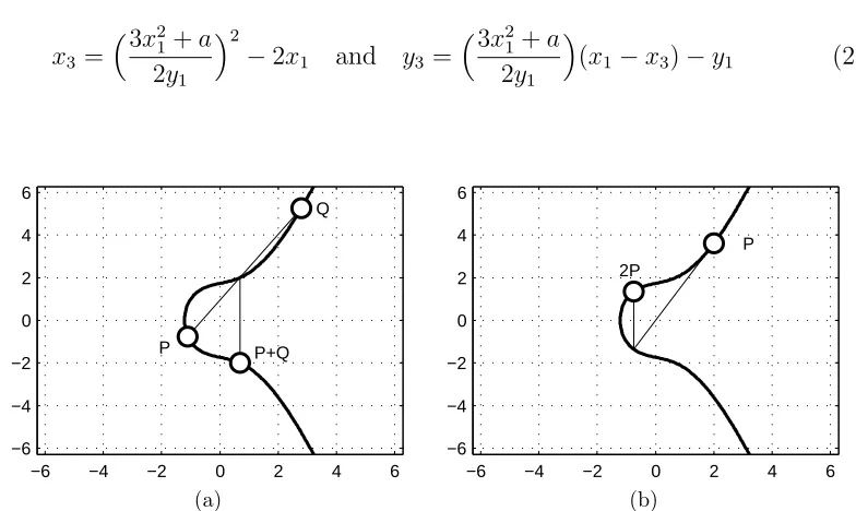
In the event P =Q, a point doubling equation is used to compute 2P: a line tangent
toP is drawn, and the point where the line intersects the elliptic curve is found, and
reflected about thex-axis as shown in Figure 2.4b. This may also be written as shown
in Equation 2.16, where P = (x1, y1), P ∈ E, and 2P = (x3, y3).
x3 =
3x2
1+a
2y1
2
−2x1 and y3 =
3x2
1+a
2y1
(x1−x3)−y1 (2.16)
−6 −4 −2 0 2 4 6
−6 −4 −2 0 2 4 6 P Q P+Q (a)
−6 −4 −2 0 2 4 6
−6 −4 −2 0 2 4 6 P 2P (b)
Figure 2.4: (a) Elliptic curve point addition and (b) doubling over the infinite field<
Note that while the above formulas are for prime fields, similar formulas also exist
Elliptic curve group order
Another important aspect of elliptic curve groups over finite fields is their grouporder,
that is, the number of rational points that exist on the elliptic curve. The order n
can be estimated using Hasse’s theorem which states that for a finite field Fq:
q+ 1−2√q≤n≤q+ 1 + 2√q (2.17)
2.6
Scalar Point Multiplication and the Elliptic
Curve Discrete Logarithm Problem
With a rule for the addition and doubling of points on an elliptic curve, it is possible
to define scalar point multiplication over an elliptic curve E of order n over a finite
field Fpq as the repeated addition of an elliptic curve point:
Q=kP, for Q, P ∈ E and k ∈ [0, n−1] (2.18)
=P +P + . . . +P (k times) (2.19)
Given an elliptic curve E of order n, a base point P on the curve, and a scalar
k ∈ [0, n−1], it is possible to compute Q=kP using an algorithm such as
double-and-add. Computing k with knowledge of the curve, Q, and P, on the other hand
is believed to be intractable and computationally unfeasible for curves with large
order n; this is the elliptic curve discrete logarithm problem (ECDLP) upon which
elliptic curve cryptography is based. It is worth noting that the ECDLP has not
been proven to be an NP-hard problem [34]. The best known algorithm to solve
or attack the ECDLP is the “Pollard Rho” method which requires approximately
p
2.7
Elliptic curve cryptography protocols
While elliptic curve cryptography protocols are beyond the scope of this dissertation,
a brief overview of the elliptic curve Diffie-Hellman key exchange and the elliptic
curve digital signature algorithm are provided to give a context for how scalar point
multiplication is used, and the various standards that specify the various elliptic
curve cryptography parameters. Both of these algorithms are based on the ECDLP
described in the previous section.
2.7.1
Elliptic curve Diffie-Hellman exchange
The elliptic curve Diffie-Hellman key exchange (ECDH) is used when Alice (A) and
Bob (B) need a shared secret, which is often used as a key for a much faster symmetric
block encryption algorithm such as AES. The ECDH exchange is described as follows,
and more details are provided in [35]:
Alice and Bob must first agree to a set of elliptic curve parameters: the field sizem
for binary fields (or the field primepfor fieldsFp), the specific elliptic curveEof order
n, and a base point G ∈ E. Alice and Bob also select two different random values
dA and dB in the interval [0, n−1]. Only Alice knows dA, and only Bob knows dB;
these values serve as Alice and Bob’s private keys. Finally, Alice and Bob compute
QA=dAG and QB =dBG, respectively, where QA and QB serve aspublic keys.
In order to exchange a shared secret, Alice and Bob exchange QA and QB. Alice
now computesdAQBand Bob computesdBQA. SincedAQB =dA(dBG) =dB(dAG) =
dBQA, Alice and Bob now have a shared secret. Also, because only Bob knows dB
and only Alice knows dA, any third party intercepting QA and QB will not be able
to reconstruct the shared secret without attacking the ECDLP. It should be noted
that generating a public/private key pair requires multiplying a fixed point G on an
scalar multiplication of an unknown point.
2.7.2
Elliptic Curve Digital Signature Algorithm
Another major function public key cryptography performs is digital signature, which
is used to assert the identity of the author of a message and prevents the message
itself from being altered. Two separate algorithms are used in the elliptic curve digital
signature algorithm (ECDSA), one for signing a message (algorithm 2.1), the other
for verifying it (algorithm 2.2).
Algorithm 2.1: ECDSA Signature Generation [35]
input : Elliptic curve parameters a, b, base point P, curve ordern, the field
Fqm, private keyd, message m
output: Signature (r,s)
1 Select k ∈ [1, n−1]
2 Compute kP = (x1, y1)
3 Compute r =x1 mod n; if r = 0 go to step 1
4 Compute e = hash(m)
5 Compute s =k−1(e+dr) mod n; if s= 0 go to step 1
6 Return (r, s)
Algorithm 2.2: ECDSA Signature Verification [35]
input : Elliptic curve parameters a, b, base point P, curve ordern, the field
Fqm, public key Q, message m, signature (r,s)
output: Acceptance or rejection of the signature
1 Verify that r and s are integers in the interval [1, n−1], if not then return
“signature rejected”
2 Compute e = hash(m)
3 Compute w=s−1 mod n
4 Compute u1 =ew mod n and u2 =rw mod n
5 Compute X =u1P +u2Q
6 If X =O (the point at infinity), return “signature rejected”
7 Compute v =x1 mod n
8 If v =r return “signature accepted”, otherwise return “signature rejected”
unknown scalar point multiplication, while verifying it with algorithm 2.2 must
com-pute the sum of two scalar point multiplications.
2.8
Elliptic curve cryptography standards
To date, a number of standards have been defined for elliptic curve cryptography
which specify the underlying field size and elliptic curve parameters. Note that while
these standards specify how key exchange and signature operations are to be carried
out, implementation details are left up to hardware and software engineers.
Among the most important is the National Institute of Standards and Technology
(NIST) Federal Information Processing Standards Publication 186-3 (FIPS 186-3)
[35]. This standard defines the approved algorithms for digital signature, which
in-cludes DSA (which uses the RSA algorithm) and ECDSA. Additionally, FIPS 186-3
defines specific prime moduli, associated elliptic curves, and elliptic curve base points
to be used for ECDSA. The five prime moduli defined by this standard are of special
form that allow for simplified arithmetic on computer hardware with machine word
sizes of 32 bits. The associated elliptic curves’ “a” parameters are fixed at −3 mod
p, as this allows for a slightly more efficient elliptic-curve point doubling operation,
while the curves’ “b” parameters are pseudo-randomly chosen.
FIPS 186-3 also defines five binary extension fields that are roughly equivalent in
security to the prime fields. The field sizes are chosen such that a Gaussian Normal
Basis exists, and the field polynomial (either a trinomial or pentanomial) is specified.
For each of these binary extension fields, two curves are specified: one is chosen
pseudo-randomly, while the other is a “Koblitz” or anomalous binary curve. Koblitz
curves have some properties that allow for efficient implementations, however they
are beyond the scope of this dissertation.
X9.62 [30] and X9.63 [36], which detail the algorithms and data structures to be used
in the financial services industry to carry out elliptic curve key exchange and digital
signature, respectively. Note that these standards specify only the algorithms and
data structures, and not which fields or elliptic curve parameters to use.
The United States’ National Security Administration (NSA) “Suite B” specifies
an entire suite of cryptographic protocols to secure communication up to a “Top
Secret” security level [16]. Suite B requires the use of the 256 or 384 bit prime field
(and associated elliptic curves and algorithms) specified NIST’s FIPS 186-3 standard
for digital signature. For key exchange, Suite B uses algorithms specified in the NIST
Special Publication 800-56A with the fields and curves specified in FIPS 186-3.
The standards for efficient cryptography group (SECG) has their own standard
[37], which is a superset of the FIPS 186-3 standard: in addition to the curves and
fields defined in the NIST standard, it also defines at set of “prime” Koblitz curves
which allow for some advantages conducting scalar point multiplication, however there
is some concern that these curves might also have some still-unknown vulnerabilities
[38].
The IEEE has its own standard titled “IEEE P1363”, which specifies a number
of acceptable algorithms for use in key exchange, digital signature, as well as block
encryption. Per the standard, a number of elliptic curve cryptography algorithms
may be used including ECDH, ECDSA, as well as some less common ones such as
MQV and El-Gamel [39].
The Brainpool Standard Curves are a group of curves specified by a German group
[40]. Unlike the NIST curves, they deliberately use randomly chosen field primes and
field polynomials, and the elliptic curve parametersaandbare both randomly chosen
as well. The primes and curve parameters are random to avoid any undisclosed or
not-yet-discovered exploitation of the NIST primes, or by setting the elliptic curve
2.9
Summary
Security protocols based on elliptic curve cryptography rely on a hierarchy of
oper-ations. At the base of this hierarchy are finite field operations which can be
imple-mented using different bases that have different advantages and disadvantages that
depend on the implementation.
Rational points on an elliptic curve over finite fields form a group, where the group
operation is defined using a chord-and-tangent rule.
Scalar elliptic curve point multiplication can be used to implement public key
cryptography services based on the elliptic curve discrete logarithm problem, such as
key exchange and digital signature. Elliptic curve cryptography requires much smaller
key sizes compared to RSA, and some standards have replaced the use of RSA with
A High-Speed Implementation of a SIPO Multiplier Using RNB
3.1
Introduction
As described in Chapter 1, section 1.3, there are a number of approaches suitable
for improving the performance of elliptic curve scalar point multiplication. In turn,
scalar point multiplication is dependent on the performance of its underlying field
operations. Figure 3.1 presents estimated upper and lower bounds of the different
finite field operations required for a single scalar point multiplication over varying field
sizes. It is quickly revealed that finite field multiplication has the highest count, while
it was seen in Chapter 2 that it is also more computationally expensive than addition
or squaring. Improving finite field multiplication will directly lead to improved scalar
point multiplication performance.
150 200 250 300 350 400 450 500 0
2000 4000 6000 8000
Field Size
Operation Count
Multiplications
(a) Number of finite field multiplications per scalar point multiplication
150 200 250 300 350 400 450 500
0 2000 4000 6000 8000
Field Size
Operation Count
Squarings
(b) Number of finite field squarings per scalar point multiplication
150 200 250 300 350 400 450 500
0 2000 4000 6000 8000
Field Size
Operation Count
Addition/subtractions
(c) Number of finite field additions & subtractions per scalar point multiplication
Figure 3.1: Estimated range of finite field operation counts for scalar point multiplication over different field sizes
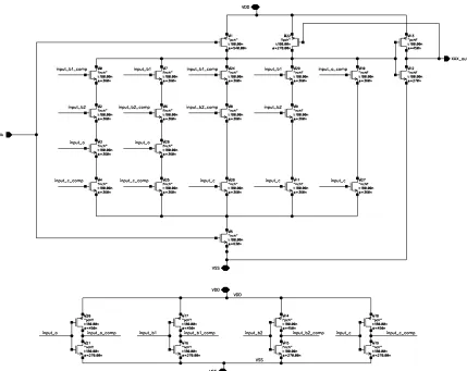
Proposed in this chapter is a a new VLSI implementation for a Serial-In
be integrated into a CPU or SOC, enabling special finite field multiplication
instruc-tions to accelerate the performance of elliptic curve scalar point multiplication.
The multiplier was implemented in a.18µmTSMC CMOS technology using
multi-ples of a custom-designed domino logic block. The domino logic design was simulated,
and functioned correctly up to a clock rate of 1.587 GHz, yielding a 99% speed
im-provement over the static CMOS’ simulation results, while the area was reduced by
49%. This multiplier’s size of 233 bits is currently recommended by NIST for ECDSA
and ECDH algorithms, and is of practical size for use for binary field multiplication
in elliptic curve cryptosystems.
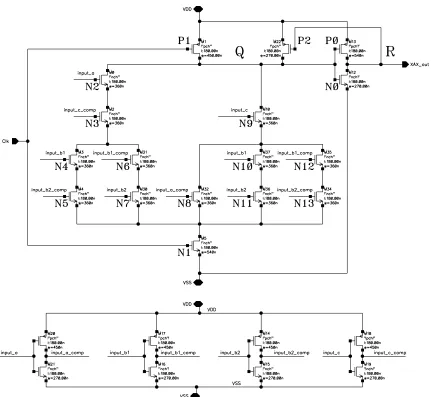
The organization of this chapter is as follows: Section 3.2 presents a survey of
existing architecture for type-II ONB multiplication. In section 3.3, the design and
implementation of the xax-module which is the main building block of the multiplier,
is discussed. Section 3.4 presents the implementation of a 233-bit multiplier using the
xax-module as the main building block. In section 3.5, comparisons between different
VLSI implementations are presented. A few concluding remarks are given in section
3.6.
3.2
A review of existing architectures for ONB
type-II multiplication
As described in Chapter 2, section 2.4.5, the type II ONB and reordered normal basis
representations of an element are simple permutations of each other. Therefore, RNB
multipliers can be used as type-II ONB multipliers and vice versa. Many different
architectures have been proposed for multiplication in normal basis, and most
archi-tectures fall into one of three main categories: bit-serial, bit-parallel, and word-serial.
Bit-serial multipliers requiremclock cycles to compute anm-bit wide multiplication.

![Figure 3.2: Serial-In Parallel-Out RNB multiplier [4]](https://thumb-us.123doks.com/thumbv2/123dok_us/1434479.1175885/58.612.148.494.460.693/figure-serial-in-parallel-out-rnb-multiplier.webp)