Performance Analysis of Large-Scale MU-MIMO
With a Simple and Effective Chanel Estimator
Felipe A. P. de Figueiredo
‡∗, Claudio F. Dias
‡, Eduardo R. de Lima
†and Gustavo Fraidenraich
‡ ∗Ghent University - imec, IDLab, Department of Information Technology, Ghent, Belgium.
†
Eldorado Research Institute, Campinas, Brazil.
‡
DECOM/FEEC–State University of Campinas (UNICAMP), Campinas Brazil.
Email:
∗[email protected],
†[email protected],
‡[aplnx, gf]@decom.fee.unicamp.br.
Abstract—Accurate channel estimation is of utmost importance for massive MIMO systems that allow providing significant improvements in spectral and energy efficiency. In this work, we investigate the spectral efficiency performance and present a channel estimator for multi-cell massive MIMO systems sub-jected to pilot-contamination. The proposed channel estimator performs well under moderate to aggressive pilot contamination scenarios without prior knowledge of the inter-cell large-scale channel coefficients and noise power. The estimator approximates the performance of a linear Minimum Mean Square Error (MMSE) as the number of antennas increases. Following, we derive a lower bound closed-form spectral efficiency of the Maximum Ratio Combining (MRC) detector in the proposed channel estimator. The simulation results highlight that the proposed estimator performance approaches the linear minimum mean square error (LMMSE) channel estimator asymptotically.
Index Terms—Massive MIMO, Multi-Cell, Pilot-Contamination, Channel Estimation.
I. INTRODUCTION
The foreseen demand increase in data rate has triggered a research race for discovering new ways to increase the spectral efficiency of the next generation of mobile and wireless net-works [1]. The report in [1] predicts that data rates will easily reach peaks of 10 Gbps, reaching a staggering 49 Exabytes of data transfer per month. Additionally, the next generation of networks is also expected to serve a higher number of devices, including human-type communication (HTC) devices and machine-type communication devices (MTC). One of the performance requirements defined by the International Mobile Communications (IMT) requires a connection density of1×106devices/km2for a network to be considered 5G [2]. According to [3], the number of connected devices is forecast to be nearly 30 billion by 2023, where around 20 billion are forecast to be MTC devices.
In that sense, several approaches have been proposed to increase the spectral efficiency of such next-generation net-works, such as cell densification through the reduction of the cell size [4], high-order modulations such as 128-QAM or 256-QAM [5], larger transmission bandwidths available on the millimeter-wave bands and aggregation of industrial, scientific and medical (ISM) bands [6, 7] simultaneous access using a single time-frequency resource employing non-orthogonal multiple access (NOMA) through different transmission power allocation or spreading-codes [8], and simultaneous multiple
users access in the same time-frequency resources by ex-ploiting a higher number of degrees-of-freedom provided by massive MIMO techniques [9]. Among all these approaches, massive MIMO is one of the most important, prominent and studied ones, and is already established on the initial deployments of the 5-th generation of mobile networks (5G) [10].
In a multi-cell massive MIMO system, the base station (BS) has to estimate the wireless channels of all its connected devices. These channel estimates obtained during the uplink communication are used to calculate the decoding and the precoding matrices, which are used to receive and transmit user data, respectively. Therefore, accurate estimation of the channels is an essential task in such systems. The LMMSE channel estimator is optimum when it comes to MSE mini-mization [11]. However, the channel statistics at the BS must be known beforehand as a premise for the estimator to work properly, i.e., it needs to have previous knowledge of both the intra/inter-cell large-scale fading coefficients and the noise power [12].
The estimation of the intra/inter-cell large-scale fading co-efficients and noise power might be unjustified in practice due to the excessive overhead it imposes on the system [12]. For instance, in the case where there are Lcells servingK users (or MTC devices for example), each one of the L-th BSs would have to acquireK(L−1)inter-cell large-scale fading coefficients plus the noise power estimation. In the foreseen case where cells have to serve a huge number of MTC devices along with human-type communication (HTC) devices, the estimation of the inter-cell large-scale fading coefficients plus the noise power estimation becomes unfeasible.
In this work, we present a channel estimator for multi-cell multi-user systems that does not require the estimation of the inter-cell large-scale fading coefficients plus noise power. We derive closed-form lower-bound expressions for the spectral efficiency of a system employing MRC detection with MMSE and proposed channel estimation. The simulation results presented here show that the performance of the pro-posed estimator asymptotically approaches that of the LMMSE channel estimator.
II. UPLINKSIGNALMODEL
In this work, we consider a multi-cell system with L cells, each cell has a BS, and each BS operates with M
antennas and K randomly located single antennas devices. Let gilkm represents the complex channel gain from the
k-th device wik-thin k-the l-th cell to the m-th antenna of the BS located at the ith cell. The channel gain, gilkm, can be
re-written as gilkm =
√
βilkhilkm where βilk represents the
large-scale coefficients (taking into account both path-loss and shadowing) and hilkm represents a frequency-flat fading
channel coefficients. The large-scale fading coefficients from the k-th device located at the l-th cell to the ith cell, βilk,
are assumed constant for all the M antennas at the ith BS, once path-loss and shadow fading change slowly along the space [14, 15]. The channel can be considered flat Rayleigh fading as the small-scale fading is considered to follow a complex Gaussian distribution with zero mean and unitary variance and the transmitted signal’s bandwidth is smaller than the coherence bandwidth [14]. The overall channel matrix is denoted by Gil and has dimension M ×K, where its k-th
column,gilk= [gilk1,· · · , gilkM]T, represent the channel gain
from thek-th device in thel-th cell to theith BS. Additionally, we consider the set of large-scale coefficients,{βilk}, as being
deterministic during the estimation phase. This assumption is reasonable due to the slow change of large-scale fading in comparison with the small-scale fading coefficients [15]. The overall channel matrix Gil can be defined directly by the
channel coefficients as Gil =HD1/2, where His a M ×K
matrix containing the small-scale fading coefficient vectors of the K channels and Dis the diagonal matrix with the large-scale coefficients for all K devices, βilk, k= 1, . . . , K.
III. UPLINKTRAINING
We assume that the devices of all cells use the same set of pilot sequences at the same time (i.e., all devices’ transmis-sions aligns to the BS uplink) and that the pilot reuse factor is equal to one, which is the most aggressive case for pilot reuse. If we assume a static channel during coherence timeTc
then the proper signal multiplexing scheme is Time-Division Duplexing (TDD) protocol. Furthermore, we can additionally say that uplink and downlink channels are reciprocal, i.e., they are identical within the channel coherence time, which minimizes the pilot transmission overhead since only devices need to transmit pilots in the uplink direction. Therefore, two direct consequences of the TDD protocol adoption are: (i) the channel coherence time limits the TDD frames [16, 17], and (ii) the pilot overhead cost is only proportional to the number of terminals, K, and not to the number of antennas, M [18, 19]. Finally, we assume Orthogonal frequency-division duplexing multiplexing (OFDM), which is a well-known mod-ulation with a straightforward interpretation of the coherence interval concept [15].
The pilot sequences ofK devices are represented by aτ× K matrix Φ with the orthogonality property, ΦHΦ = I
K,
whereK≤τ. The received pilot sequences at theith BS are represented by a M×τ matrix,Yi, defined as
Yi=
√ ρGiiΦH
| {z }
Desired pilot signals +√ρ
L X
l=1,l6=i
GilΦH
| {z }
Undesired pilot signals + Ni
|{z}
Noise . (1)
where ρ is the average pilot transmit power of each device andNi is a M ×τ matrix with i.i.d. elements following the
distributionCN(0,1). Equation (1) clearly shows the coherent inter-cell interference, which is represented by the second term in the equation and is caused by devices employing the same pilot sequences within other BSs.
As the length of the pilot sequences has to be much smaller than the coherence time, the maximum number of orthogonal sequences within a cell is limited, and due to that, other cells end up reusing the same pilot sequences. This reuse of pilot sequences brings about what is known in the literature as pilot contamination [15]. Due to the pilot contamination phenomenon, channel estimates obtained within a given cell get contaminated by pilots transmitted by the devices located within neighbour cells. The worst-case scenario for pilot contamination is when the frequency reuse factor is equal to 1 (i.e., all cells reuse the same frequency) and all transmissions coming from the different cells are perfectly synchronized. Pilot contamination leads to the coherent interference term in Equation 1, which is hard to mitigate in the case of spatially uncorrelated channels [13]. Under this specific channel condition, pilot contamination is an impairment that does not disappear, even with an infinite number of antennas [13]. On the other hand, the coherent interference caused by pilot contamination becomes negligible when large frequency reuse factors are adopted [15].
Letφk denote thek-th column ofΦH. Hence, a sufficient
statistic for the estimation of the channel vectors,giik, at the
ith BS is given by
zik=
1 √
ρYiφk =
L X
l=1
GilΦHφk+
1 √
ρNiφk
= giik
|{z}
Desired channel +
L X
l=1,l6=i
gilk
| {z }
Inter-cell interference +wik
|{z}
Noise ,
(2)
where wik = √1ρNiφk has distribution CN(0M,1ρIM) and
zik follows the distribution CN(0M, ζikIM) where ζik =
PL
l=1βilk + 1ρ. During the detection phase, the ith BS has
to estimate the channels of its devices,i.e.,gilk,∀k, based on
the transmitted pilot sequences.
IV. CHANNELESTIMATION
In this section, we briefly present two of the most well-known and heavily used channel estimators in the Massive MIMO literature [12], namely, Least-Squares (LS) and Linear Minimum Mean-Square Error (LMMSE) channel estimators.
A. Least-Squares
A sufficient statistic for estimating the channel vectors giik,∀k at theith BS is defined as [11]
ˆ
gLSiik=zik, (3)
with distribution given byCN(0M, ζikIM)[12]. Additionally,
by using (3), we can show thatˆgLSilk = ˆg
LS
iik,∀l, meaning that the
This estimator is known as the Least Squares (LS) estimator and as can be seen, it does not rely on any prior information on the channel statistics, such as the large-scale fading coef-ficients. Moreover, the LS estimator is known to have poorer performance than the MMSE estimator [12].
B. Linear Minimum Mean-Square Error
In case the channel statistics (i.e., large-scale fading coef-ficients and noise power) are assumed perfectly known at the ith BS, the optimum LMMSE channel estimator is defined as
ˆ
gMMSEiik = βiik
ζik
zik, (4)
with distribution given byCN(0M, β2
iik
ζikIM)[12]. Additionally, by using (4), we can show that ˆgMMSEilk = βilk
βiikˆg MMSE
iik ,∀l,
meaning that the channel estimates are parallel vectors that only differ by the scaling factor, βilk
βiik.
V. A SIMPLE ANDEFFECTIVECHANNELESTIMATOR
After analyzing the LMMSE channel estimator equation, given by (4), we realize we do not need to know the individual large-scale fading coefficients plus the noise power, but, in fact, what is necessary is their summation, denoted byζik. The
term ζik can be estimated by using the maximum-likelihood
(ML) method [11] and noticing that zik ∼ CN(0M, ζikIM),
therefore a estimator for ζikis defined as
ˆ
ζik=
kzikk2
M , (5)
which hasE h
ˆ
ζik i
=ζikand var h
ˆ
ζik i
=ζ2
ik/M. The
Cramer-Rao bound of the estimator is given by
varhζˆik i
≥ζik2/M. (6)
Therefore, we conclude that the estimator of ζik is the
minimum variance unbiased estimator (MVUE) [11], i.e., it is an unbiased estimator once its mean is equal to the value being estimated and it presents the lowest variance among all other possible estimators of ζik.
After replacing ζik by ζˆik in (4), a very simple but yet
effective channel estimator for the multi-cell case is defined by
ˆ
gprop.iik =M βiik
zik
kzikk2
, (7)
which asymptotically approaches the performance of the linear LMMSE estimator asM → ∞[12].
The channel estimator presented in Equation (7) has
E[ˆgpropiik] =0M and covariance matrix given by
E[ˆgpropiik(ˆg
prop
iik) H
] =
M
M−1
β2
iik
ζik
IM. (8)
The mean of E[ˆgpropiik] is found by using the symmetry
property of the distribution of zikm ∼ CN(0, ζik), we
con-clude that Egˆpropiikm
= 0, onceE
h z
ikm
kzikk2
i
=Eh−zikm
kzikk2
i
,∀m. As can be seen by analyzing equation (8), as M → ∞, Cov[ˆgpropiik] → βiik2
ζikIM, which is the covariance matrix of the LMMSE estimator [12].
Remark 1. The average normalized squared Euclidean
dis-tance betweenˆgpropiik andˆgMMSEiik is given by
1
ME
h
kˆgpropiik −ˆgMMSEiik k2i= 1 M−1
β2
iik
ζik
=ik. (9)
The proof of (9) is given in Appendix B of [12]. Fromζik
and (9), it is easily noticeable that the average distance de-creases with increasingM, decreasingρ, increasingβilk, i6=l,
and decreasingβiik.
VI. SPECTRALEFFICIENCY
The received signal at theith BS is denoted as
yi=√ρ
L X
l=1
K X
k=1
gilkxlk+ni, (12)
wherexlk are the data symbols, which are mutually
uncorre-lated and have zero mean and unit power and ni represents
noise whose elements are i.i.d. CN(0,1). During the data transmission phase, the received signal yi ∈ CM at the ith
BS is linearly processed by vik ∈ CM, i.e., the receiving
combining vector assigned by BSito itskth device, resulting in
rk=vHikyi =
√ ρ
L X
l=1
K X
k=1
vHikgilkxlk+vHikni (13)
In order to quantify the spectral efficiency (SE) under imperfect channel statistics information, we need to use a capacity lower-bound that does not require LMMSE estimates. The use-and-then-forget (UatF) bound can be applied to the case at hand [13], where the received combined signal is re-written as
rk= √
ρEvHikgiik
xik+ √
ρ vHikgiik−E
vHikgiik
xik
+√ρ K
X
k0=1,k06=k
vHikgiik0xik0+
√ ρ
L
X
l=1,l6=i K
X
k=1
vHikgilkxlk+vHikni.
(14) By treating EvHikgiik
as a known deterministic chan-nel and noticing that the other terms are uncorrelated with
EvHikgiik
xik, then, the following result is obtained.
Lemma 1. The channel capacity of thekth device at theith BS is lower bounded by
SEik= log2(1 +γik) [bits/s/Hz], (15)
withγikgiven by
γ
ik=
ρ|E
[
vHikgiik]
|2ρPL l=1
PK
k=1E
[
|vHikgilk|2]
−ρ|E[
vHikgiik]
|2+E[kvikk2],
(16)
where the expectations are with respect to the channel real-izations.
Closed-form expressions for the lower-bound can be found with the MRC type of detection scheme, where the receiving combining vector is expressed as vik=wikzik, wherewik is
defined as
wik=
(β
iik
ζik, LMMSE estimator,
M βiik
kzikk2, Proposed estimator.
γLMMSEik =
ρM β2
iik
ζik
ρPL l=1
PK
k0=1βilk0+ρM
ζik
PL
l=1,l6=iβilk2 + 1
(10)
γikProp.=
ρ(M−1)β2
iik
ζik
ρhPL l=1
PK
k0=1,k06=kβilk0+(M−1)
(M+1)
PL
l=1βilk i
+ρMζ
ik
h(M−1)
(M+1)
PL
l=1β 2
ilk−
(M−1)
M β
2
iik i
+ 1
(11)
-10 0 10 20 30 40 50 60 70 80 90 100 [dB]
10-4 10-3 10-2 10-1
Distance between Prop. and MMSE estimators
0 1 2 3 4 5 6 7 8 9 10
1/
M = 10 M = 30 M = 100 M = 200 M = 500 1/
Figure 1. Distance between the proposed and MMSE channel estimators (Remark 1).
*
*
*
*
*
*
*
*
*
*
*
*
*
*
*
*
*
*
*
*
*
*
*
*
*
*
*
*
*
*
*
*
*
*
*
*
*
*
*
*
*
*
*
*
*
*
*
*
*
*
*
*
*
*
*
*
*
*
*
*
*
*
*
*
*
*
*
*
*
*
*
*
Base Station Devices
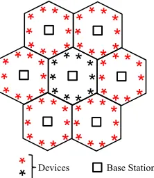
Figure 2. Multi-cell setup witlL= 7cells andK= 10devices in each cell, where each pilot is reused by the device at the same position in all cells.
After computing the expectations in (16) for the LMMSE and proposed channel estimators, then, the channel capacity of the kth device at the ith BS can be lower bounded by (15) with γik given by (10) and (11) for the LMMSE and
proposed channel estimators respectively. The proof for the LMMSE estimator can be found in [15] and for the proposed channel estimator is available in Appendix A.
Remark 2. The channel capacity of the MRC combining with the proposed channel estimator asymptotically approaches that of the MRC with the LMMSE channel estimator as the
number of antennas increases,i.e.,limM→∞γProp.ik →γ
MMSE ik .
VII. SIMULATIONRESULTS
In this section, we present simulation results assessing the performance of the proposed estimator and showing that its
30 50 100 150 200 250 300 350 400 450 500
Number of antennas, M
2 3 4 5 6 7
Spectral Efficiency [bit/s/Hz]
MMSE Simulated MMSE Analytical
30 50 100 150 200 250 300 350 400 450 500
Number of antennas, M
2 3 4 5 6 7
Spectral Efficiency [bit/s/Hz]
Prop, Simulated Prop. Analytical
Figure 3. Lower bounds and numerically evaluated values of the spectral efficiency for different numbers of BS antennas for MRC detector.
100 200 300 400 500 600 700 800 900 1000 Number of Antennas, M
2 3 4 5 6 7 8 9
Spectral Efficiency [bit/s/Hz]
0 0.5 1 1.5 2 2.5 3
Mean Absolute Percentage Error (MAPE)
MMSE Analytical Prop. Analytical
Figure 4. Sum SE achieved with MRC detector with LMMSE and proposed channel estimators over different number of antennas,M.
performance tends to that of the optimum LMMSE channel estimator.
In Figure 1, we compare the distance between the proposed and MMSE channel estimators for different number of anten-nas,M, withβiik= 1andβilk= 0.05,∀l6=i. As the Remark
1 states, the distance is small at low values of ρ, increasing with it until a ceiling value is reached. As can be also noticed, the ceiling value decreases with the number of antennas, M. The figure also depicts the variation of 1/ρ, showing that it has a direct impact on the distance as it direct affectsζik. For
lowρvalues the term β2iik
a fixed value of M.
Next, we consider the multi-cell setup depicted in Figure 2, with L= 7 cells and inter-BS distance of 2 Km. The uplink spectral efficiency is evaluated at the central cell. Each cell serves K = 10 devices at 950 m from the serving BS, in a circular pattern as showed in the figure. The devices that are located at the same position in different cells reuse the same pilot sequence. Each device has an average pilot transmit power ofρ= 20dB. The large-scale fading coefficients{βilk}
are independently generated byβilk=ψ/
d
ilk
d0
v
, wherev= 3.8,10 log10(ψ)∼ N(0, σ2
shadow,dB) withσshadow,dB = 8, and dilk is the distance of thekth device in thelth cell to theith
BS.
Figure 3 depicts the simulated spectral efficiency and the derived analytical lower bounds for the MRC detector. As it can be clearly seen, all bounds are very tight. Therefore, next, we use these bounds for the numerical work.
Figure 4 shows the sum spectral-efficiency (SE) achieved with the MRC detector with LMMSE and proposed channel estimators as a function of the number of antennas, M. The SE is evaluated at the center cell. As it can be seen, and previously showed by Remark 2, MRC detection with the proposed channel estimator asymptotically approaches the SE performance of the MMSE estimator, being the difference almost imperceptible for M ≥ 500. The figure also depicts the mean absolute percentage error (MAPE), showing that the error is less than 1% for M = 100, and keeps decreasing as the number of antennas increases. For M = 500the error is around 0.25 % and for M = 1000, the error is around 0.172
%.
VIII. CONCLUSION
In this work we showed how a BS can estimate the channel statistics based on the received pilot signals and based on that, we proposed a channel estimator that asymptotically ap-proaches the performance of the optimum LMMSE estimator. We derived one SE expression that can be used with any combining and estimation schemes. Moreover, we have also derived closed-form SE expressions for the MRC detector when LMMSE or the proposed channel estimators are used. The numerical results showed that the proposed estimator has performance similar to the LMMSE estimator for a large number of antennas.
APPENDIXA
For the proof of the channel capacity with MRC employing the proposed channel estimator, we first need to present a few Lemmas.
Lemma 2. If x ∼ CN(0M, σ2xIM) and y∼ CN(0M, σ2yIM)
are independent random variables, then
E
<
(x+y)Hx kx+yk2
≈ σ
2
x
σ2
x+σ2y
. (18)
Proof. This can be proved by using an trick presented in [21]
for normal random variables, which can be applied to complex normal random variables. We first write Σx = E[xxH] and
Σy=E[yyH]as the covariance matrix ofxandyrespectively.
Let z = x +y, and S = Σx(Σx + Σy)−1. Therefore, we
have that E[(x−Sz)zH] = 0, so that (x −Sz) and z are
uncorrelated and jointly normal, and therefore independent,
E[x−Sz]E[z]H = 0. Consequently,
E
zHx
kzk2
=E
zH(x−Sz)
kzk2
+E
zHSz
kzk2
=E
zH
kzk2
E[x−Sz] +E
zHSz
kzk2
=E
zHSz
kzk2
= σ
2
x
σ2
x+σ2y
.
(19) The final result follows from the fact thatS= σ2x
σ2
x+σy2 IM.
Lemma 3. If X ∼ Γ(k, θ) and X1 ∼ Γ−1(k, θ), i.e., the
Inverse-Gamma distribution, thenEX1 =
1
θ(k−1).
The proof for this Lemma is presented in [20].
Lemma 4. LetµX and µY be the expectations ofX and Y,
σ2
Y be the variance ofY, andσXY be their covariance. Then
the expectation,E{X/Y}, can be approximated by
E
X
Y
≈ µX µY
. (20)
The proof for this Lemma is presented in [20].
Lemma 5. Let z = [z1, . . . , zM]T ∈ CM×1 be a complex
random vector with distribution z ∼ CN(0M, aIM). Then
Ekzk4=a2M(M+ 1).
The proof for this Lemma is presented in [22].
Lemma 6. Ifx∼ CN(0M, σ2xIM)and y∼ CN(0M, σy2IM)
are independent random variables, then
E "
(x+y)Hx
kx+yk2
2#
≈ (M+ 1)σ 4
x+σx2σy2
(M + 1)(σ2
x+σ2y)2
. (21)
Proof. By expanding (21) and then applying Lemma 4 to it,
we find
E "
(x+y)Hx
kx+yk2
2#
≈ E
kxk4
+M σ2
xσ2y
E[kx+yk4]
, (22)
whereEkxk4andEkx+yk4are found by using Lemma
5 and remembering that the sum of two i.i.d. complex random variables (r.v.) is also a complex r.v. followingCN(0M,(σ2x+
σ2y)IM).
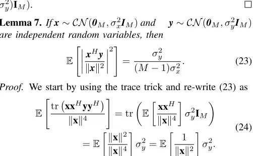
Lemma 7. Ifx∼ CN(0M, σ2xIM)and y∼ CN(0M, σy2IM)
are independent random variables, then
E "
xHy kxk2
2#
= σ
2
y
(M−1)σ2
x
. (23)
Proof. We start by using the trace trick and re-write (23) as
E "
tr xxHyyH kxk4
#
= tr
E
xxH kxk4
σy2IM
=E
kxk2
kxk4
σ2y=E
1
kxk2
σy2.
(24)
A. Proof of the lower-bound with MRC and prop. estimator
Here we show how each one of the terms in (15) are calculated. The term at the numerator is given by
ρE
vHikgiik
2
=ρM2βiik2
E
n
giik+PL
l=1,l6=igilk+wik
oH
giik
kgiik+PL
l=1,l6=igilk+wik
k2
2
,
(25)
which can be found by using Lemma 2 and considering x =giik and y =PL
l=1,l6=igilk+wik
∼ CN(0M,(ζik−
βiik)IM). Therefore, the term in the numerator is found to be
equal to
ρE
vHikgiik
2 =ρM
2β4
iik
ζ2
ik
. (26)
The first term in the denominator can be split into two parts, which are defined as
ρ
L X
l=1
K X
k=1
E|vHikgilk|
2
=ρ
L X
l=1
E|vHikgilk|
2
+ρ
L X
l=1
K X
k0=1,k06=k
E|vHikgilk0|2
. (27)
The first term in the second line of (27) is found by applying Lemma 6 to it, resulting in
ρ L
X
l=1
E|vHikgilk|2
=ρM2β2
iik L
X
l=1 E
n
gilk+PL
l0=1,l06=lgil0k+wik
oH gilk
kgilk+
PL
l0=1,l06=lgil0k+wik
k2
2
=ρM2βiik2 L
X
l=1
(M+ 1)β2
ilk+βilk(ζik−βilk) (M+ 1)ζ2
ik
,
(28) where x =gilk and y =PL
l0=1,l06=lgil0k+wik. The second
term in the second line of (27) is found by applying Lemma 7 to it, where x =zik and y = gilk0. Therefore, the second
term in the second line of (27) is given by
ρ L
X
l=1
K
X
k0=1,k06=k
E|vHikgilk0|2
= ρM
2β2
iik (M−1)ζik
L
X
l=1
K
X
k0=1,k06=k βilk0.
(29) The second term in the denominator is equal to the term in the numerator and therefore does not need to be recomputed.
The third term in the denominator is defined as
Ekvikk2
=M2βiik2 E
1
kzikk2
, (30)
where the expectation in the second part of (30) is found by using Lemma 3 and remembering thatzik∼ CN(0M, ζikIM).
Therefore, the last term is given by
Ekvikk2
= M
2β2
iik
(M −1)ζik
. (31)
Finally, replacing the results found here in (15) concludes the proof.
ACKNOWLEDGMENT
We thank our colleagues from Instituto Eldorado who provided insight and expertise that assisted in this research.
REFERENCES
[1] Cisco, Cisco Visual Networking Index: Global Mobile Data Traffic Forecast Update, 2015-2020, White paper, February 2016.
[2] ITU-R, IMT Vision - Framework and overall objectives of the future development of IMT for 2020 and beyond, September 2015.
[3] Ericsson, Ericsson mobility report, [Online]. Available: http://www.ericsson.com/mobility-report, June 2017.
[4] Van Minh Nguyen, and Marios Kountouris,Performance Limits of Net-work Densification, IEEE Journal on Selected Areas in Communications, vol. 35, no. 6, pp. 1294-1308, June 2017.
[5] Chao Sun, Ling Yang, Li Chen, and Jiliang Zhang,SVR Based Blind Signal Recovery for Convolutive MIMO Systems With High-Order QAM Signals, IEEE Access, vol. 7, pp. 23249-23260, February 2019. [6] Shuanshuan Wu, Rachad Atat, Nicholas Mastronarde, and Lingjia Liu,
Improving the Coverage and Spectral Efficiency of Millimeter-Wave Cellular Networks Using Device-to-Device Relays, IEEE Transactions on Communications, vol. 66, no. 5, pp. 2251-2265, May 2018. [7] Felipe A. P. de Figueiredo, R. Mennes, X. Jiao, W. Liu, and I. Moerman,
A spectrum sharing framework for intelligent next generation wireless networks, IEEE Access, vol. 6, pp. 60704-60735, November 2018. [8] Zhanji Wu, Kun Lu, Chengxin Jiang, and Xuanbo Shao,Comprehensive
Study and Comparison on 5G NOMA Schemes, IEEE Access, vol. 6, pp. 18511-18519, March 2018.
[9] Yuanxue Xin, Dongming Wang, Jiamin Li, Huilin Zhu, Jiangzhou Wang, and Xiaohu You, Area Spectral Efficiency and Area Energy Efficiency of Massive MIMO Cellular Systems, IEEE Transactions on Vehicular Technology, vol. 65, no. 5, pp. 3243-3254, May 2016.
[10] Emil Bjornson, Luca Sanguinetti, Henk Wymeersch, Jakob Hoydis, and Thomas L. Marzetta,Massive MIMO is a Reality - What is Next? Five Promising Research Directions for Antenna Arrays, submitted to Digital Signal Processing, arXiv:1902.07678, February 2019.
[11] S. Kay, Fundamentals of Statistical Signal Processing: Estimation Theory, Prentice-Hall, 1993.
[12] Felipe Augusto P. de Figueiredo et. al.,Channel estimation for massive MIMO TDD systems assuming pilot contamination and flat fading, EURASIP Journal on Wireless Communications and Networking, Jan-uary 2018.
[13] Emil Bjornson, Jakob Hoydis, and Luca Sanguinetti,Massive MIMO Networks: Spectral, Energy, and Hardware Efficiency, Foundations and Trends in Signal Processing: vol. 11, no. 3-4, pp. 154-655, DOI: 10.1561/2000000093, 2017.
[14] T. L. Marzetta,Noncooperative cellular wireless with unlimited numbers of base station antennas, IEEE Trans. Wireless Commun., vol. 9, no. 11, pp. 3590-3600, Nov. 2010.
[15] Thomas L. Marzetta, Erik G. Larsson, Hong Yang, Hien Quoc Ngo, Fundamentals of Massive MIMO, Cambridge U.K., Cambridge Univer-sity Press, 1st edition, November 2016.
[16] T. L. Marzetta,How much training is required for multiuser MIMO?, in Proc. 40th Asilomar Conf. Signals, Syst., Comput. (ACSSC), Pacific Grove, CA, USA, pp. 359-363, Oct. 2006.
[17] G. Caire, N. Jindal, M. Kobayashi, and N. Ravindran,Multiuser MIMO achievable rates with downlink training and channel state feedback, IEEE Trans. Inf. Theory, vol. 56, no. 6, pp. 2845-2866, Jun. 2010. [18] J. Jose, A. Ashikhmin, T. L. Marzetta, and S. Vishwanath, Pilot
contamination and precoding in multi-cell TDD systems, IEEE Trans. Wireless Commun., vol. 10, no. 8, pp. 2640-2651, Aug. 2011. [19] Emil Bjornson, Erik G. Larsson, and Thomas L. Marzetta, Massive
MIMO: ten myths and one critical question, IEEE Commun. Mag., vol. 54, no. 2, Feb. 2016.
[20] Felipe A. P. de Figueiredo, Fabbryccio A. C. M. Cardoso, Ingrid Moer-man, and Gustavo Fraidenraich,Channel Estimation for Massive MIMO TDD Systems Assuming Pilot Contamination and Frequency Selective Fading, IEEE Access, vol. 5, no. 9, pp. 17733-17741, September 2017. [21] George Marsaglia, Ratios of Normal Variables, Journal of Statistical
Software, vol. 16, no. 4, May 2006.