PanORAMa: Oblivious RAM with Logarithmic Overhead
Sarvar Patel∗1, Giuseppe Persiano†1,2, Mariana Raykova‡1,3, and Kevin Yeo§1
1Google LLC 2Universit`a di Salerno
3Yale University
Abstract
We presentPanORAMa, the first Oblivious RAM construction that achieves communication overhead O(logN ·log logN) for database of N blocks and for any block size B = Ω(logN) while requiring client memory of only a constant number of memory blocks. Our scheme can be instantiated in the “balls and bins” model in which Goldreich and Ostrovsky [JACM 96] showed an Ω(logN) lower bound for ORAM communication.
Our construction follows the hierarchical approach to ORAM design and relies on two main building blocks of independent interest: anew oblivious hash table construction with improved amortized O(logN+poly(log logλ)) communication overhead for security parameter λ and
N = poly(λ), assuming its input is randomly shuffled; and a complementary new oblivious random multi-array shuffle construction, which shuffles N blocks of data with communication
O(Nlog logλ+NloglogλN) when the input has a certain level of entropy. We combine these two primitives to improve the shuffle time in our hierarchical ORAM construction by avoiding heavy oblivious shuffles and leveraging entropy remaining in the merged levels from previous shuffles. As a result, the amortized shuffle cost is asymptotically the same as the lookup complexity in our construction.
∗
†
‡
§
1
Introduction
The cryptographic primitive of Oblivious RAM (ORAM) considers the question of how to enable a client to outsource its database to an untrusted server and to query it subsequently without any privacy leakage related to the queries and the database. While encryption can help with hiding the outsourced content, a much more challenging question is how to hide the leakage from the access patterns induced by the queries’ execution. This is leakage that is not only ruled out by the strong formal definition of privacy preserving data outsourcing but has also been proven to be detrimental in many practical outsourcing settings [25, 6]. Hiding access patterns is only interesting when coupled with efficiency guarantees for the query execution in the following sense: there is a trivial access hiding solution which requires linear scan of the whole data at every access. Once such efficiency properties are in place, ORAM constructions also have another extremely important application as they are a critical component for secure computation solutions that achieve sublinear complexity in their input size [31, 24, 40].
Thus, the study of ORAM constructions has been driven by the goal of improving their band-width overhead per access while providing hiding properties for the access patterns. This study has been a main research area in Cryptography for the past thirty years, since the notion was introduced by Goldreich [18], and it has turned ORAM into one of the classical cryptographic concepts. The seminal works of Goldreich and Ostrovsky [18, 30, 19] introduced the first ORAM constructions achieving square root and polylogarithmic amortized query efficiency. These early works also considered the question of a lower bound on the amortized communication complex-ity required to maintain obliviousness. They presented a lower bound result of O(logCN) blocks of bandwidth overhead for any ORAM construction for a database of size N blocks and a client with memory that can store C blocks. However, this result came with a few caveats, which were clarified and more carefully analyzed in the recent work by Boyle and Naor [5]. A recent work of Larsen and Nielsen [27] removed these caveats in the online model and presented an Ω(logN) block communication lower bound for general storage models and computationally bounded adversaries.
ORAM Communication Lower Bound. The ORAM communication lower bound presented by Goldreich and Ostrovsky [19] applied to constructions using restricted manipulation on the underlying data (i.e., treating the data as monolithic blocks that are read from, written to and moved between different memory positions), achieving statistical security and any block size. Boyle and Naor [5] formalized the model of this lower bound as the “balls and bins” storage model and gave much more insight into understanding the lower bound of Goldreich and Ostrovsky. They provided evidence that extending the lower bound beyond the restricted model in the original result will be a challenging task by showing a reduction from sorting circuits to offline ORAM where all queries are given ahead of time, which essentially means that extending the offline ORAM lower bound will imply new lower bounds for sorting circuits. At the same time, Boyle and Naor introduced an online model for ORAM where queries are selected adaptively during execution. This model avoids the relation to the lower bound on sorting circuits while reflecting the functionality of most existing ORAM constructions, which opened the possibility that improving the lower bound in the online model might be easier than in the offline setting. The recent work of Larsen and Nielsen [27] proved the best ORAM lower bound which applies to the online model with computational guarantees, and for any general storage model. However, the server is assumed to act only as storage and it is known that allowing server-side computation can bypass the lower bound [14].
size. While there are constructions [38, 40] that match the lower bound in regimes when they are instantiated with appropriately big block sizes, there is no known result that meets the lower bound for every block size Ω(logN).
ORAM Constructions. While the lower bound of Goldreich and Ostrovsky has its caveats, it has become the measure to compare with for every new construction with improved complexity. We next overview the known ORAM constructions, their models and efficiency with respect to the requirements for the lower bound. Existing ORAM schemes could be roughly divided into two categories: constructions [35, 1, 13, 22, 26] that follow the hierarchical blueprint introduced in the work of Goldreich and Ostrovsky [30, 19], and constructions [37, 17, 38, 12, 40, 36, 7] that follow the tree-based template with a recursive position map, which was introduced in the work of Shi et al. [37].
The idea underlying the first class of constructions is to divide the data in levels of increasing size that form a hierarchy and to instantiate each level with an oblivious access structure that allows each item to be accessed obliviously only once in that level. The smallest level in the hierarchy is linearly scanned at each access and each block that is accessed is subsequently moved to this level. To prevent overflowing of the top levels, there is a deterministic schedule, independent of the actual accesses, that prescribes how blocks move from the smaller to the bigger levels.
Within the general hierarchical framework, the main optimization question considered in differ-ent constructions is how to instantiate the oblivious structure in each level. The original Goldreich-Ostrovsky construction [19] used pseudorandom functions (PRFs) resulting inO(log3N) amortized communication overhead. Later, the work of Pinkas and Reinman [35] proposed the use of Cuckoo hash tables. This work suffered from a subtle issue related to the obliviousness of the Cuckoo hash tables, which was later fixed in the work of Goodrich and Mitzenmacher [22] who showed an ele-gant algorithm to obliviously construct a Cuckoo hash table. Their main argument was a reduction of the Cuckoo hash table construction to oblivious sorting that resulted in a O(log2N)-overhead ORAM. Subsequently, Kushilevitz et al. [26] devised a balancing scheme that further improved the bandwidth toO(log2N/log logN). The work of Chan et al. [7] presented a unified framework for hierarchical ORAM constructions and made explicit the notion of an oblivious hash table in order to capture the properties of the oblivious structure needed for each level. All the above constructions require that the client’s memory can hold only a constant number of blocks.
The known hierarchical ORAM constructions do not make any assumptions about the block sizes used to store data in memory and can be instantiated with any block size B = Ω(logN). Even the construction with best asymptotic efficiency among existing schemes, when instantiated with a private random function in the balls and bins model, does not meet the logarithmic lower bound in the case of client’s memory that holds only a constant number of blocks.
to the concrete eviction algorithms they use, which have been evolving and improving the ORAM access overhead. The work of Shi et al. [37] that pioneered the tree-based approach achieved
O(log3N) communication. Gentry et al. [17] improved the overhead to O(log loglog3NN). Currently the most efficient tree-based construction is the Path ORAM construction [38], which achieves
O(log2N) bandwidth overhead for general block sizes. If instantiated with blocks of size Ω(log2N), Path ORAM has bandwidth overhead of O(logN) blocks. The same efficiency holds for Circuit ORAM [40], which optimizes circuit sizes for ORAM access functionality in secure computation.
The only computational assumption of the above tree-based constructions is related to the encryption used to hide the content and thus they do offer statistical guarantees in the balls and bins model. Several works [14, 28] also demonstrate how to bypass the lower bound of communication complexity, if the server is allowed to do computation on the data it stores, which is enabled by homomorphic encryption.
Our Contributions. In this paper we present PanORAMa, a computationally secure oblivious RAM withO(logN·log logN) bandwidth overhead and constant client memory1. Our construction works for any block size B = Ω(logN). This assumption is very natural since all known ORAM constructions including ours require that the blocks store their own addresses for correctness and this already takes Θ(logN) bits. In addition,PanORAMais in the balls and bins model of Boyle and Naor [5] as it treats each data block as an atomic piece of data and the server only fetches blocks from memory, writes blocks to memory and moves blocks between different memory positions. Thus,
PanORAMa achieves currently the best asymptotic communication overhead among constructions that work with general block sizes, operate in the balls and bins model and require constant number of blocks client memory.
Our construction can be modified in a straightforward way to obtain statistical security in the balls and bins model if the client is provided with access to a private random function, which matches the assumptions in the original lower bound (see Theorem 6 in [19]). In this case, we obtain a balls and bins construction that is onlyO(log logN) away from the lower bound overhead proven by Goldreich and Ostrovsky [19]. Our construction is alsoO(log logN) away from the lower bound by Larsen and Nielsen [27] for general storage models and computational adversaries. As a result, we show that the balls and bins model of computation is almost as strong as any general storage model and can only require at mostO(log logN) extra communication overhead.
The PanORAMa construction relies on two main building blocks, which can have applications outside ORAM of independent interest: an oblivious hash table (OHT) and an oblivious random multi-array shuffle algorithm. For both, we provide new efficient constructions. Specifically,
• Oblivious Hash Table (OHT). An oblivious hash table offers the same functionalities as a regular hash table (efficient storage and access) while guaranteeing access obliviousness for non-repeating patterns. We extend the definition of OHT [7] that consists of initialization and query algorithms as follows. We split the initialization into Init, which shuffles the input items and inserts dummies, andBuild, which uses the output ofInitto create the OHT storage structure. We add an algorithm Extract, which obliviously returns all unqueried items from the OHT appropriately padded. Our OHT construction offers an amortized access efficiency ofO(logN+ log logλ) blocks assuming the starting data is randomly shuffled, whereλis the security parameter.
1
• Oblivious Random Multi-Array Shuffle. Complementary to the OHT primitive is our efficient oblivious random multi-array shuffle algorithm that shuffles together data which initial order has partial entropy with respect to the adversary. More precisely, our algorithm shuffles together A1, . . . , AL arrays of total size N, each of which is independently and randomly
shuffled. Suppose that theLarrays are arranged in decreasing size. Then, our shuffle requires
O(Nlog logλ+NloglogλN) blocks of communication when there existscutoff =O(log logλ) such that|Acutoff|+. . .+|AL|=O(Nlog loglogN λ).
Technical Overview of Our Result. Our ORAM construction follows the general paradigm of hierarchical ORAM constructions as laid out by Goldreich and Ostrovsky [19] (see Chan et al. [7] for a formalized presentation of the framework). As we discussed above, the hierarchical constructions distribute the data in several levels, which are instantiated with oblivious hash tables that provide access obliviousness for non-repeating queries.
In order to prevent overflow of the OHTs implementing the ORAM levels, every 2i accesses, all levels of size less or equal than 2i are merged and shuffled together and placed in an oblivious data structure in the level of capacity 2i+1. While a level of capacity 2j ≤ 2i services exactly 2j queries before shuffling, the number of real items retrieved from this level can range from 0 to 2j. All queried items have been moved to smaller levels and thus should not be included in the shuffle as items coming from this level. The remaining at most 2j unqueried items in the oblivious data structure need to be extracted and included in the larger capacity level for future queries. As a result, the shuffle step can be broken down into three phases: extracting unqueried items from each level, merging the content of multiple levels and initializing a oblivious hash table for the new level. For many existing hierarchical ORAMs, the dominant cost in the communication complexity arises from to the use of several oblivious sorts that are used to implement the shuffling functionality while removing queried items. The best known data-oblivious sorting algorithms [39, 20, 21, 8] used in these constructions require communicationO(NlogN). In our work, we show that all three shuffle phases can be achieved without the use of expensive oblivious sorts by leveraging and maintaining entropy from previous shuffles, which is manifested in the fact that the unqueried items in each level are essentially “randomly shuffled”. Similar ideas were previously explored for simpler scenarios in [34].
is exactly the distribution we need for the new level that will be initialized after the shuffle. We discuss the intuition for efficient extraction in the overview of our OHT construction in Section 4. The next step of the shuffle is to obliviously merge all extracted items from multiple levels. One way to achieve this is using an oblivious sort over all items, which would require O(NlogN) for the largest levels. Oblivious sorting achieves very strong hiding guarantees even against an adversary that knows the entire initial order of the data. However, in the case of the ORAM shuffle mixing together the items from the shuffled ORAM levels, we have the additional leverage that the inputs for the shuffle coming from the extraction of each OHT at each level are already randomly shuffled arrays. More specifically these are multiple arrays of geometrically decreasing size where each array is randomly ordered in a manner oblivious to the adversary. We design an oblivious random multi-array shuffle that obliviously merges the randomly ordered input arrays into a single array, which is a random shuffle of all elements. This algorithm leverages the entropy coming from the random shuffles of each input array to avoid the cost of expensive oblivious sort. We discuss the intuition behind this algorithm in the overview our multi-array shuffle in Section 3.
The final phase in the ORAM step shuffle is the OHT initialization for level i+ 1 using the randomly permuted array that is output from the multi-array shuffle. We manage to construct an efficient algorithm for the initialization that avoids oblivious shuffles of the whole input by crucially relying on the fact that the input is already randomly shuffled. We further discuss the intuition for the initialization algorithm of our OHT construction in Section 4.
Oblivious Hash Table. Our oblivious hash table construction is inspired by the two-tier hash scheme proposed by Chan et al. [9], however, with some significant changes that enable constructing the OHT without using an oblivious sort on all the data blocks. The idea of Chan et al. [9] is to allocate the database items into bins on the first level of the hash table using a PRF, where the size of the bins is set to be O(logδλ), for some constant 0 ≤ δ < 1, which does not guarantee non-negligible overflow probability. All overflow items are allocated to a second level where they are distributed using a second PRF. In order to initialize this two-tier hash scheme, the authors use an oblivious sort which comes at a costO(NlogN) for N blocks of data.
Our goal is to obtain a construction of an oblivious hash table that allows more efficient oblivious initialization assuming that the database items are already randomly shuffled. The assumption of the randomly shuffled input is not arbitrary. We will use our oblivious random multi-array shuffle to construct this random shuffle of the input in the context of our ORAM construction.
Our initialization algorithm sequentially distributes input items in O(log logλ) levels. At each level, all remaining items are distributed into small bins according to a secret PRF where the bin sizes are not hidden. A secret distribution for each bin’s real size is sampled and several small oblivious shuffles are employed to remove additional blocks from each bin for the next level. In more detail, we first assign items into buckets according to a PRF non-obliviously taking linear time in the size of the data. Then, we sample from a binomial distribution loads for all bins that correspond to randomly distributing only fraction of the total number of items. We choose a cutoff point,thrsh, such that with overwhelming probability, it is larger than any bin load sampled from the binomial distribution in the second step and, at the same time, is smaller than any load from the distribution of items induced by the PRF in the first step. We cut the size of each bin to exactly thrsh items, among which there will be as many real items as the loads sampled from the binomial distribution and the rest will be dummy items. The remaining overflow items are distributed recursively in following levels of the OHT where the size of the smallest level is
they will be distributed according to the bin loads induced from the binomial samples, which are independent from the loads due to the PRF that the server observed in the clear.
The items assigned to each bin in each level of the OHT are instantiated with another oblivious hash table construction which we call oblivious bin. An oblivious bin is an OHT with small input sizeO(poly(logλ)) for which we can afford to use an oblivious sort for initialization and extraction without incurring prohibitive efficiency cost. In the full version [32] we present an instantiation for oblivious bins using a Cuckoo hash table.
The OHT query algorithm consists of one oblivious bin query in each level. The single bin in the smallest level is always queried. In every other level, we either query the bin determined by the corresponding PRF if the item has not been found yet, or query a random bin otherwise.
Last but not least, our oblivious hash tables have an oblivious extraction procedure that allows to separate the unqueried items in the OHT with just an overhead ofO(log logλ) per item. Addi-tionally we guarantee that the extracted items are randomly shuffled and, thus, we can use them directly as input for our multi-array shuffle. The extraction procedure for our OHT can be done by implementing the extraction on each of the oblivious bins and concatenating the outputs, since the items were distributed to bins using a secret distribution function. We obliviously extract each bin using an oblivious sort.
Oblivious Random Multi-Array Shuffle. Our multi-array random shuffle relies on the obser-vation that we do not need to hide the access pattern within each of the input arrays since they are already shuffled. Recall that in the context of ORAM, these input arrays represent the unqueried items extracted from OHTs of smaller levels. Since our shuffle algorithm will be accessing each entry of each input array only once, its initial random shuffle suffices for the obliviousness of these accesses. However, the multi-array shuffle algorithm still needs to hide the interleaving accesses to the different input arrays. One way to achieve this is to obliviously shuffle the accesses to different input arrays. If we do this, in general, we will end up doing an oblivious shuffle on the whole input data, which is too expensive.
Instead, we partition the input arrays by distributing their items at random into a number of bins of size O(log1−32λ). We also partition the output array into bins of size O(log3λ), where each item of the output array is assigned an input array tag that is encrypted and remains hidden. With all but negligible probability each resulting input bin contains a sufficient number of items from each input array in order to initialize each output bin. The partitioning into input and output bins is performed non-obliviously but does not cause any additional leakage as the inputs arrays are shuffled and the input arrays tags for all output array items are encrypted.
We pair input and output bins and we use items from an input bin to initialize the items in the corresponding output bin using a sequence of oblivious sorts. In each such initialization, we also have a number of leftover real items that were not needed for the output bin (the sizes of the input and output bins were chosen in a way that guarantees that we always have at least as many items from each input array in the input bin as needed in the output segment). We apply the multi-array random shuffling algorithm recursively on the arrays containing leftover items from the executions filling different output bins in order to initialize the remaining output bins (there were more output bins than input bins but output bins had smaller sizes). After all items have been distributed from input bins to output bins using the above construction, we use to reverse mapping from output bins to the output array to place the items in the output array.
Thus, the total shuffle cost remains O(Nlog logλ).
Our resulting shuffling procedure achieves such efficiency that it is no longer the dominant cost in the amortized query complexity for our final ORAM construction. As a result, the optimization technique presented in the work of Kushilevitz et al. [26], which balances the cost of the lookups and the cost of the shuffle by splitting each level into several disjoint oblivious hash tables that get shuffled into separately, does not result in any efficiency improvement when applied to our scheme.
Paper Organization. We present in Section 2 the definitions of the primitives we use in the rest of the paper. Section 3 describes our construction of an oblivious random multi-array shuffle, which relies on permutation decomposition lemmas that provide alternative ways to sample randomly a permutation, which are presented in Appendix A. In Section 4 we describe our general oblivious hash table construction and its building block the oblivious bin primitive. Finally, we present our ORAM construction in Section 5. In Appendix B we present an additional overview of related work.
2
Definitions
In this section we present the definitions for the existing primitives that we use for our constructions as well as definitions of the new primitives that we introduce in our work.
Notation. We denote Binomial[n, p] the binomial distribution with parameters: n trials each of which with success probability p. We use X ← Binomial[n, p] to denote that the variable X is sampled from the binomial distribution according to its probability mass function Pr(k;n, p) =
Pr[X = k] = nkpk(1−p)n−k. In a setting where an algorithm Alg is executing using external memory, we denote byAddrs[Alg] the memory access pattern that consists of all accessed addresses in the memory. We use PPT as a shorthand for “probabilistic polynomial-time.”
In analyzing our constructions, we express bandwidth and client memory using the size B of a block as a unit.
2.1 Oblivious RAM
Definition 1 (Oblivious RAM). An oblivious RAM scheme ORAM= (ORAM.Init,ORAM.Access) consists the following two algorithms:
• ( ˜D,st) ← ORAM.Init(1λ, D): the initialization algorithm takes as input a database D and outputs a initialized memory structure ˜D.
• (v,st0) ← ORAM.Access(st,D,˜ I): the ORAM access algorithm takes as input the ORAM database ˜D, the current state st as well as an instruction I = (op,addr,data), where op ∈ {read,write} and if op=read, then data= ⊥. If op= read, the access algorithm returns as
v the data stored at address addr in the database. Else, if op =write the access algorithm writesdata in locationaddr in the database. Furthermore, an updated statest0 is returned. The resulting construction is oblivious if there exists a PPT simulator Sim= (SimInit,SimAccess)
such that for any PPT adversarial algorithmA and for any n=poly(λ),
Pr
h
b= 1 |b←ExptAReal,ORAM(λ, n)i−Prhb0 = 1 |b0 ←ExptSimIdeal,A,ORAM(λ, n)i
<negl(λ),
ExptAReal,ORAM(λ, n) ExptSimIdeal,,AORAM(λ, n)
(D,stA)← A1(1λ) (D,stA)← A1(1λ)
χ←Addrs[( ˜D,st)←ORAM.Init(1λ, D)] χ←Addrs[( ˜D,stSim)←SimInit(1λ,|D|)]
forj = 1 ton fori= 1 ton
(Ij,stA)← A2(stA,D, χ˜ ) (Ij,stA)← A2(stA,D, χ˜ )
χAccess←Addrs[(st,D˜)←ORAM.Access(st,D,˜ Ij)] χAccess←Addrs[(st,D˜)←SimAccess(stSim)]
χ←χ∪χAccess χ←χ∪χAccess
2.2 Oblivious Random Multi-Array Shuffle
In oblivious shuffling, we have one array ofN data blocks and the task of the algorithm is to shuffle the blocks into a destination array so that an adversary observing the accesses of the algorithm to the blocks does not obtain any information regarding the final permutation. The security guarantee holds even if the initial arrangement of the blocks is known to the adversary. This is sufficient to be used in the design of Oblivious RAM. An oblivious random multi-array shuffle instead offers a weaker security guarantee, which we show also suffices for the design of an Oblivious RAM. For a range of parameters of interest, we present an implementation with improved efficiency in terms of bandwidth overhead compared to oblivious shuffling. Roughly speaking, in an oblivious random multi-array random shuffle, we have N blocks partitioned into L arrays A1, . . . ,AL and
the task is to shuffle the N blocks into a destination array according to a permutation chosen uniformly at random. The associated security notion still guarantees that no information regarding the final permutation of the blocks is leaked. However, the adversary’s knowledge is limited to the distribution of blocks to each array and does not include each block’s specific location within the array. Let us now proceed more formally.
2.3 Oblivious Bin
We introduce a slight modification of our oblivious hash table definition, which we call oblivious bin. As the name implies, we will use this oblivious structure to store and access data in oblivious manner within bins which will be used as building blocks in out oblivious hash table scheme. We will use the oblivious bin for data of smaller size.
Definition 2(Oblivious Bin). An oblivious hash table schemeOblivBin= (OblivBin.Init,OblivBin.Build,
OblivBin.Lookup,OblivBin.Extract) consists of the following algorithm:
• ( ˜D,st) ← OblivBin.Init(D): an algorithm that takes as input an array of key-value pairs
D={(ki, vi)}N
i=1 and outputs a processed version of it ˜D.
• ( ˜S,H,˜ st0)←OblivBin.Build( ˜D,st): an algorithm that takes as input a processed database ˜D
and a state and initializes the hash table ˜H and an additional array ˜S and updates the state
st.
• (v,S˜0,H˜0,st0) ←OblivBin.Lookup(k,H,˜ S,˜ st): an algorithm that takes as input the oblivious hash table, the additional array, the state produced in the build stage and a lookup key, and outputs the value vi corresponding to the key ki together with updated hash table ˜H0 and
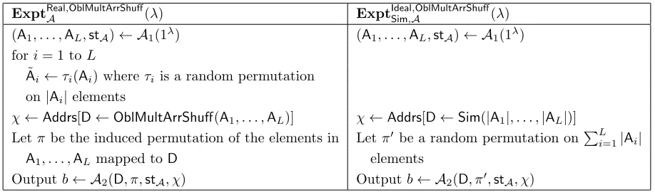
ExptAReal,OblMultArrShuff(λ) ExptSimIdeal,,AOblMultArrShuff(λ)
(A1, . . . ,AL,stA)← A1(1λ) (A1, . . . ,AL,stA)← A1(1λ)
fori= 1 toL
˜
Ai ←τi(Ai) whereτi is a random permutation
on|Ai|elements
χ←Addrs[D←OblMultArrShuff(A1, . . . ,AL)] χ←Addrs[D←Sim(|A1|, . . . ,|AL|)]
Letπbe the induced permutation of the elements in Letπ0 be a random permutation onPL
i=1|Ai|
A1, . . . ,AL mapped toD elements
Outputb← A2(D, π,stA, χ) Outputb← A2(D, π0,stA, χ)
Figure 1: Real and ideal executions for OblMultArrShuff.
• ( ˜D,st0) ← OblivBin.Extract( ˜H,S,˜ st): this is an algorithm that takes the hash table, the auxiliary array and the state after the execution of a number of queries and outputs a database, which contains only the unqueried items (ki, vi)∈D and is padded to sizeN.
The oblivious property for a bin is identical to that of the oblivious hash table.
2.4 Oblivious Random Multi-Array Shuffle
We start with the definition of a random multi-array shuffling algorithm that obliviously shuffles together the content of several input array each of which is independently shuffled (see full version for more detailed discussion of the functionality).
Definition 3(Oblivious Random Multi-Array Shuffle). Arandom multi-array shufflealgorithm is an algorithmD←OblMultArrShuff(A1, . . . ,AL) that takes as input LarraysA1, . . . ,AL containing
a total of N blocks and outputs a destination array D that contain all N blocks. Each of the L
arrays are assumed to have been arranged according to a permutation chosen uniformly at random. The blocks inD should be arranged according to a permutation chosen uniformly at random.
A random multi-array shuffle algorithm OblMultArrShuff is oblivious if there exists a PPT simulator Sim, which takes as input (|A1|, . . . ,|AL|), such that for any PPT adversary algorithm
A= (A1,A2):
Pr
h
b= 1 |b←ExptRealA ,OblMultArrShuff(λ)i−Prhb0 = 1|b0 ←ExptIdealSim,A,OblMultArrShuff(λ)i<negl(λ)
where the real and ideal executions are defined in Figure 1.
2.5 Oblivious Hash Table
Next we define our oblivious hash table, which provides oblivious access for non-repeating queries. In addition, it has an extraction algorithm which allows to extract obliviously the unqueried items remaining in the OHT in a randomly permuted order.
Definition 4 (Oblivious Hash Table). An oblivious hash table scheme OblivHT = (OblivHT.Init,
OblivHT.Build,OblivHT.Lookup,OblivHT.Extract) consists of the following algorithms:
• ( ˜D,st) ← OblivHT.Init(D): an algorithm that takes as input an array of key-value pairs
D={(ki, vi)}N
i=1 and outputs a processed version of D, which we denote ˜D.
• ( ˜H,st0) ← OblivHT.Build( ˜D,st): an algorithm that takes as input a processed database ˜D
and a state and initializes the hash table ˜H and updates the statest.
• (v,H˜0,st0) ←OblivHT.Lookup(k,H,˜ st): an algorithm that takes as input the oblivious hash table, ˜H, the state produced in the build stage,st, and a lookup key,k, and outputs the value
vi corresponding to the key ki together with an updated hash table, ˜H0, and updated state,
st0. If the kis a dummy query, thenv:=⊥.
• ( ˜D,st0) ←OblivHT.Extract( ˜H,st): an algorithm that takes the hash table, ˜H, and the state after the execution of a number of queries,st, and outputs a database ˜D, which contains only the unqueried items (ki, vi)∈Dand is padded to sizeN with dummy items, and the content
of ˜Dis randomly permuted.
The resulting hash scheme is oblivious if there exists a PPT simulator Sim= (SimInit,SimBuild,
SimLookup, SimExtract), which takes as input the size of the database |D|, such that for any PPT
adversary algorithm A= (A1,A2,A3) and for any n=poly(λ),
Pr
h
b= 1 |b←ExptRealA ,OblivHT(λ, n)
i
−Pr
h
b0 = 1 |b0←ExptIdealSim,A,OblivHT(λ, n)
i
<negl(λ),
where the real and ideal executions are defined in Figure 2.
Although it may not be apparent at this stage why we have separateOblivHT.InitandOblivHT.Build
algorithms, the reason is that in the context of our ORAM construction we will instantiate the
OblivHT.Initalgorithm with our oblivious random multi-array shuffle.
We want to guarantee that the output ofExtractalgorithm is randomly shuffled from the point of view of the adversary. We formalize this similarly to the oblivious random multi-array shuffle, by providing the adversary with the real induced permutation in the real execution and a random independent permutation in the ideal execution. If the adversary cannot distinguish which is the real permutation, it means that it did not learn anything from the access patterns it observed.
3
Oblivious Random Multi-Array Shuffle
ExptAReal,OblivHT(λ, n) ExptSimIdeal,,AOblivHT(λ, n)
(D,stA)← A1(1λ) (D,stA)← A1(1λ)
χInit ←Addrs[( ˜D,st)←OblivHT.Init(D)] χInit ←Addrs[( ˜D,stSim)←SimInit(|D|)]
χBuild←Addrs[( ˜H,st)←OblivHT.Build(D,st)] χBuild ←Addrs[( ˜H,stSim)←SimBuild(|D|)]
χLookup ←⊥,χ←(χInit, χBuild) χLookup ←⊥,χ←(χInit, χBuild)
fori= 1 ton fori= 1 ton
(ki,stA | {ki6=kj}1≤j<i)← A2( ˜H,stA, χ, χLookup) (ki,stA | {ki6=kj}1≤j<i)← A2( ˜H,stA, χ, χLookup)
χLookup ←Addrs[( ˜H, vi,st)←OblivHT.Lookup(ki,H,˜ st)] χLookup ←Addrs[( ˜H,stSim)←SimLookup( ˜H,stSim)]
χExtract←Addrs[( ˜D,st)←OblivHT.Extract( ˜H,st)] χExtract←Addrs[ ˜H ←SimExtract( ˜H,stSim)]
Letπbe the permutation induced on the itemsD\ {ki}ni=1 Letπ0 be a random permutation onN items
and the padding dummies in ˜D
Outputb← A3( ˜D, π,stA, χExtract) Outputb← A3( ˜D, π0,stA, χExtract)
Figure 2: Real and ideal executions for OblivHT.
achieving bandwidth ofO(Nlog logλ+NloglogλN) blocks forN data blocks. Our entropy requirement for the input comes in the following form: the N input blocks are divided in L input arrays,
A1, . . . ,AL, each of which is randomly permuted in a manner unknown to the server storing the
arrays. The arrays have sizes N1, . . . , NL where Ni ≥ Ni+1 for i = 1, . . . , L, and there exists
cutoff = O(log logλ) such that |Acutoff|+. . .+|AL| = O(Nlog loglogN λ) and |Ai| = Ω(logNλ) for all i∈ {1, . . . ,cutoff−1}, which is the case for geometrically decreasing input array sizes that arise in the context of the ORAM shuffles.
As all the input arrays are randomly ordered, it suffices to distribute items based only on the array indices. To ensure the expectations are tightly concentrated, we require input arrays to be at least Ω(logNλ) size. Thus, as a first step all small input arrays must be shuffled together in a single input array using an oblivious sort. Next we randomly sample an assignment,Assign, that specifies an array index,i∈[L] for each location of the output arrayDwith the intention that ifAssign(j) =i
for some output array index,j∈[N], then our algorithm should distribute an item from input array
Ai to the j-th location of the output array, D[j]. To distribute items, our algorithm randomly
partitions each of the input arraysA1, . . . ,ALinto ˜minput bins,Binin1, . . . ,Bininm˜, of expected polylog
size, i.e., each input bin contains elements from all input arrays. The output array D is also partitioned intomoutput bins,Binout1 , . . . ,Binoutm , of expected polylog size but slightly smaller than the input bins Binin. To ensure output bins are smaller, m is chosen to be larger than ˜m. We pair up input bins and output bins until we run out of output bins. As long as the input arrays are large enough, it can be shown that any input bin will have sufficient number of blocks from each input arrays to fill in the output array locations of the corresponding output bin according to
Assign. Using oblivious sorts on both the input and output bin, the blocks in the input bin can be obliviously placed into the corresponding output array locations. All unused blocks of the input bin are padded to hide sizes and placed back into leftover bins LeftoverBin which are separated according to their original input arrays.
bins are initialized in the recursive steps does not have any additional leakage as long as we are hiding which items from each input array are placed in these output bins. This is achieved by the oblivious manner of initializing the leftover bins. Each iteration reduces the input items by a constant fraction. AfterO(log logN) recursive iterations, there are O(logNN) remaining items, and we use an oblivious sort to complete the algorithm with only O(N) overhead.
Construction 5. [Oblivious Random Multi-Array Shuffle] We define our oblivious random multi-array shuffle algorithmOblMultArrShuff, which will also use algorithms OblMultArrShuff.BinShuffle
and OblMultArrShuff.Shuffleas building blocks.
OblMultArrShuff. This algorithm takes as input L shuffled arrays and outputs array D, which contains a random permutation of the input array elements.
D←OblMultArrShuff(A1, . . . ,AL):
1. Initialize the output arrayD to be an empty array of sizeN :=|A1|+. . .+|AL|blocks.
2. Choose the largestcutoff such that|Acutoff| ≥ logNλ and then randomly permute the entries of
the arraysAcutoff, . . . ,AL intoA0,cutoff using an oblivious random shuffle.
3. Initialize A0,1, . . . ,A0,cutoff−1 with the content ofA1, . . . ,Acutoff−1 respectively.
4. Sample a random assignment functionAssign: [N]→[cutoff] such that|{b∈[N] :Assign(b) =
i}|= |A0,i| for every i∈ [cutoff]. Since we assume only constant local memory, which does
not fit the description ofAssign, we use the following oblivious algorithm for samplingAssign
at random:
(a) Store an encryption ofcnti:=|A0,i|, fori∈[cutoff] and an encryption ofcnt=N on the
server.
(b) For each block b∈ [N], setAssign(b) = iwith probability cnti
cnt, for i∈ [cutoff]. We do
this obliviously as follows: choose a random value rb ∈ [cnt] and set Assign(b) to be
equal to the minimals such that cnt1+. . .+cnts ≥rb and sis computed by scanning
the encrypted integers cnt1, . . . ,cntcutoff. During the scanning cnts and cnt are each
decreased by 1. Store (b,Enc(Assign(b)) at the server.
5. Let E0 be the array{(b,Enc(Assign(b)))}b∈[N] describing Assign computed and stored at the
server in the previous step. Note, the server knows the first indices of each pair inE0 as they
are unencrypted.
6. SetL:=cutoff.
7. Run OblMultArrShuff.Shuffle(A0,1, . . . ,A0,L,D,E0, N,0).
8. Return D.
OblMultArrShuff.Shuffle.This algorithm takes as inputLrandomly shuffled arrays, an output array
D, which might be partially filled, the set of empty indicesbiinDtogether with their corresponding
encryptedAssign(bi) values stored inE`, and an index`corresponding the current level of recursion.
The algorithm fillsDthrough several recursive steps using the encrypted values ofAssigninE` and
the input arraysA`,1, . . . ,A`,L.
1. If|A`,1|+. . .+|A`,L| ≤ logNλ, assign the items inA`,1, . . . ,A`,Lto the remaining open positions
inDusing theAssign mappings stored inE` by running:
OblMultArrShuff.BinShuffle(A`,1∪. . .∪A`,L,E`,D).
2. Setm:= (2)`logN3λ and ˜m:= (1−2)m.
3. Initialize ˜m input binsBinin1 , . . . ,Bininm˜ with random subsets of blocks from the inputs arrays as follows. For each input array A`,i, i ∈ [L] distribute its blocks across Binin1, . . . ,Bininm˜
assigning each block a bin at random and recording an encryption of the source array index
i. The items ofBinin1 , . . . ,Bininm˜ are stored encrypted on the server. Note Binin1, . . . ,Bininm˜ will have different sizes. Furthermore, the above is done in a non-oblivious manner and the server knows the distribution of the blocks from eachA`,i across the input bins.
4. Initialize moutput binsBinout1 , . . . ,Binoutm with random subsets of pairs from E` by assigning
each pair from E` to a randomly selected bin. The items of Binout1 , . . . ,Binoutm are stored
encrypted on the server. Note the sizes of Binout1 , . . . ,Binoutm will be different. Furthermore, the above is done in a non-oblivious manner and the server knows the distribution of the blocks from eachE` across the output bins. Therefore, the server knows the subset of positions from
Dassigned to each output bin - these are the bvalues in each pair (b,Enc(Assign(b))) ofE`.
5. Initialize A`+1,1, . . . ,A`+1,L to be empty block arrays.
6. Forj= 1, . . . ,m˜:
(a) Distribute the blocks from Bininj in D according to the positions specified by Assign in the pairs inBinoutj by running
(LeftoverBin1, . . . ,LeftoverBinL)←
OblMultArrShuff.BinShuffle(Bininj ,Binoutj ,D).
(b) Append LeftoverBini toA`+1,i for alli∈[L].
7. Collect all uninitialized indices inDtogether with their corresponding mappings underAssign, which have been distributed in output binsBinoutm˜+1, . . . ,Binoutm , and setE`+1 :=Binoutm˜+1∪. . .∪
Binoutm .
8. Execute recursively the shuffling functionality on the remainders of the input arrays, which have not been placed inDso far but were returned as leftovers from theOblMultArrShuff.BinShuffle
executions above, by runningOblMultArrShuff.Shuffle( A`+1,1, . . . ,A`+1,L,D,E`+1, `+ 1).
BinShuffle. This is an algorithm that takes as input a binBininthat contains items, a binBinoutthat contains mappings underAssign of a subset of indices in the inputD. BinShuffledistributes all but an 2fraction of the items inBinin intoDaccording to the mappings and positions ofDspecified in
Binout. The items ofBininthat are not placed inDare returned in leftover bins separated according to their input arrays.
1. Fori∈[L], create NumLeftoveri := (4)NNilog3λdummy blocks tagged with an array index i
and append them encrypted toBinin.
2. Obliviously sortBininaccording to array index of the blocks placing real blocks before dummy blocks with the same array index.
3. Letkouti be the number of pairs (b,Assign(b))∈Binout such that Assign(b) =ifor all i∈[L]. We compute the valueskouti privately in the following oblivious manner:
(a) Initialize allkout
1 , . . . , kLout to 0 and store them encrypted on the server.
(b) For each pair (b,Assign(b)) ∈ Binout, scan all the ciphertexts of kout1 , . . . , kLout and only increment kAssignout (b).
4. Tag all items inBinin withmoving, if they are a real item that will be placed in Dusing the
Assignmapping fromBinout;leftoverif they are real or dummy items that will be returned as leftover; or unusedif they are dummy items that will be discarded. We obliviously tag items as follows: for each blockj inBinin:
(a) Letibe the input array index of the j-th block inBinin.
(b) Fort∈[L], download the counterkoutt . Ift6=i, reencrypt and upload back the counter. Ift=i, upload an encryption of a decremented counterEnc(koutt −1).
(c) Tag the j-th block as follows: if k`,iout > 0, then the block is marked as real. If
−NumLeftoveri< kout`,i ≤0, then the block is marked as leftover. Otherwise, the block is
marked asunused.
5. Obliviously sortBininaccording to the tags computed in the previous step in a manner where all blocks with tag moving precede all blocks with tag leftover and both of these precede blocks with tags unused. All blocks with the same tag are sorted according to their input array index.
6. The blocks inBininare separated in the following way:
(a) Blocks that will be placed in D - these are the first |Binout| blocks in the sorted Binin, which are moved toTempD;
(b) Blocks that will be returned as leftover blocks: these are the next Lgroups of blocks of sizesNumLeftover1, . . . ,NumLeftoverLblocks, which are placed inLeftoverBin1, . . . ,LeftoverBinL
respectively.
7. Obliviously sort the pairs (b,Assign(b)) in Binout according to input array index Assign(b). Before sorting, encrypt theb value of each pair of Binout to ensure obliviousness. Recall the
Assign(b) value is already encrypted. Note that TempD and Binout now contain the same numbers of items tagged with each of the input array indices, which are also sorted according to these indices. Thus, for each position i∈[|Binout|], the block in position iin TempD has input array index equal toAssign(bi), where (bi,Assign(bi)) is thei-th pair in the sortedBinout.
8. Assign to each block in TempD its corresponding location in D as follows: fori∈ [|Binout|], tag the block in positioniinTempDwith an encryption ofbi, where (bi,Assign(bi)) is thei-th
9. Obliviously sortTempDaccording to tags computed in the previous step and copy the content of TempD in the positions denoted by their tags inD. Note these positions of D are public since the positions from Dassigned to Binout are known to the server and only encrypted in Step 7.
How the input shrinks over calls. To get an understanding ofOblMultArrShuff, we will analyze the sizes of the inputs to recursive calls of OblMultArrShuff.Shuffle. Let us start with the very first execution of OblMultArrShuff.Shuffle. Initially, A0,1, . . . ,A0,L collectively contain exactly N
real blocks and E0 contains N pairs (since all indices of D are still free). The indices of E0 are
uniformly and independently assigned at random to m := N
log3λ output bins and each is expected
to have log3λ indices. The blocks of A0,1, . . . ,A0,L are uniformly and independently distributed
into ˜m:= (1−2)minput bins and each is expected to have log3λ/(1−2)≈(1 + 2) log3λblocks. We note that E1 consists of only indices of the last 2·m groups (see Step 7). Therefore, E1 will
contain 2N indices in expectation.
Each execution ofOblMultArrShuff.BinShuffleoutputsLleftover bins of sizes{(4)Ni
N log 3λ}
i=1,...,L.
So, afterm executions of OblMultArrShuff.BinShuffle, a total of 4Ni will be placed into each A1,i,
for i = 1, . . . , L. As a result of OblMultArrShuff.Shuffle, E1 is only a 2 fraction of the size of
E0. Similarly, each A1,i is only a 4 fraction of the size of A0,i. This reduction continues as
OblMultArrShuff.Shuffle is executed more times. In particular, A`,i will contain exactly (4)`Ni
blocks andE` contains (2)`N indices in expectation.
The above analysis considers counting both real and dummy blocks. We turn our attention to strictly real blocks. At each level of OblMultArrShuff.Shuffle, an 2 fraction of the blocks are unassigned and will be dealt with by the later executions of OblMultArrShuff.Shuffle. As we have seen, the unassigned blocks are kept partitioned by array index and, in order to hide the actual number of blocks that are still to be assigned from each array, dummy blocks are introduced. The next lemma shows that the number of real blocks inA`,i,N`,i, is binomially distributed.
Lemma 6. The random variableN`,i is distributed according to Binomial[Ni,(2)`].
Proof. We will use the observation that for any i∈[L],
N`,i=|{(b,Assign(b))∈E` : Assign(b) =i}|.
The lemma follows by the fact that the events that (b,Assign(b)) ∈E` are independent and have
probability (2)`, for every`≥0.
For ` = 0, this is trivially true. By inductive hypothesis, assume Pr[(b, i) ∈ E`] = (2)`, for
some`≥0. All pairs of E` are distributed uniformly and independently at random into m bins in
Step 4 ofOblMultArrShuff.Shuffle. A single index (b,Assign(b))∈E` appears in E`+1 if and only if bis assigned to one of Binoutm˜+1, . . . ,Binoutm . Therefore,
Pr[(b, i)∈E`+1 |(b, i)∈E`] =
m−m˜
m = 2.
Since the assignment of E` is done independently of all previous events, we see that
In the next lemma, we bound the number of blocks, k`,i,jin of array of index i, Ai, that are
assigned to the j-th input binBininj of level `of the algorithm.
Lemma 7. For everyi andj and for every level `,
Pr
(1 +)·Ni
N log
3λ≤kin
`,i,j ≤(1 + 3)· Ni N log
3λ
≥1−negl(λ).
Proof. By Lemma 6, we know that N`,i is distributed according to Binomial[Ni,(2)`]. Moreover,
each block inA`,iis independently and uniformly assigned to one input bin at Step 3 and thuskin`,i,j
is distributed according to
Binomial
Ni,
(2)` ˜
m
=Binomial
Ni,
log3λ
(1−2)N
.
Therefore
µ`,i,j:=E[k`,i,jin ] = (1 + 2)· Ni
N ·log 3λ
where we used the approximation (1 + 2)≈ 1
1−2. By Chernoff Bounds, we get the following:
Pr
(1 +)·Ni
N ·log
3λ≤kin
`,i,j≤(1 + 3)· Ni
N ·log 3λ
= Pr(1−)µ`,i,j ≤kin`,i,j≤(1 +)µ`,i,j
≥ 1−2−Ω(µ`,i,j);
where we used the approximations (1 + 2)·(1 +)≈(1 + 3) and (1 + 2)·(1−)≈(1 +).The lemma follows by observing that, by Step 2 ofOblMultArrShuff, we have NN
i <logλand therefore,
µ`,i,j = Ω(log2λ).
A similar lemma holds for the number of blocks, kout
`,i,j, fromAi that are assigned to a location
of arrayD that belongs to output binBinoutj .
Lemma 8. For everyi andj and for every level `,
Pr
(1−)·Ni
N ·log
3λ≤kout
`,i,j ≤(1 +)· Ni
N ·log 3λ
.
Proof. Each pair of E` is independent and uniformly assigned to one output bin at Step 4 of
OblMultArrShuff.Shuffle. So,kout
`,i,j is distributed according to
Binomial
Ni,
(2)`
m
=Binomial
Ni,
log3λ N
and µ`,i,j:=E[k`,i,jout] = NNi ·log3λ. By Chernoff bounds, we obtain that
Pr
(1−)·Ni
N log
3λ≤kout
`,i,j ≤(1 +)· Ni
N log 3λ
= Pr(1−)µ`,i,j ≤kout`,i,j≤(1 +)µ`,i,j
≥ 1−2−Ω(µ`,i,j).
The lemma follows by observing that, by Step 2 of OblMultArrShuff, we have NN
i < logλ and
Lemma 9. The constructionOblMultArrShuff aborts with probability negligible in λ.
Proof. OblMultArrShuff aborts only if at Step 4 ofOblMultArrShuff.BinShuffle one of the following two events occurs, for some i, j, `,
1. The j-th input bin contains too few real blocks from array A`,i and thus a dummy block is
markedmoving. This happens ifkin`,i,j< k`,i,jout. But by Lemma 7 and Lemma 8 we have that
kin`,i,j≥(1 +)·Ni
N ·log
3λ≥kout `,i,j
except with negligible probability.
2. The j-th input bin contains too many real blocks from array A`,i and thus a real block is
markedunused. This happens ifkin
`,i,j > kout`,i,j+NumLeftoveri =kout`,i,j+ 4NNi·log
3λ. Again by
Lemma 7 and Lemma 8 we have that
k`,i,jin ≤(1 + 3)·Ni
N log
3λ≤4·Ni N log
3λ+kout `,i,j
except with negligible probability.
Theorem 10. The construction OblMultArrShuff is an oblivious random multi-array shuffle ac-cording to Definition 3.
Proof. We construct a simulation Simthat outputsDas follows. Simwill fill each Ai with
encryp-tions of random values. Simexecutes the honestOblMultArrShuffalgorithm, which will constructD
filled with the encryptions of random values. The output array generated in the real and simulated execution are indistinguishable since they contain encryptions of the same number of items.
The access pattern while runningOblMultArrShuffinvolve either linear scans, oblivious sorts and movements of blocks determined by random coin flips (see Step 3 and 4 ofOblMultArrShuff.Shuffle). However, the random coin flips are revealed publicly and indistinguishable from any other truly random coin flip sequence. Therefore, the access patterns from the real and simulated execution are indistinguishable.
Finally, we have to show that final permutation given to the adversary is indistinguishable in conjunction with the access pattern. In the real experiment, each Ai is permuted according to
a τi hidden from the adversary. OblMultArrShuff applies an Assign function chosen uniformly at random. We show in Lemma 20 the result is a uniformly random permutation. Since Assign is chosen before revealing any random values in the access pattern, Assign is independent of access patterns in the real execution. Therefore, the final permutations in the real and simulated execution are indistinguishable completing the proof.
Efficiency. For efficiency, we focus on the situation when there exists cutoff = O(log logλ) such that |Acutoff|+. . .+|AL| = O(Nlog loglogN λ). In this case, we show that OblMultArrShuff uses O(BNlog logλ+BNloglogλN) bandwidth except with probability negligible inλ.
Note, OblMultArrShuff performs an oblivious sort on |Acutoff|+. . .+|AL| blocks in Step 2 of
required. ConstructingAssignin Step 4 requiresO(BN·cutoff) =O(BNlog logλ). The remaining steps of OblMultArrShuff requireO(N) bandwidth.
Let us now focus on the bandwidth of OblMultArrShuff.BinShuffle. An oblivious sort is applied to at most |Binin|+ 4 log3λ blocks in Steps 2 and 5. An oblivious sort is applied to at most
|Binout|blocks in Steps 7 and 9. Step 3 requiresO(|Binout| ·cutoff) =O(|Binout| ·log logλ) blocks of bandwidth. Step 4 requiresO(|Binin| ·cutoff) =O(|Binin| ·log logλ) blocks of bandwidth. All other steps ofOblMultArrShuff.BinShufflerequireO(|Binout|+|Binin|) blocks of bandwidth. Altogether, the total required bandwidth ofOblMultArrShuff.BinShuffleisO((|Binin|+log3λ)(log|Binin|+log logλ)+
|Binout|(log|Binout|+ log logλ)).
Finally, we considerOblMultArrShuff.Shufflenow. If|A`,1|+. . .+|A`,L| ≤ logNλ, thenOblMultArrShuff.Shuffle
executesOblMultArrShuff.BinShuffleat Step 5 requiring ON(logNlog+log logλ λ)blocks of bandwidth. In the other case, OblMultArrShuff.BinShuffle is executed ˜m times. By Lemma 7, we know that, for all j ∈ [ ˜m], |Bininj | =
L
P
i=1
k`,i,jin ≤ (1 + 3) log3λ. By Lemma 8, we know that, for all j ∈ [m],
|Binoutj | =
L
P
i=1
kout`,i,j ≤ (1 +) log3λ. Therefore, each execution of OblMultArrShuff.BinShuffle
re-quires O(log3λlog logλ) blocks of bandwidth. All executions requireO((2)`Nlog logλ) blocks of bandwidth. The cost of all executions ofOblMultArrShuff.Shuffleis
X
`≥0
O((2)`Nlog logλ)) =O(Nlog logλ)
blocks of bandwidth, for large enoughN, when <1/4 thus completing the proof.
4
Oblivious Hash Table
In this section we present ouroblivious hash tableconstruction which achieves bandwidth overhead of O(logN + log logλ) blocks, amortized per query. It uses as a building block the notion of an
oblivious bin, which provides the same security properties as a general OHT but the main difference is that the oblivious bin structure will be used only for small inputs, which can be obliviously shuffled without violating out overall efficiency requirements. The largest bins will be of size logNcλ forc >1.
We start with our oblivious bin constructions.
4.1 Oblivious Cuckoo Hash Bin
We now present a construction of oblivious bins using cuckoo hashing. In particular, theInit,Build
and Lookupwill be identical to the cuckoo hashing hash table presented by Goodrich and Mitzen-macher [22]. Our modification will be the introduction of anExtractfunctionality which is integral to our Oblivious RAM construction. Our oblivious cuckoo hash bin only works on input arrays with at least log7λitems.
Construction 11(Oblivious Cuckoo Hash Bin). LetFbe a pseudorandom function and (Gen,Enc,Dec) be a symmetric key encryption. We define an oblivious hash constructionCuckooBin= (CuckooBin.Init,
CuckooBin.Build,CuckooBin.Lookup,CuckooBin.Extract) as follows
1. GenerateN dummy items (ki0,⊥)i2=NN+1 whereki0 ∈ Udummy and append them to D. 2. Generate an encryption key SK and setst←SK.
3. Set ˜D = {cti = Enc(SK,(bi, ki, vi))}2i=1N where bi = 0 if ki is real and bi = 1 if ki is
dummy. The real and dummy items are in any, not necessarily random, order.
• (st,H˜cuckoo,S)←CuckooBin.Build
SK,D˜ ={Enc(SK,(bi, ki, vi))}2i=1N
:
1. Generate PRF keysK1,K2 and encryption key and setst←(K1,K2,SK).
2. Run an oblivious algorithm to construct a Cuckoo hash table that consists of two tables
T1,T2 and a stash Swith parametersK1,K2, which contain the items of ˜D using SKto
decrypt entries of ˜Dwhen necessary. Set ˜Hcuckoo←(T1,T2,S).
• (v,H˜cuckoo0 )←CuckooBin.Lookupki,H˜cuckoo= (T1,T2),S,st= (K1,K2,SK)
:
1. Access all items inSas well as itemsT1[FK1(ki)] andT2[FK2(ki)], decrypting them using
SKand checking whether the stored items matches the search index ki. If the item with indexki is found, set vto be the corresponding data, and otherwise set v←⊥.
2. If either T1[FK1(i)] or T2[FK2(i)] is of the form (bi, ki, vi) write back an encryption of
the value (bi, k0i,⊥) whereki0 is a dummy key.
• ( ˜D,st0)←CuckooBin.Extract( ˜Hcuckoo,S,st):
1. Use an oblivious sort together all items in T1, T2 and S according their flag bit bi to
obtain an array ˜H.
2. Set ˜D to be the firstN items of ˜H.
3. Use an oblivious sort to permute ˜D at random.
Theorem 12. The oblivious Cuckoo bin construction CuckooBin presented in Construction 11 is an oblivious hash table according to Definition 4 assuming that the number of input blocks is Ω(log7λ).
Proof. The simulator will initiate the Cuckoo hash table using random input as data and our
SimInit outputs 2N ciphertexts encrypting random values. We will use the result of Goodrich
and Mitzenmacher [22], which was later given a complete proof in the work of Chan et al. [7], which says that there existing a simulator that can simulate the initialization of a Cuckoo table on n = Ω(log7λ) elements given just the number of elements with a stash of size O(logλ). We will use this simulator as our SimBuild. The SimLookup will just access two random locations in
T1 and T2. The indistinguishability of this simulated access from real lookups follows again from
the result of [22]. Finally, SimExtract just runs the regular extraction algorithm on the simulated
Efficiency. The initialization, building and extraction algorithms for Cuckoo bin have bandwidth ofO(nlogn) blocks. The lookup time has instead bandwidth ofO(logn+ log logλ). While at first sight the Cuckoo bin does not seem to bring any efficiency advantage and it also needs much larger minimal size of the blocks in order to use Cuckoo hash tables, the majority of the lookup time
O(logn) is spent on reading the stash. When we use several levels of Cuckoo hashes in our general oblivious hash table construction, we will have a more efficient way to deal with the stashes on multiple Cuckoo hash bins. In particular, all the stashes can be combined into a single O(logn) size stash (see [22] for a proof).
Construction 13. [Oblivious Hash Table] LetFbe a pseudorandom function and (Gen,Enc,Dec) be a symmetric key encryption. Moreover, letOblivBin= (OblivBin.Init,OblivBin.Build,OblivBin.Lookup,
OblivBin.Extract) be an oblivious bin. We define oblivious hashOblivHT= (OblivHT.Init,OblivHT.Build,
OblivHT.Lookup,OblivHT.Extract) as follows:
OblivHT.Init. This algorithm receives as input a databaseD consisting ofN key/value pairs and constructsN realitems from the N pairs of Dand N additionaldummyitems. The 2N items are randomly shuffled and then returned.
(st,D˜)←OblivHT.Init(D={(ki, vi)}N i=1):
1. Generate key SK←Gen(1λ) and setst←SK.
2. Generate real items of the form {Enc(SK,(0, ki, vi))}Ni=1 and an additional N dummy items
of the form{Enc(SK,(1, ki,⊥))}2i=NN+1.
3. Compute an oblivious shuffle on the above 2N real and dummy items and set ˜D to be the result.
OblivHT.Build. This algorithm builds an oblivious hash table from the output ofOblivHT.Init.
(st,H,˜ S˜)←OblivHT.Build
˜
D,st
: the data ˜D contains exactly half items with tag 0 and exactly half with tag 1.
1. Return (st,H,˜ S˜)←OblivHT.BuildLevelD,˜ ∅, N,1,st.
OblivHT.BuildLevel. This algorithm constructs the levels of the OHT structure. It takes as input an array ˜Dof 2·Rrealencrypted items (bi, ki, vi) of whichRreal havebi = 0 (the real items) andRreal
havebi = 1 (the dummy items). In addition the algorithm takes the items ˜S that were assigned to
the stash by the previous levels, the counterctrthat keeps track of the current level and encryption keySK used to encrypt the items. The algorithm returns the sequence H˜(ctr),H˜(ctr+1), . . . ,H˜(d)
of levels of the OHT structure from ctr to the maximum level d, the stashes ˜S(d−1) and ˜S(d) and state information st.
The algorithm distinguishes two cases. If the combined size of ˜D and ˜S is not too large (see Step 1 below) then it constructs an Oblivious Bin ˜H(d−1) for ˜D and an Oblivious Bin ˜H(d) for ˜S
that constitute, respectively, levels d−1 and d of the OHT. Each level gives a stash, ˜S(d−1) and ˜
Otherwise, the algorithm proceeds as follows. It performs two balls and bins processes. The first process considersRreal 0-balls andRreal 1-balls for a total ofn= 2·Rrealballs andm:=n/(2 logcλ)
bins. We denote byXjreal the random variable of the number of the 0-balls that are assigned to the
j-th bin andXjdummy to be the random variable of the number of 1-balls that are assigned to the
j-th bin. It is easy to see thatE[Xjreal] =E[X
dummy
j ] = logcλ. This first process is implemented by
taking each item (bi, ki, vi) and by assigning it to bin j =F(Kctr, ki), where F is a pseudorandom
function and Kctr is a randomly chosen seed. The second process considers the same number of m
bins and a smaller number ofn0:= (1−δ)n/2 balls with only 0-tags. This process is only simulated as the algorithm only needs to sample the random variablesYjreal describing the number of balls in each bin. It is easy to see thatE[Yjreal] = (1−δ) logcλ.
The algorithm aborts if there exists a binjsuch that the number of 0-balls placed in the second process exceeds the number of 0-balls placed in the first process (that is, Yjreal > Xjreal) or if the number of 1-balls placed in the first process is less thanthrsh−Yjreal wherethrsh:= 2(1−δ) logcλ. We will later show that the abort probability is negligible by choosing δ appropriately.
Next the algorithm constructs an oblivious bin for each bin j by selecting exactly Yjreal 0-balls and thrsh−Yjreal 1-balls. Note that each oblivious bin will consider exactly thrsh items and will produce a new stash ˜S(ctr,j) that is added to the ˜S received from previous levels. The selection of the items of bin j that are considered for the j-th oblivious bin is performed obliviously. The m
oblivious bins consume P
jYjreal = (1−δ)n/2 0-balls and
P
j(thrsh−Yjreal) = (1−δ)n/2 1-balls.
Therefore the algorithm is left with the same number, δn/2, of leftover 0 and 1-balls that are col-lected in array Dover (see Step 2(e)v below) and used to recursively construct the next levels. We
next formally describe algorithmOblivHT.BuildLevel.
(st,H,˜ S˜)←OblivHT.BuildLevel
˜
D,S, R˜ real,ctr,SK
:
1. If|D˜|+|S˜|=OlogNλ:
(a) Set ( ˜stctr,H˜ctr,S˜ctr)←OblivBin.Build( ˜D). (b) Set ( ˜stctr+1,H˜ctr+1,S˜ctr+1)←OblivBin.Build( ˜S).
(c) Return (stctr= ˜stctr,stctr+1 = ( ˜stctr+1,SK)),( ˜Hctr,H˜ctr+1),( ˜Sctr,S˜ctr+1).
2. Otherwise, construct a level in the oblivious hash table as follows:
(a) LetF be a PRF with output range [logRrealcλ]. Randomly select PRF key Kctr of lengthλ.
(b) Initialize logRrealcλ empty bins.
(c) For each item in ˜D, decrypt to get the values (bi, ki, vi) and append Enc(SK,(bi, ki, vi)) to binF(Kctr, ki).
(d) Letthrsh= 2(1−δ) logcλ.
(e) SetT = (1−δ)Rreal and t= logRrealcλ. For 1≤j≤ R real
logcλ do as follows:
i. Sample from the binomial distribution Rj ←Binomial(T,1t).
ii. SetT =T −Rj andt=t−1.
iii. If there are less than Rj items with tag value 0 or the total number of items with
iv. Linearly scan the items assigned to Bj in Step 2c, leaving the tags bi = 0 to the
first Rj real items from ˜D and setting the tag to of the remaining real items to be bi= 2; the added dummy items stay with tag bi = 1.
v. Obliviously sort the items assigned to Bj according to their assigned tag. Move all
items at the end of array starting from position thrsh+ 1 to array Dover changing
the tagbi = 2 of the real items back tobi = 0.
vi. Initialize an oblivious bin structure on the items left inBj:
(st(ctr,j),H˜(ctr,j),S˜(ctr,j))←OblivBin.Build(SK,Bj).
vii. For each item in ˜S(ctr,j), append the encrypted tag Enc(SK,(ctr, j)) and add to the set ˜S.
(f) Let ˜H(ctr)←EncSK,{(st(ctr,j),H˜(ctr,j))}Rreal/logcλ j=1 ,Kctr
.
(g) Call recursivelyOblivHT.BuildLevelon the leftover items inDover:
(st0,H˜0,S˜0)←OblivHT.BuildLevelDover,S, δR˜ real,ctr+ 1,SK
.
(h) Parse ˜H0 as ˜H0 = ( ˜H(ctr+1), . . . ,H˜(d)) and st0 asst0 = (stctr+1, . . . ,std). Return (st,H,˜ S˜), where st ← stctr,stctr+1, . . . ,std
, ˜H ← H˜(ctr),H˜(ctr+1), . . . ,H˜(d),
and ˜S←S˜0.
OblivHT.Lookup. This algorithm retrieves an item stored in the OHT table.
(v,H˜0,S˜0,st0)←OblivHT.Lookup(k,H,˜ S,˜ st):
1. Parsest asst= st1, . . . ,std
and obtainSK from std. Parse ˜H as ˜H= ( ˜H(1), . . . ,H˜(d)).
Setfound= 0.
2. Forctr=d to 1, do the following:
(a) Iffound= 0, set j=F(Kctr, k), else choosej at random among theαctrbins at levelctr.
(b) If ctr ≥ d −1, then execute (v0,H˜0,S˜0) ← OblivBin.Lookup(k,H˜(ctr),S˜(ctr),st(ctr)). If
v0 6=⊥, setv←v0 and found= 1.
(c) Otherwise whenctr<d−1, then execute the following two steps
{(st(ctr,k),H˜(ctr,k))}αctr
k=1←Dec(SK,H˜ (ctr)),
(v0,H˜0,S˜0)←OblivBin.Lookup(k,H˜(ctr,j),⊥,st(ctr,j)).
OblivHT.Extract. This algorithm returns a fixed size data array that contains only the unqueried items in the OHT padded with dummy items.
( ˜D,st0)←OblivHT.Extract( ˜H,S,˜ st):
1. Letst= (st(1),d,SK) and ˜H= ( ˜H(1), . . . ,H˜(d)).
2. Execute ( ˜Dd,std)←OblivBin.Extract( ˜Hd,S˜d,std).
3. Obliviously sort the items in ˜Ddaccording to their appended encrypted tagsEnc(SK,(ctr, j)) which denotes that the item comes from thej-thOblivBin in thectr-th level of the OblivHT. As a result, we get the stashes ˜S(ctr,j) for all OblivBin built at every level.
4. Forctr∈[d−1] andj∈[αctr] where αctr= δ i−1N
logcλ, let
( ˜Dctr,j,st0)←OblivBin.Extract( ˜H(ctr,j),S˜(ctr,j),st(ctr,j)),
for each binBj in levelctr, where ˜S =⊥forctr<dand{(st(ctr,j),H˜(ctr,j))}αj=1ctr ←Dec(SK,H˜(ctr)).
Append ˜Di,j to ˜D.
Generating binomial variates. This can be done using the Splitting algorithm for binomial random variates in Section X.4.4 of [15]. The original Splitting algorithm executes in expected constant time. To make it oblivious, we repeat the coin toss of the rejection methodω(logλ) times at which point the algorithm will terminate except with negligible probability. Furthermore, the algorithm requires performing operations over real numbers. By using Θ(logn·poly(log logλ)) bits which is Θ(poly(log logλ)) blocks to represent real numbers, we can ensure truncation of real numbers does not affect our result. Therefore, the total running time of generating a single binomial variate for each bin is operating over ω(logλ·poly(log logλ)) blocks. However, we still need to perform operations over Θ(logcλ) blocks for each bin for some constant c>1. Therefore, the running time of our OblivHT.Build remains the same as the bandwidth overhead. We note that the running time of generating binomial variates only affects the running time of our ORAM construction and not the bandwidth overhead.
Efficiency. The initialization for the oblivious hash table is an oblivious sort, which we can do with bandwidth O(NlogN). The building of the oblivious hash table from a shuffled array will be proportional to the the cost of running the build algorithm for each bin at each level plus on oblivious shuffle per bin. The size of each bin in each level, except the last two, is O(logcλ). The total number of bins of this size is
log logλ−1
X
i=1
1 logcλ(2δ)
i−1N = 1
logcλ(1−(2δ)
log logλ)N =O
N
logcλ
.