A New Approach to Sequence Local Alignment: Normalization with Concave Functions

(1)

Western University Western University

Scholarship@Western

Electronic Thesis and Dissertation Repository

8-23-2019 11:30 AM

A New Approach to Sequence Local Alignment: Normalization

with Concave Functions

Qiang Zhou

The University of Western Ontario

Supervisor Kaizhong Zhang

The University of Western Ontario Graduate Program in Computer Science

A thesis submitted in partial fulfillment of the requirements for the degree in Master of Science © Qiang Zhou 2019

Follow this and additional works at: https://ir.lib.uwo.ca/etd

Part of the Theory and Algorithms Commons

Recommended Citation Recommended Citation

Zhou, Qiang, "A New Approach to Sequence Local Alignment: Normalization with Concave Functions" (2019). Electronic Thesis and Dissertation Repository. 6470.

https://ir.lib.uwo.ca/etd/6470

This Dissertation/Thesis is brought to you for free and open access by Scholarship@Western. It has been accepted for inclusion in Electronic Thesis and Dissertation Repository by an authorized administrator of

(2)

Sequence local alignment is to find the most similar segment pair from the two input sequences. The Smith-Waterman algorithm is one of the essential techniques in sequence local alignment, especially in computational molecular biology. This algorithm produces the optimal sequence local alignment, which is defined to be the segment pair with the highest similarity score as long as the similarity metric used is additive. However, the solution obtained by the Smith-Waterman algorithm may not be ideal in some cases. The segment pair produced by the algorithm may contains pieces of non-conserved regions between highly conserved regions as long as the whole segment pair has the highest similarity score.

In order to obtain consistently similar segments between two sequences, the concept of using segment lengths to normalize the corresponding local alignment similarity score was proposed. In this thesis, some existing algorithms for normalized sequence alignment will be discussed. We first generalized the concept of normalization with segment length to normalization with the normalized similarity metric. Then, we proposed a new algorithm to compute the optimal sequence local alignment with normalized similarity metric. Given a set of normalization (concave) functions, our algorithm can efficiently compute all the optimal sequence local alignments for every normalization function all together.

Keywords: Protein sequence, sequence local alignment, similarity metric, normalized similarity metric, red-black tree, dynamic programming, phylogenetic tree.

(3)

Lay Summary

Sequence comparison tools are widely used in many areas, such as the studies regarding DNA or protein sequences. The target is to find the most similar regions between any two sequences. Usually, an optimal similar region should consist of identical parts and some dissimilar fragments. Many existing applications may only focus on including identical regions as many as possible; however, the dissimilar fragments also need to be considered to measure the similarity of two subsequences. Our research provides a new approach to find the consistently similar region of input sequences, based on a normalized similarity metric.

A similarity metric will be applied to measure the similarity for each element pair from input sequences, and a score will be given. Typically, people measure the similarity of two subsequences by summing up the score of each element pair, and the solution should have the highest similarity score. However, besides the similarity score, our method also considered the segment scale to measure the similarity. A high score segment that contains a large poor fragment may not be ideal in our method. The solution found by our method is meaningful because there will not be any relatively large dissimilar fragments that exist in our solution.

(4)

First of all, I would like to express my sincere gratitude to my supervisor Dr. Kaizhong Zhang for his guidance of my study and relative research, for his patience and immense knowledge. It is my great honor to work for Dr. Kaizhong Zhang, and he is the professor whom I respect the most in my life.

Secondly, I would like to thank my parents and my wife Yiwen Hao sincerely. I could not finish my studies without their support and understanding.

Last but not least, I thank the friends and lab mates who gave me valuable suggestions and help since I stepped in Computer Science.

(5)

List of Figures

1.1 X = ”ACAGTC” andY = AGATCT, there are many ways to align these two

sequences, the optimal solution is with most matches and as fewer mismatches as possible. . . 2

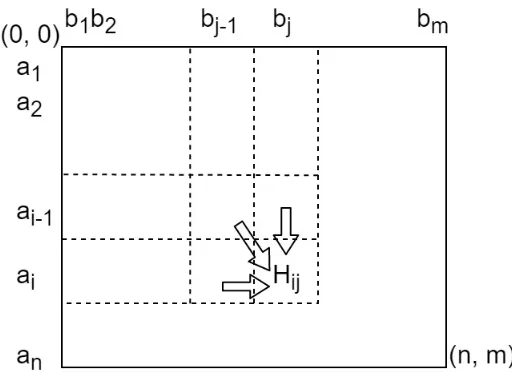
2.1 A matrixHis created to split sequence alignment problem into smaller problems. Suppose we have sequencesA = a1a2...an andB = b1b2...bm, where 0 < i  n

and 0 < j _ m. At any position (i, j) during dynamic programming, the

alignment path can come from (i 1, j), (i, j 1) and (i 1, j 1). All the candidates will be extended to containai and bj, and the similarity scores or

distances will be accumulated, the one with higher similarity degree will be kept for next dynamic programming steps. . . 6

2.2 Suppose the similarity scores for regions AB, BC andCD are 100, 120 and 110 respectively. If negative scores can be stored in H, at position C the similarity score will be 20, and 90 for positionD; therefore, the optimal local alignment would be regionAB, since it is the highest score. However, we know regionCDis a better solution with a higher score. Smith-Waterman solved this problem by setting all negative scores to 0 (positionCwill store value 0), then the similarity score forCDcan be obtained correctly. . . 8

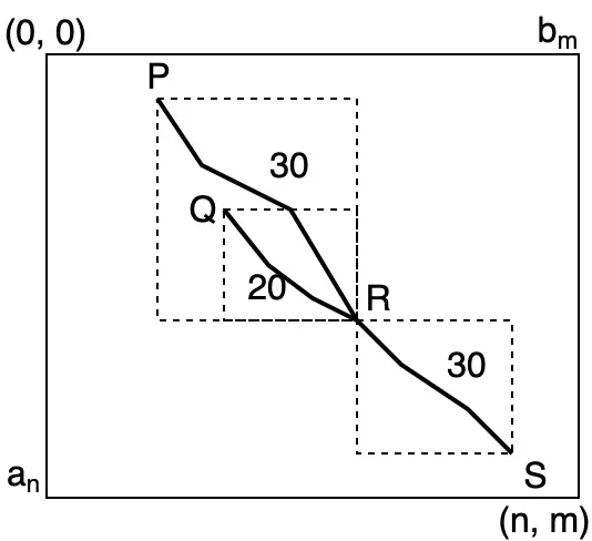
2.3 For any two sequences A = a1a2...an and B = b1b2...bm, suppose we know

there are two alignment PRand QR ending at Rwith similarity score 30 and 20 respectively, and the alignmentRS start fromRhas score 30, then alignment PS always provide higher additive score thanQS. In this example, the cumulative score forPS is 60, but 50 forQS. Therefore, Storing the highest score alignment at eachHi,j is enough for Smith-Waterman to find optimal alignment. . . 10

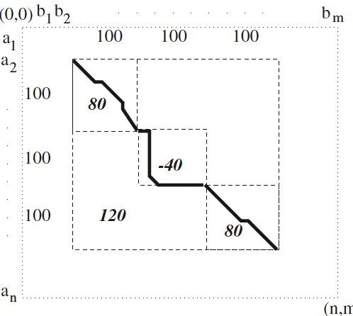
2.4 Mosaic e↵ect. The local alignment which is found by the Smith-Waterman algorithm has a score 120, and the scale is 300⇥300. The whole alignment is composed of three segments, two with score 80 and scale 100⇥100, the other one with score 40 and scale 100⇥100 as well. For some applications, only the consistently similar regions are required, such as the two regions with score 80, so that the internal segments with score 40 is useless, but Smith-Waterman will not decompose them into three pieces. . . 11

(8)

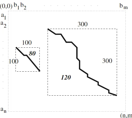
result. That means the low score alignment may have much higher similarity degree than the ”optimal” one; however, Smith-Waterman only targets to find the alignment with the highest similarity score, so another biologically meaningful region will be discarded. . . 12 2.6 Shadow e↵ect with overlapping. Smith-Waterman will take the alignment

path which can obtain a higher similarity score 120, rather than a much shorter path with score 80. . . 13 2.7 This is an example of phylogenetic tree built by complete mtDNA sequences

using frequency of k-mers [13]. . . 16 2.8 (a) is the original distance matrix obtained from sequences comparison; (b) is

the Qvalues calculated by equation 2.3 based on (a), for example, Q(a,b) =

(4 2)⇥6 (6+6+5) (6+7+6) = 24; (c) is the distance matrix after

joining, andd(u,c) andd(u,d) are obtained by equations 2.4, 2.5 and 2.6. . . . 17

3.1 (a) shows the weight function of each pair. (b) shows the result of post-normailzation. The path with minimum weight has been obtained firstly with value 6, and ˆW(P) is equal to 1.5 since L(P) is 4; however, it is not the path

with actual minimum normalized distance. The ideal path is shown in (c), with normalized distance 1.33 [14]. . . 20

3.2 The editing graphGX,Y for the stringsX = abaandY =bab. [2] . . . 23

3.3 a+cis the distance ofX andY, andbis the similarity. . . 32

3.4 Example of concave functions. L1,L2andkare constants, whereL>0 andk 1. 33

4.1 Any two alignments ending at the same position can have two di↵erent shapes based on their segment lengths. In 4.1a, neither of the alignment shapes fully contains the other one. Extending both alignments toC1 andC2could give the

opposite result, so either of them can be rejected at positionC. In 4.1b, the subsequences of alignmentQfully contain the segments ofP. If the similarity score ofQis lower, then no matter how the alignment extends,Qwill not give better solution so that it can be discarded at positionC. . . 44 4.2 The general shapes of alignments ending at position (i, j). Suppose there are

three candidatesO,PandQending at (i, j), then the segment lengths forPare xoandyo. Also, xp andypforP, xq,yq forQ. . . 49

5.1 Human mitochondrial DNA gene map [5]. . . 61 5.2 An example of fasta file, the first line is file description, and the rest lines are

the sequence of the particular protein which is inside the square bracket at the end of the description. . . 61 5.3 Rounded BLOSUM62 table, obtained from NCBI. . . 62 5.4 Two sequences of protein ATP6, one is from human and the other one is from

cat. . . 63

(9)

5.5 By applying multiple concave functions, the solutions have di↵erent similarity degrees. The solution generated by the Smith-Waterman algorithm is identical with the original sequences. . . 64 5.6 For alignment of sequenceXandY, we can getL1andL2length, but if changing

sequence Y to Z, new L1 will be obtained corresponding to the new optimal

alignment. . . 65 5.7 Phylogenetic tree of 20 mammals, the protein sequences were trimmed by the

new approach. and the distances were used by neighbor joining are normalized. Similarity metric isBLOSUM62. . . 67 5.8 This Phylogenetic tree used the trimmed protein sequences which were generated

by Smith-Waterman Algorithm, and the distances used by neighbor joining were not normalized. . . 68

(10)

List of Tables

3.1 The weight function which makes post-normalization fail triangular inequality. 21 5.1 amino acids table. . . 60

(11)

Chapter 1 Introduction

Let ⌃ denote a finite alphabet with space, and ⌃⇤ be the set of all finite-length string over

⌃. For any two elements xand y from⌃, let s(x,y) denotes the score of aligning x and y, if

they are identical or similar, a positive s(x,y) will be given for amatch, which could be two

identical nucleotides for DNA sequences alignment or both identical and very similar amino acids for protein sequence alignment; meanwhile, s(x,y) could be negative for penalizing a

mismatch (two irrelevant elements) or aligning one alphabet with space. Suppose we have stringsA=a1a2...amandB= b1b2...bn with lengthmandnrespectively. If spaces are inserted

into bothAand Bto get sequencesA0 ₌ _a0

1a02...a0Land B0 = b01b02...b0Lwith same lengthL, and

additive similarity score s(A0_,_B0₎ ₌ PL

i=1s(a0i,b0i) (such a similarity metric is called additive

similarity metric), then sequence alignment is to find A0 _and _B0_{, which generate maximum} s(A0_,_B0_{). For example, in}_Figure_1.1,_X_and_Y_{are two DNA sequences, where}_X ₌ _”_ACAGTC_”

andY = AGATCT. The naive alignment shows inFigure1.1a is to do nothing and align every

two letters at the same position from XandY, respectively. On the other hand, spaces can be inserted to gain more matches, likeFigure 1.1b. 1.1b aligned the sequence better, or we say alignment shown in 1.1b has higher similarity degree(percentage of matches) than 1.1a. In this thesis, if an element is aligned to space, the pair is called anindel.

Sequence alignment is widely used in bioinformatics and biostatistics, in order to find the homology or common ancestor through DNA or protein sequences from di↵erent species or individuals. There are two kinds of sequence alignment for di↵erent purposes: global

(12)

(a) Naive alignment (b) Better alignment solution

Figure 1.1: X = ”ACAGTC” and Y = AGATCT, there are many ways to align these two

sequences, the optimal solution is with most matches and as fewer mismatches as possible.

alignment and local alignment. A global alignment attempts to align each residue in the input sequences, and the result can show how close the input sequences are. On the other hand, a local alignment focuses on finding high similarity degree regions of sequences; it is usually used in aligning protein sequences to find homology.

There are two kinds of metric can be employed to measure how good alignments are: similarity metric and distance metric. Both of them quantify matches and mismatches of pairs, then sum up the scores for all aligned pairs to obtain the total distance or similarity score, so that di↵erent alignments can be compared. The similarity score for any single residue alignment can be positive or negative, but all scores are no less than 0 for distance metric.

In 1965, Soviet mathematician Vladimir Levenshtein proposed the first algorithm for sequence alignment all over the world, named Levenshtein Distance. It is a string metric and tries to minimize the single-character editing number to modify one string to the other [10].

(13)

3

during dynamic programming; so whenever a positive score appears, it is the start point of a local alignment. After all, the position, which contains the highest score, is the endpoint of the optimal local alignment [17].

Nowadays, Smith-Waterman is a popular algorithm for finding sequence local alignment, and are widely adopted in many applications; However, similarity score was the only criterion in this algorithm to select alignment pattern, regardless of the path’s length. The purpose of this algorithm is to find the highest score alignment which cannot be extended on both sides; therefore, if a poorly conserved segment is surrounding by well-aligned subsequences, the algorithm will consider them as one entire alignment, since the aggregate similarity score is the highest. For example, it has been discussed in [3] that when comparing long genome sequences, the output given by Smith-Waterman may not be ideal.

Notice that for any two sequences A = a1...an and B = b1...bm, if an alignment is found

with segments A0 ₌ _a

g...ai and B0 = bh...bj, then we denote the length (element numbers)

of A0 _as _x-length_{, and the length of} _B0 _{to be} _y-length_{. To solve the above problem, both} x lengthandy lengthshould also be considered to evaluate the alignment. For example, if

there are two local aligned patternsXandYfrom the same genomic sequences A=a1...anand B = b1...bm, the scores of X andY are 100 and 80 respectively, the x lengthandy length

of X are both 120, but alignmentY has both x length andy length 50. In this situation, patternY will be discarded by the Smith-Waterman algorithm, but it is obvious that elements are more consistently similar in patternY than in X. There might be small segments in pattern X, which are not biologically homologous. Due to these, sometimes, pattern Bneed also be

(14)

The similarity normalization strategy is to find sequence local alignment with higher similarity degree than the solution provided by the Smith-Waterman algorithm, but for two fixed input sequences, the higher the output similarity degree is, the shorter the alignment length will be. Therefore, for di↵erent applications, di↵erent normalization functions need to be applied for the same two sequences due to the di↵erent similarity degree requirements. Since most existing algorithms for finding sequence local alignment are based on dynamic programming which consumes a significant amount of time, when applying multiple normalization functions, dynamic programming will be executed multiple times, it leads to massive time consumption.

In order to obtain proper local alignments, we extended the idea of Smith-Waterman to design a dynamic programming algorithm to find optimal sequence local alignment. We used the normalized similarity metric family which is constructed by Minkowski type distance metric to find optimal solutions for di↵erent similarity degree requirements. Also, our algorithm only needs to run once, no matter how many normalization functions are applied since all useful data are kept during each dynamic programming run.

(15)

Chapter 2 Background

Sequence global alignment is a very basic idea to align two sequences and measure the similarity degree. The idea was extended to find sequence local alignment, and one of the most famous methods is the Smith-Waterman Algorithm. Later on, people noticed that only similarity score is not enough to find consistently similar local alignment; therefore, segment lengths has been considered for normalizing similarity score, aiming to find alignments that are consistently similar. At the same time, distance and similarity metrics have been well defined. Furthermore, since our experiment is to build a phylogenetic tree by the neighbor-joining method, a brief introduction of phylogenetic tree will be given at the end of this chapter.

2.1 Sequence Global Alignment

Sequence global alignment is to find the best arrangement, which can most efficiently align two sequences (achieve the highest similarity score or smallest distance). Specifically, every residue from the compared sequences must be aligned with space or a residue from the other sequence. Suppose we have sequences A = a1a2...an and B = b1b2...bm, where 0 < i  n

and 0< j _ m. In terms of finding optimal global alignment, dynamic programming split the

problem into subproblems. A matrix shown inFigure2.1 can be built to keep optimal global alignment scores for subsequences A0 ₌ _a

1a2...ai and B0 = b1b2...bj at each position (i, j).

Notice that at the very first row and column, all similarity scores are negative (or positive for

(16)

using distance metric) except value 0 at (0,0), because whenever a residue is aligned to space,

agap penalty with negative value should be given for using similarity metric. When we add spaces at the beginning of one sequence, the gap penalties will accumulate from position (0,0)

to (0,m) and (n,0). Then at each position (i, j) during dynamic programming, the alignment

candidates from (i 1, j), (i, j 1) and (i 1, j 1) will be extended by one more residue

alignment, and the highest similarity score will be stored for calculating the rest part of matrix H. Eventually, the one stored in position (n,m) in matrixHwill be the score of optimal global

alignment.

Figure 2.1: A matrixH is created to split sequence alignment problem into smaller problems. Suppose we have sequencesA = a1a2...anand B= b1b2...bm, where 0 < i nand 0< j  m.

At any position (i, j) during dynamic programming, the alignment path can come from (i 1, j),

(i, j 1) and (i 1, j 1). All the candidates will be extended to contain ai andbj, and the

similarity scores or distances will be accumulated, the one with higher similarity degree will be kept for next dynamic programming steps.

2.2 Sequence Local Alignment

(17)

2.3. Smith-WatermanAlgorithm 7

to satisfy the distinguishing requirements for applications. For instance, the Smith-Waterman algorithm always finds the segment pair with the highest similarity score, for those applications which require the optimal local alignment to be the segment pair with maximum score, the Smith-Waterman algorithm is e↵ectively. However, if the application needs the segment pairs which are strictly identical, the similarity score of optimal solution could be much smaller than the alignment found by the Smith-Waterman algorithm, which is more tolerant for mismatches (mismatches are accepted if they do not lower down similarity score below 0).

2.3 Smith-Waterman Algorithm

In the past half-century, along with more genes and proteins sequences of di↵erent species that have been decoded, people kept trying to develop new approaches to analyze the vast amount of sequence data. Before the Smith-Waterman algorithm was proposed, it was a tough task to find the homologous segments from long sequences, because along with the evolution, mutations and variations of DNA sequences always make too much noise along with the alignment. In 1981, based on global alignment approaches, the Smith-Waterman algorithm which is a dynamic programming algorithm was developed to find a pair of segments, from two given long sequences, such that there is no other pair of segments with greater similarity score (homology)” [17]. That means the optimal local alignment cannot be extended on both sides to achieve a higher similarity score. The Smith-Waterman algorithm also generates matrixH, but at each position (i, j) inH (we denote it asHi,j), the data stored is the global alignment score,

which is maximum among all possible subsequence pairag...aiandbh...bj, where 0 <giand

0<h_ j. In this thesis, when we talk about alignment starting from position (g,h) and ending

at (i, j) in H, it means the optimal global alignment for subsequence pairag...ai and bh...bj.

Notice that in the algorithm of finding global alignment, Hi,j can be negative, but the

(18)

or after the mismatches can achieve higher similarity score than the whole piece. Meanwhile, if g = i and h = j, then that means there is no similar segment pair exists between input

sequences, such as DNA sequencesA = ”GGG” andB = ”TTTT”, that means the alignment

which is found by the Smith-Waterman algorithm can be two empty segments with similarity score 0. Meanwhile, any alignments with negative scores will not be more optimal than score 0; therefore, negative scores will not be stored in Hdue to these two reasons. When negative scores are obtained during dynamic programming, the Smith-Waterman algorithm will record the scores as 0; then the similarity scores are correctly represented the similar regions without being e↵ected by mismatches before them. An example is given inFigure2.2.

Figure 2.2: Suppose the similarity scores for regionsAB, BC andCDare 100, 120 and 110 respectively. If negative scores can be stored in H, at positionC the similarity score will be 20, and 90 for position D; therefore, the optimal local alignment would be region AB, since it is the highest score. However, we know regionCDis a better solution with a higher score. Smith-Waterman solved this problem by setting all negative scores to 0 (positionC will store value 0), then the similarity score forCDcan be obtained correctly.

(19)

2.3. Smith-WatermanAlgorithm 9

candidate is from Hi 1,j 1, the additive for similarity score will be s(ai,bj). Hi,j will take the

maximal value among them and 0. The relationship is shown in Equation 2.1.

Hi,j =max

8 >>>>> >>>>> >>>>> >< >>>>> >>>>> >>>>> >:

Hi 1,j 1+s(ai,bj),

Hi 1,j+ ,

Hi,j 1+ ,

0

(2.1)

where is a gap penalty. The Smith-Waterman algorithm only need to store one alignment with the highest score at eachHi,j, because Smith-Waterman only measures the similarity score. As

we know the score is cumulative, so that if more than one candidate are stored at any position (i, j), then the alignments with lower scores will not generate higher score alignment in the end.

Moreover, an example can be found in Figure 2.3. The time complexity of Smith-Waterman is O(mn) because, at each position (i, j), the comparison part consumes fixed time.

The significance of the Smith-Waterman algorithm is undoubted; however, in the following three scenarios, Smith-Waterman may provide inefficient alignment solutions due to its properties [3].

Firstly, the optimal solution can include poorly aligned segments, and it is called mosaic e↵ect [3]. As long as the poorly aligned region cannot lower down the accumulative similarity score under 0 like shown inFigure 2.2, the whole piece will achieve the highest score. It is an optimal solution by the definition of Smith-Waterman, but it is not an ideal solution for all applications which may require more consistently similar alignment. The example is shown in Figure2.4 [3].

(20)

Figure 2.3: For any two sequences A = a1a2...an and B = b1b2...bm, suppose we know there

are two alignment PR and QR ending at Rwith similarity score 30 and 20 respectively, and the alignmentRS start fromRhas score 30, then alignmentPS always provide higher additive score thanQS. In this example, the cumulative score forPS is 60, but 50 for QS. Therefore, Storing the highest score alignment at eachHi,j is enough for Smith-Waterman to find optimal

alignment.

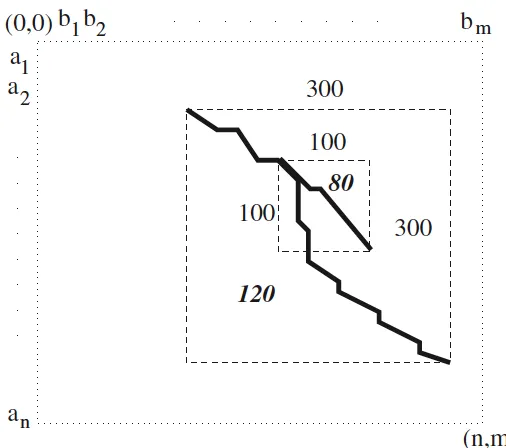
The third problem is similar to the previous one, the alignment could take another path to an endpoint with a little low score, but much shorter, but Smith-Waterman was designed to take the path which can generate the highest similarity score. SeeFigure 2.6 [3] for an example.

Briefly, Even though Smith-Waterman is an efficient algorithm to find local alignment, it is not flexible for all applications to find corresponding ideal solutions, since the only criterion Smith-Waterman takes to measure alignments is similarity score.

2.4 Similarity Metric

Similarity metric is widely used in many areas, such as protein sequences comparison. The definition is given in [7] in 2007, and is stated below:

(21)

2.4. SimilarityMetric 11

Figure 2.4: Mosaic e↵ect. The local alignment which is found by the Smith-Waterman algorithm has a score 120, and the scale is 300⇥300. The whole alignment is composed of three segments, two with score 80 and scale 100⇥100, the other one with score 40 and scale 100⇥100 as well. For some applications, only the consistently similar regions are required, such as the two regions with score 80, so that the internal segments with score 40 is useless, but Smith-Waterman will not decompose them into three pieces.

a similarity metric if,8a,b,c₂X, it satisfies the following properties:

1. s(a,b)= s(b,a)

2. s(a,a) 0

3. s(a,a) s(a,b)

4. s(a,b)+s(b,c)_ s(b,b)+ s(a,c)

5. s(a,a)= s(b,b)= s(a,b) if and only ifa= b

Furthermore, we say a similarity metric s(a,b) is a normalized similarity if

(22)

Figure 2.5: Shadow e↵ect without overlapping. There is another alignment with score 80, which is lower than 120, but its scale is much smaller than the algorithm result. That means the low score alignment may have much higher similarity degree than the ”optimal” one; however, Smith-Waterman only targets to find the alignment with the highest similarity score, so another biologically meaningful region will be discarded.

2.5 Distance Metric

Let⌃be a set of finite characters including space, and (a,b) be a string pair of any finite length

from ⌃. Then an edit operation could be to substitute a with b, insertion or deletion. The penalty of each edit operation can be assigned by distance metric function , which has to satisfy the following conditions:

1. (a,b)= (b,a),

2. (a,b) 0,

3. (a,c)_ (a,b)+ (b,c) (triangle inequality),

4. (a,b)=0, if and only ifa=b.

(23)

2.6. Similarity andDistanceMetricNormalization 13

Figure 2.6: Shadow e↵ect with overlapping. Smith-Waterman will take the alignment path which can obtain a higher similarity score 120, rather than a much shorter path with score 80.

From distance metric condition 4, it is obvious that if sequences XandY are identical with infinite elements, the total distance for these two sequences will be 0 forever, by adding the distance of each element pair. In this case, if one base in X has been modified to another alphabet, then the distance of X and Y equal to the distance of the particular base pair. For example, if Xi was changed from ”a” to ”b”, the distance of two infinite length string would

be (Xi,Yj), which is (b,a). Meanwhile, suppose we have another two strings MandN with

length 1 for both, where M = ”b” and N = ”a”. Then the distance for M and N will be the

same as the distance of X andY; however, over 99% base pair of X and Y are the same, and M has no relationship with N at all. To avoid this problem, the alignment length needs to

be considered in order to normalize distance. The detail algorithms will be introduced in the following chapter.

2.6 Similarity and Distance Metric Normalization

(24)

Definition Similarity metrics(a,b) is normalized similarity metric if_|s(a,b)_|_1.

The only measurement needed for global alignment is similarity score or distance because all the possible alignments must include every residue from both sequences, which means all possible alignments have the same length. Therefore, for any two fixed sequences, the optimal global alignment must be the one with the highest similarity score or smallest distance.

For finding local alignment, at each dynamic programming step, we cannot reject lower score alignment. Because at the specific point, candidates can have di↵erent starting points, so the alignment with a lower score may have much shorter lengths than another candidate with a higher similarity score. Also, since the local alignment length is flexible, then there could be a great number of similar segments combinations exist. Notice that for each found individual local alignment, it is the optimal global alignment among all candidates from the corresponding segment pair with fixed starting and ending points; however, its similarity degree may be less than another local aligned segment pair, so it has to be rejected. Briefly, both segment lengths and similarity score need to be considered, and it is much more complex than global alignment. Therefore, how to make rejection decision and find the most similarity segment pair become the most controversial issue for the local alignment problem. The very basic idea is to reject those alignments with lower similarity scores and including more residues (longer length) at the same time, but except those obvious inefficient candidates, there are still many lefts. In the past decades, people proposed many algorithms that attempted to e↵ectively normalize similarity scores by alignment lengths for making rejection decisions, and chapter 3 will give details of di↵erent normalization approaches.

(25)

2.7. Neighbor-joining andPhylogeneticTree 15

2.7 Neighbor-joining and Phylogenetic Tree

According to the studies of di↵erent organisms, it is speculated that all creatures on the earth had one common ancestor, and the evolutionary relationships have been studied for many years. For di↵erent species, the relationships can be represented by a phylogenetic tree, which is an acyclic graph. Each leaf node of the tree stands for one particular organism, and the edges’ lengths (or the weights) are the distances among species. Figure 2.7 is an example of phylogenetic tree, and it is observed that gibbon and orangutan, grey seal and harbor seal, opossum platypus are clustering as branches firstly, this situation can be interpreted as those three pairs of species are closely related respectively. A phylogenetic tree can be rooted or unrooted, where unrooted tree does not make any prediction for ancestor, it only shows the evolutionary distances. Since we constructed unrooted tree for experiments, all phylogenetic trees which are mentioned will be unrooted in the rest of this thesis.

Neighbor-joining is one of the most popular methods for constructing phylogenetic tree, and it was proposed in 1987 [16]. The main idea of this method is to iteratively join two particular taxa and gain a new graph that has less total distance than any other joining combination and reduce the taxa set by one. For example, in order to build a phylogenetic tree which includes n species, where d(i, j) denotes the distance between any two taxa, the algorithm

always try to find minimumQin each iteration [11]:

Q(i, j)=(r 2)d(i, j) r

X

k=1 d(i,k)

r

X

k=1

d(j,k) (2.3)

whereris the current taxa number. After finding optimal joining combination, an internal node uwill be created to join these two taxa (suppose they are f andg). Then:

d(f,u) = 1

2d(f,g)+ 1 2(r 2)[

r

X

k=1

d(f,k) r

X

k=1

d(g,k)] (2.4)

(26)

Figure 2.7: This is an example of phylogenetic tree built by complete mtDNA sequences using frequency of k-mers [13].

After joining, the distance fromuto any other taxakneed be calculated for next iteration, anduwill replace taxa f andgin the distance matrix.

d(u,k)= 1

2[d(f,k) d(f,u)]+ 1

2[d(g,k) d(g,u)] (2.6)

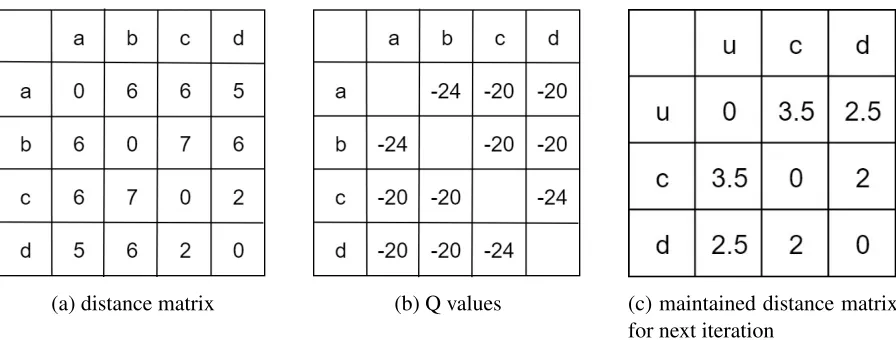
For example, if we have four speciesa,b,candd, with distances between any pair of them,

then we have the distance matrix inFigure2.8a. Firstly,Q(i, j) will be calculated to generate

Figure2.8b; also sinceQ(a,b) and Q(c,d) have the same value, we can either joina,borc,d.

(27)

2.8. Red-blackTree 17

(a) distance matrix (b) Q values (c) maintained distance matrix

for next iteration

Figure 2.8: (a) is the original distance matrix obtained from sequences comparison; (b) is the Q values calculated by equation 2.3 based on (a), for example, Q(a,b) = (4 2)⇥6 (6+

6+5) (6+7+6) = 24; (c) is the distance matrix after joining, andd(u,c) andd(u,d) are

obtained by equations 2.4, 2.5 and 2.6.

orb. After joining, the new distance matrix inFigure 2.8c needs to be generated for the next joining iteration.

2.8 Red-black Tree

A red-black tree is a binary search tree. Another attribute is added in each tree node to indicate the node color, in order to make the tree self-balancing. A red-black tree must have the following properties:

1. The color of root node must be black.

2. Each node must have color red or black.

3. Every leaf node must be black.

4. The children of a red node must be black.

(28)

When a new node is inserted into the tree, a series of rotations must be taken to maintain the tree, in order to satisfy the above properties. Therefore, we get the following lemma [18], and the proof can be found on the page: [18, p. 309]:

(29)

Chapter 3 Literature Review

3.1 Normalized Editing Distance

In the 1990s, many algorithms have been developed to fix the mosaic e↵ect, such as theX alignmentsmethod, where Xis a predetermined and fixed positive integer, the alignment will

be considered, if the score does not drop more than X [21]. Later on, Zhang et al. tried to decompose the local alignment into sub-alignments [22]; however, if the highly aligned parts are split into di↵erent subsequences, they could be missed, since the segments may not win out in the corresponding subsequences. At the same time, normalizing distance or similarity score has been considered.

In 1993, one of the earliest normalization algorithms was published by Andres Marzal and Enrique Vidal [14]. In the paper, they provided a well-designed algorithm to find the normalized editing distance inO(m_⇥n2_{) time and}_O₍_n2_{) memory space, where}_m_and_n_{are the}

input sequence lengths, andm n. Furthermore, they explained that normalized distance could not be calculated by firstly getting the minimum weight path, then use the length to normalize it.

Suppose the editing path P = (i0, j0)...(im, jm) with length L(P) = m, then the general

formula to calculate normalized distance ˆW(P) is:

ˆ

W(P)= W(P)

L(P), (3.1)

(30)

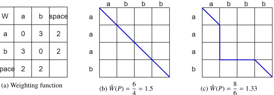
(a) Weighting function _{(b) ˆ}_W₍_P₎₌ 6

4 =1.5 (c) ˆW(P)=

8

6 =1.33

Figure 3.1: (a) shows the weight function of each pair. (b) shows the result of post-normailzation. The path with minimum weight has been obtained firstly with value 6, and

ˆ

W(P) is equal to 1.5 sinceL(P) is 4; however, it is not the path with actual minimum normalized

distance. The ideal path is shown in (c), with normalized distance 1.33 [14].

whereW(P) is the weight of pathP. Therefore, the normalized editing distance between string X andY is:

d(X,Y)=min{Wˆ(P)|P is an editing path between X and Y} (3.2)

The minimization step is to compare the normalized weights of paths with di↵erent lengths and find the minimum one, and it has been proved that the minimization step cannot be carried out before normalization. The following example can show the reason.

Given string X = abbb, Y = aaab, and the weight function is shown inFigure 3.1a. If

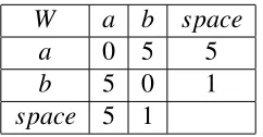
the minimization step is carried out after the dynamic programming, indeed the resulting path is the one with minimum weight, but since the path lengths are not the same, the normalized weight may not be the minimum as well. The path shown in Figure 3.1c is the path with minimum normalized distance. Also, theoretically, the post-normalization method does not satisfy condition 3 (triangular inequality) of distance metric, which was given in chapter 2. For example, if the weight function in Table 3.1 is used, and X = a, Y = ab and Z = b. The

ˆ

W(P) forXandYis 1 2, and

5

2 forY andZ; however, The ˆW(P) forXandZis 5

1. Now we have 1

2+ 5 2 ↵

5

(31)

3.1. NormalizedEditingDistance 21

be 6

2, then the inequality hold again.

W a b space

a 0 5 5

b 5 0 1

space 5 1

Table 3.1: The weight function which makes post-normalization fail triangular inequality.

In order to get d(X,Y), the naive way would be to list all the paths between X and Y,

then calculate the normalized weight for each of them; however, it is too expensive to do so. SupposeX = X1X2...Xn, Y = Y1Y2...Ym, andn m, then the length of editing path betweenX

andY should be in the range [n,m+n]. Hence, during dynamic programming, at any position

(Xi,Yj), wherei  jthere will be i+ 1 paths with di↵erent lengths are calculated and saved.

For each length, the calculation is shown in the followingTheorem [14]:

Theorem 3.1.1 8i, j,1 _ i _ _|X_|,1 _ j _ _|Y_|,₈k,max(i, j) _ k _ i+ j, let (a ! b) be the

editing operation weight function to transfer a to b.

D(i, j,k)= min{D(i 1, j,k 1)+ (Xi ! ),D(i, j 1,k 1)+ ( ! Yj),D(i 1, j 1,k 1)+ (Xi ! Yj)}

D(i, j,k)= 1,₈k_max(i, j),₈k i+ j

FromTheorem 3.1.1, it is known that the time complexity of calculatingD(i, j,k) isO(1).

So that the time complexity of getting all lengths path at position (Xi,Yj) isO(N), which isO(m)

(32)

Algorithm 1Normalized editing distance

Input: X =X1X2...Xn,Y = Y1Y2...Ym, weight function (a!b);

Output:d(X,Y)

1: int i, j,k

2: D[_|X_|,_|Y_|,_|X_|+|Y|+1] is a 3D array

3: D[0,0,0]=0

4: D[0,0,1]=1

5: for j=1! |Y|do

6: D[0, j, j 1]=1

7: D[0, j, j]=D[0, j 1, j 1]+ ( !Yj)

8: D[0, j, j+1]=1

9: end for

10: fori= 1!|X|do

11: D[i,0,i 1]=1

12: D[i,0,i]= D[i 1,0,i 1]+ (Xi ! )

13: D[i,0,i+1]=1

14: for j=1!|Y|do

15: D[i, j,max(i, j) 1]=1

16: fork=max(i, j) toi+ jdo

17: D[i, j,k] =min(D[i 1, j,k 1]+ (XI ! ),D[i, j 1,k 1]+ (yj ! ),D[i

1, j 1,k 1]+ (Xi !Yj))

18: end for

19: D[i, j,i+ j+1]=1

(33)

3.2. An improvement ofNormalizedEditingDistance 23

3.2 An improvement of Normalized Editing Distance

As mentioned, the time complexity of the previous algorithm is O(mn2_{), if} _m _and _n _{are the}

lengths of sequenceXandY, respectively, andm n. In 1999, Abdullah N. Arslan and Omer Egecioglu [2] proposed an improved algorithm that requires O(mnlogn) time, if the cost of the same type of editing operation is uniform. Instead of calculating normalized weight along with the dynamic programming, this algorithm only solves ordinary editing distance problem at most logntimes.

A graph could be used to describe the ordinary problem, just like 3.2. An editing path of string X andY is from vertices (0,0) to (m,n), and can go to three directions corresponding

to three di↵erent operations which are deletion (if goings horizontally), insertion (if going vertically) and substitution (if going diagonally). Also, the cost function is =( I, D, M, N),

which Iis the cost for insertion, Dfor deletion, M for matching substitution and N for

non-matching substitution. The assumption is that all of them are constant.

(34)

LetW (p) denote the weight of editing path p, andh(p) be the horizontal move number of path p, v(p) be the vertical move number, dN(p) is the non-matching diagonal move number

anddM(p) be the matching diagonal move number. Then:

W (p)= Dh(p)+ Iv(p)+ MdM(p)+ NdN(p), (3.3)

The length of path pis:

L(p)= h(p)+v(p)+dM(p)+dN(p), (3.4)

We also have:

m = h(p)+dM(p)+dN(p) (3.5)

n = v(p)+dM(p)+dN(p) (3.6)

Therefore,W (p) and L(p) can be transformed to:

W (p) = D+n I+( M I D)dM(p)+( N I D)dN(p) (3.7)

L(p) = m+n dM(p) dN(p) (3.8)

Recall the normalized editing distance is:

N E Dx,y, = min p2P

W (p)

L(p) , (3.9)

(35)

3.2. An improvement ofNormalizedEditingDistance 25

N E Dx,y, =min p2P

D+n I+( M I D)dM(p)+( N I D)dN(p)

m+n dM(p) dN(p) . (3.10)

From the aboveEquation3.10, we can see finding NED becomes to optimize the ratio of two linear functions. In order to solve this problem, Dinkelbach’s algorithm [9] are used. The basic idea of this algorithm is fractional programming. The optimal solution of equation 3.10 can be achieved by solving Equation 3.11, where 2 R. ⇤ _{will be the optimal solution of}

Equation3.10, if and only if the optimal vaule of f( ⇤_{) is zero.}

f( ) =min[W (p) L(p)]. (3.11)

Noticed that, if we substituteW (p) andL(p) withEquation3.7 and 3.8, then 3.11 can be simplified to a new editing path weight function with new weights, and the variables aredM(p)

and dN(p). Instead of calculating NED through the dynamic programming, we just need to

try di↵erent by finite times to find the optimal value; therefore, the time consuming of this algorithm should beO(kmn), wherekis the number of trials. As we know,dM(p)+dN(p) cannot

be greater than the length of the shorter sequence, which isnhere; therefore, there should be n_⇥ncombinations ofdM(p) anddN(p), which corresponding ton2 candidates of . To make

it simple, that n2 _{values will be calculated in advance. Then the median candidate (let’s say}

ˆ) value can be picked for first trial, after finding the minimum weight editing path, if f(ˆ)) is greater than 0, that means the ⇤ _{should be greater than ˆ), then all the candidates smaller}

than ˆ) can be ignored, vice versa, until it reaches zero. In each iteration, the range will be divided into half, then the worst case would be logn2_{iterations. In other words, k is}_O_(log_n_).

Combining the time of building possible set, the time complexity of the whole algorithm is O(n2₊_mn_log_n_{), which is}_O₍_mn_log_n_{). The main steps of this algorithm is shown in}_Algorithm

(36)

Algorithm 2NED algorithm for uniform weights

Input: X =X1X2...Xn,Y = Y1Y2...Ym, weight function

Output: ⇤

1: if m=n= 0then

2: return 1

3: end if

4: if m=0then

5: reuturn I

6: end if

7: if n=0then

8: return D

9: end if

10: Generate the setQof 11: whiletruedo

12: Find the median medofQ

13: SolveE DX,Y, ( med)

14: ifthe minimum path weight is 0then

15: return med

16: else

17: ifthe minimum path weight is smaller than 0then 18: remove the values equal and larger than med

19: else

20: remove the values equal and smaller than med

21: end if

(37)

3.3. NormalizedLocalSimilarityScore 27

3.3 Normalized Local Similarity Score

In order to find similar segments between DNA sequences of di↵erent species, local alignment algorithm must be used. In 2000, [3] extended the idea of uniform weight normalized editing distance algorithm [2], which was just discussed above, to normalize the similarity score. Suppose we have string X and Y, I and J are the substrings for X and Y respectively. The basic idea is to find the maximum value of s(I,J)/(_|I_|+|J|), where |I|+|J| T andT is the

threshold for alignment length. However, those alignments with high similarity degree but very short length will be obtained by this formula, the result is biologically meaningless. To fix this problem, they add a constant numberLto the denominator. Thenfractional programmingwill be used to find the optimal alignment.

As mentioned in the last section, an alignment can be considered as a graph, and the similarity score can be calculated by three values: number of matches, mismatches and indels (insert or deletion). Suppose the score for a match is 1, for a mismatch and µ for indel.

Therefore, vector (x,y,z) can be used to represent a local alignment withxmatches,ymismatches

andzindels. Then the similarity score is:

S CORE(x,y,z)= x y µz (3.12)

The best alignment between substringsai...akandbj...bkwould be the vector with maximum

score among all the alignment vectors between these two strings. Furthermore, the optimal local alignment of strings a and b is to seek for two substrings ai...ak and bj...bl, with the

highest similarity score, letLA⇤_{be the score of optimal local alignment, then:}

LA⇤₍_a_,_b₎₌ _max_{_{S CORE}₍_x_,_y_,_z₎_|₍_x_,_y_,_z₎_{is any alignment vector o f a}_i..._a

kand bj...bl}

(3.13)

(38)

2x+2y+z+L, whereLis the constant to control the optimal alignment length:

LENGT H(x,y,z)=2x+2y+z+L (3.14)

Therefore, the optimal normalized similarity score should be:

NLA⇤₍_a_,_b₎ ₌ _max_{ S CORE(x,y,z)

LENGT H(x,y,z)} (3.15)

= maximize x y µz

2x+2y+z+L (3.16)

Recall theparametric method,NLA_⇤(a,b) can be transferred to another ordinary similarity

problem:

LA( )(a,b)=maximize x y µz (2x+2y+z+L) (3.17)

Then the Smith-Waterman and Dinkelbach’s algorithm will do the rest work until find the optimal local alignment, just like the algorithm introduced in section 3.2. Later on, the author proved that the time complexity could be better if using Megiddo’s algorithm [2].

3.4 Similarity Metric and Normalized Similarity Metric

Recall the definition of similarity metric was given in [7] is:

Definition Given a setX, a real valued function s(x,y) on the Cartesian productX_⇥XofXis

a similarity metric if,8x,y,z₂X, it satisfies the following properties:

1. s(x,y)= s(y,x)

2. s(x,x) 0

(39)

3.4. SimilarityMetric andNormalizedSimilarityMetric 29

4. s(x,y)+s(y,z)_ s(y,y)+ s(x,z)

5. s(x,x)= s(y,y)= s(x,y) if and only ifx= y

Although similarity measure is used in many fields such as protein sequence comparison, there was no formal concept had been proposed until 2007 [7].

The first three conditions are intuitive, and condition four is similar to triangle inequality of distance metric. It states that the similarity between two elements through the third one is less than the actual similarity of these two elements plus the similarity of the third one comparing to itself. In addition, in order to understand condition 5, suppose we have s(x,y) that satisfies

the first 4 conditions of similarity metric, ands(x,x)= s(y,y)= s(x,y). For anyz, by condition

4, we have s(x,y)+s(y,z)_ s(x,z)+s(y,y). Sinces(x,y)= s(y,y), we can get s(y,z)_ s(x,z).

On the other hand, we also can have s(y,x)+s(x,z)_ s(y,z)+s(x,x), which can be simplified

tos(x,z)_ s(y,z). Therefore, we have s(x,z)= s(y,z), which meansxcan be treated asy.

The definition of normalized similarity metric is:

Definition A similarity metrics(x,y) is anormalized similarity metricif_|s(x,y)_|_ 1.

In [8], the authors also pointed out the method, which had been introduced in the previous section (_|_as_|₊(a,b_|_b_|₊)_L, where Lis a constant and L > 0 ), is not a similarity metric. It can be easily proved by a counter example. Suppose we have sequences X = ”abc”, Y = ”abcde” andZ =

”cde”, for any character pairiand j, we have scoring function s(i,i)= s(j, j)= 2, s(i, j)= 1

and 0 for any indels. We can sees(i, j) is a similarity metric,s(X,Y)= s(Y,Z)=6, s(Y,Y)=12

and s(X,Z) = 2. We also have|X|= |Z| = 3,|Y|= 5, and supposeL= 1. If we used _|_as_|+|(a,b_b_|+)_L to

normalize the scores, then we have _|_Xs_|₊(X,Y_|_Y_|₊)_L + _|_Ys_|₊(Y,Z_|_Z_|₊)_L = 6₉ + 6₉, and _|_Xs_|(₊X,Z_|_Z_|₊)_L + _|_Ys_|₊(Y_|_Y,Y_|₊)_L = 2₇ + 10₁₁.

It is clearly that _|_Xs_|(₊X,Y_|_Y_|₊)_L+ _|_Ys_|₊(Y_|_Z,Z_|₊)_L is larger than _|_Xs_|₊(X,Z_|_Z_|₊)_L + _|_Y_|s₊(Y,Y_|_Y_|₊)_L, so condition 4 does not hold

under this situation.

(40)

detail will be given in the following, with the definition of concave function. The proofs can be found in [20].

Definition A function f is concave over an interval [a,b] if for every x1,x2 2 [a,b] and 0 

 1,

f(x1)+(1 )f(x2) f( x1+(1 )x2) (3.18)

Lemma 3.4.1 if a function f is concave over interval ( 1,₁), then for any a, b 0 and c 0,

f(a)+ f(a+b+c) f(a+b)+ f(a+c). (3.19)

Lemma 3.4.2 Let f be a non-negative concave function on domain [0,₁), and 0 _ x _ y, b 0, then x

f(x+b) 

y f(y+b).

The paper [20] also defined Minkowski type similarity and distance metric for p 1.

Theorem 3.4.3 If s(x,y)is similarity metric, and p 1, then:

d(x,y)= pp(s(x,x) s(x,y))p+(s(y,y) s(x,y))p (3.20)

is a distance metric.

Lemma 3.4.4 If s(x,y)and d(x,y)are similarity and distance metric respectively, also satisfying normalization condition, and f(x)is a monotone increasing concave function on[0,₁), also

f(x)> 0. Then:

s(x,y)+ s(y,z) s(y,y)

f(d(x,y)+ s(s,y)+d(y,z)+s(y,z) s(y,y)) 

s(x,z)

f(d(x,z)+s(x,z)) (3.21)

Theorem 3.4.5 If s(x,y)and d(x,y)are similarity and distance metric respectively, also satisfying normalization condition, and f(x)is a monotone increasing concave function on[0,₁), also

(41)

s(x,y)= s(x,y)

f(d(x,y)+ s(x,y)) (3.22)

is a similarity metric.

In order to find sequence local alignment, a proper similarity metric is required. Smith-Waterman applied additive similarity metric, so it may not provide ideal solution in some scenarios. The metric shown inTheorem3.4.5 considers segment length when finding optimal solution, and it invokes concave function to control the similarity degree of solution; therefore, we consider the following similarity metric which satisfiesTheorem3.4.3 and 3.4.5 is proper for finding normalized sequence local alignment.

s(x,y)= s(x,y)

f(pp₍_s₍_x_,_x₎ _s₍_x_,_y₎₎_p

+(s(y,y) s(x,y))p₊_s₍_x_,_y₎₎, (3.23)

Where f(x) is a monotone increasing concave function on [0,₁), also f(x)>0.

Being di↵erent from other normalization functions,Equation3.23 quantifies both similar and dissimilar regions, rather than directly normalize the similarity score by the summation of two segment lengths. It can be easily understood by using set theory. We treat s(x,y) as the

common part of sequences xandy, it is shape bin Figure 3.3. Also, we can see shapeaand c are the non-common parts for sequences x andy respectively, so s(x,x) s(x,y) represent

shapeaands(y,y) s(x,y) for shapec, thend(x,y) can be interpreted asa+c. Therefore, we

usea+b+cto represent the union of sequencesxandy, which isd(x,y)+s(x,y). In addition,

di↵erent value ofkcan be chosen to calculated(x,y) for specific applications.

(42)

Figure 3.3:a+cis the distance ofXandY, andbis the similarity.

Figure 3.4 shows an example of concave functions, where f(x) = x + L1 is a special case

of a concave function. When alignment is short, L1 will be relatively large, so it e↵ectively

avoids obtaining very short alignments. However, notice that this function does not regulate variable x, so when the alignment gets longer, normalization strength still increases too fast to encourage longer alignment. On the other hand, g(x) = x1/k + L2 works better, because

its normalization strength is relative with the alignment length. Longer the alignment length is, slower the strength increases. Furthermore, if a concave function converges too fast, the denominator of normalization function will be like a constant; therefore, the solution will be close to, or even the same as the solution of Smith-Waterman Algorithm.

Let X andY be two sequences, then there are a great number of arrangement patterns for them with di↵erent similarity scores. Let A(X,Y) denotes the additive similarity score for an

alignment, then among allA(X,Y), the highest one is the score of optimal global alignment for X andY, and denoted ass(X,Y). Specifically,

s(X,Y)=max

all A A(X,Y). (3.24)

(43)

Figure 3.4: Example of concave functions. L1,L2andkare constants, whereL>0 andk 1.

A(X,Y)= A(X,X)

f(pp₍_s₍_X

,X) A(X,Y))p₊₍_s₍_Y_,_Y₎ _A₍_X_,_Y₎₎p₊_A₍_X_,_Y₎₎, (3.25)

where s(X,X) and s(Y,Y) are the optimal global alignment scores for aligning X andY to

themselves. Then we have:

s(X,Y)=max

allA A(X,Y). (3.26)

Therefore, the normalized similarity metric shown in 3.23 has following lemma:

Lemma 3.4.6 For any finite sequences X and Y, let s(X,Y) denotes the additive similarity score of optimal global alignment, and s(X,Y) denotes the normalized similarity score of

optimal alignment by applying normalized similarity metric showing in Equation3.23, then

the alignment generating s(X,Y)will always generate s(X,Y)as well.

(44)

s2(X,Y) respectively, wheres1(X,Y) s2(X,Y), then byLemma3.4.2, we have:

s1(X,Y)

f(b+s1(X,Y)) 

s2(X,Y)

f(b+s2(X,Y)), (3.27)

whereb 0. If 0<c_ b, then

s2(X,Y)

f(b+ s2(X,Y)) 

s2(X,Y)

f(c+ s2(X,Y)), (3.28)

since concave function f(x) is monotone increasing. So

s1(X,Y)

f(b+ s1(X,Y)) 

s2(X,Y)

f(c+ s2(X,Y)). (3.29)

Also since s1(X,X) and s2(Y,Y) are fixed, then:

p

(s1(X,X) s1(X,Y))p+(s1(Y,Y) s1(x,y))p  pp(s2(X,X) s(X,Y))p+(s(Y,Y) s(X,Y))p

(3.30)

Letb= pp(s1(X,X) s1(X,Y))p+(s1(Y,Y) s1(x,y))p,c= pp(s2(X,X) s(X,Y))p+(s(Y,Y) s(X,Y))p,

then fromEquation3.29 we have

s1(X,Y) s2(X,Y). (3.31)

Therefore, higher s(x,y) generate higher s(x,y).

In Lemma3.4.6, s(x,y) does not have to be additive similarity metric, but the algorithm

(45)

3.5. BLOSUM 35

3.5 BLOSUM

The protein sequence alignments are usually involved in order to study gene and protein function. No matter for global, local, or multiple sequence alignments, a scoring scheme must be invoked to measure the similarity degree. Before 1992, there are several scoring schemes have been proposed, and the most popular one is the mutation data matrices which were proposed by Dayho↵in 1968 [6]. In his model, the amino acid substitution rates are generated from protein sequences, which are aligned, and the similarity degree is above 85%. However, most tasks need to identify those distantly related segments by inferred from Dayho↵’s model which is derived from high similarity protein sequences. Therefore, BLOSUM was proposed to use di↵erent protein sequence alignments groups which have particular lower similarity degree within specified sequence blocks.

Until now, BLOSUM metric series is still one of the most common methods to measure the similarity of any amino acid pairs. The matrices are proposed by Steven Heniko↵ and Jorja G. Heniko↵in 1992 [12], and the content of BLOSUM matrices are the frequencies of corresponding amino acids are substituted by other amino acids, just like Dayho↵’s model.

Firstly, from a group of related proteins, a set of blocks will be found, and a system called PROTOMAT finishes this process. Each block is the most common region for the particular protein family. For example, if we have 5 protein sequences from the same family, and the block length is 3 amino acids, then the block size is 5⇥3. For each column, all the matches and mismatches for the corresponding amino acid pair will be counted. For example, if there are 4 A, and only oneBin the first column, thenAAappears 3+2+1= 6 times, 4 forABorBA, and

0 times forBB. The calculation for each column is summed up for a observed frequency table.

After counting, the probability of each amino acid pair will be calculated based on the table. For the same example, the 5⇥3 block can generate 3⇥5⇥(5 1)/2 = 30 pairs, and since

AA appears 6 times, then the observed probability of (A,A) is Pr(A,A) = 6/30 = 0.2, and

(46)

Pr(i, j)= _P₂₀ fi j

i=2

Pi

j=1 fi j

. (3.32)

Then, the expected probability thatiappears in any pair is:

Pr(i)= Pr(i,i)+X

j,i

Pr(i, j)/2. (3.33)

In the example, the expected probability ofAappears in a pair is 0.2+0.13/2=0.265, and

0.13/2= 0.065 forB. And then, the expected probability for any pair (i, j) is:

ei j = Pr(i)⇥Pr(i), i f i= j (3.34)

= Pr(i)⇥Pr(j)+Pr(j)⇥Pr(i), i f i, j. (3.35)

Eventually, the odds ratio can be got by:

si j =log2(Pr(i, j)/eij). (3.36)

If si j > 0, it means the pair appears more than expected, it will be multiplied by scaling

factor 2. Generally, the result will be rounded to the nearest integer, and it is how BLOSUM matrices are generated.

Furthermore, in order to reduce the frequency contribution from those protein sequences which are too closely related, such sequences will be clustered within blocks and contributed as one single sequence. There are di↵erent standards for clustering, such as BLOSUM62, it means that if sequences are identical more than 62% of their aligned positions, they will be clustered together. Without rounding, any BLOSUM-N matrix with N 55 is a similarity metric [20].

(47)

3.5. BLOSUM 37

s(x,y)= s(x,y)

f(pp₍_s₍_x

,x) s(x,y))p+(s(y,y) s(x,y))p+s(x,y)), (3.37)

is a similarity metric. Therefore, we used this method to normalize the similarity score, where s(x,y) is based on BLOSUM62. The reason we used the concave function is its slope

(48)

Chapter 4 A New Algorithm for Normalized

Sequence Local Alignment

Sequence local alignment is to find similar segments from input sequences, but ”similar” can be defined in di↵erent ways. For example, Smith-Waterman defines the optimal local alignment to be the one with the highest similarity score. Even though it is widely used in bioinformatics studies, it is not suitable for those applications which require consistently similar local alignment. In order to obtain segments with high similarity degree, normalization functions need to be invoked to take both similarity score and alignment length into account. Therefore, multiple normalization functions need to be applied on the same sequences for di↵erent similarity degree requirements, and it will consume a significant amount of time.

To solve these issues, we invoked the normalized similarity metric family [20] which are constructed by Minkowski type distance metric to satisfy di↵erent requirements for similarity degree. Then, a dynamic programming algorithm has been designed to find sequence local alignment. As introduced in chapter 2, algorithms which target finding sequence alignment will generate a matrix H. Our algorithm also produces matrix H, but the data stored in each Hi,j includes all alignment candidates which pass through (i, j) and have the possibility to

generate optimal solution. Therefore, no matter how many normalization functions from our similarity metric family are applied, the corresponding optimal solution can be obtained by iterating eachHi,j and applying normalization functions to process all alignment candidates.

We define the optimal local alignment to be the segment pair with the highest normalized

(49)

4.1. A SimpleAlgorithm for findingNormalizedSequenceLocalAlignment 39

similarity score. Specifically, for any two sequencesA = a1a2...an andB = b1b2...bm, we look

for subsequence pairA0 ₌_a_g..._a_i _and_B0 ₌_b_h.._b_j_{, where 0}_< _g_ _i__n_{and 0}_< _h_ _j __m_{, that}

has the highest normalized similarity score among all possible subsequence pairs ofAand B. Recall the similarity metric we used is:

s(x,y)= s(x,y)

f(pp₍_s₍_x_,_x₎ _s₍_x_,_y₎₎_p

+(s(y,y) s(x,y))p₊_s₍_x_,_y₎₎, (4.1)

where s(x,y) is additive similarity metric, f is any non-negative concave functions monotone

increase on [0,₁), pis a constant for Minkowski distance, which is always greater than 1. This

metric takes both similar and dissimilar regions into account to normalize similarity score.

4.1 A Simple Algorithm for finding Normalized Sequence

Local Alignment

A simple algorithm to find normalized sequence local alignment can be obtained by extending the algorithm for finding global alignment.

As introduced in chapter 2, for any given sequences A = a1a2...an and B = b1b2...bm,

similarity metrics(x,y), the algorithm for finding sequence global alignment generates a matrix Hduring dynamic programming, each positionHi,jofHcontains the optimal global alignment

score for subsequence pair starting from (1,1) and ending at (i, j), where 0 < i _ n and

0 < j _ m. Then, not only the optimal global alignment forAand Bis obtained, but also we

can have all optimal global alignment starting from (1,1) to every possible (i, j). Then for any

(g,h), where 0 < g _ i _ nand 0 < h _ j _ m, if the algorithm of finding global alignment

is applied on subsequencesag...an and bh...bm, we obtain the optimal global alignments from

the particular (g,h) to all possible (i, j). Since there arem_⇥n(g,h) positions exist, then if we

(50)

alignment ofAandBwith additive similarity metric will be the one with the highest score.

Furthermore, recallLemma3.4.6 in chapter 3, for any two sequencesAandB, the optimal global alignment with the highest additive similarity score also has the highest normalized score. Therefore, it is unnecessary to apply the normalized similarity metric during finding global alignments forag...anandbh...bm, because they will generate identical solutions.

As long as we have optimal global alignments for all possible subsequence pairs, normalization function can be applied to each of them to find the highest normalized score alignment, which is the optimal solution. Instead of storing all possible alignments at each position, normalization function can be applied at each (g,h) to find the alignment with the highest normalized score,

then only one alignment needs to be stored at each (g,h). This method can reduce memory

consumption, but if more normalization functions need to be applied after, the algorithm needs to be executed multiple times, so in order to reduce time consumption, we do not consider applying normalization functions during dynamic programming.

The algorithm for finding sequence global alignment, and the algorithm to obtain matrix containing all alignments for all possible subsequence pair are given in Algorithm 3 and 4, respectively in section 4.6. Notice that the algorithm for finding sequence global alignment is dynamic programming based, so the time complexity is O(mn). Also, since there are m_⇥n positions inH, the algorithm of global alignment needs to be executedm_⇥ntimes, so the time complexity for the local alignment algorithm isO(m2_n2_{). Meanwhile, matrix}_H _{needs to store}

additive score, and segment lengths for each alignment candidate, the space complexity for the algorithm is alsoO(m2_n2_).

4.2 Main Idea of New Algorithm

The above simple algorithm is to find optimal global alignments starting from each (g,h).

Symmetrically, if we reverse sequences Aand Bto getA0 ₌ _a

nan 1...a1 and B0 = bmbm 1...b1,

(51)

4.2. MainIdea ofNewAlgorithm 41

from each (g,h) to all possible (i, j), notice that 0 < i _ g _ n and 0 < j _ h _ m here

in A0 _and _B0_{, so it is identical with generating all possible alignment ending at each (}_g_,_h_{) for} A and B. Therefore, we modified the above algorithm, to start dynamic programming from

position (1,1), and store alignments ending at each (i, j) which have the possibility to generate

the highest normalized score along with dynamic programming after (i, j).

In chapter 2, we discussed the Smith-Waterman algorithm only stores the highest similarity score and discard other candidates at eachHi,j to reduce both time and space consumption and

it is sufficient for applying additive similarity metric. Such a method does not work correctly in our algorithm, because of segment length matters in calculating normalized similarity score after dynamic programming. Some low additive score alignments at (i, j) may be contained

by a more extended alignment that passes through (i, j) and generates a high normalized score.

The naive method to store nonredundant alignments at eachHi,jis to keep optimal alignments

starting from all possible positions and ending at (i, j), it can guarantee the optimal solution

will always be found; however, it costs too much time and space. Besides the nonredundant alignments, there are many redundant candidates exist, which can be determined that they cannot generate a higher normalized score, not only at the position they are determined but also with any extension. Therefore, we designed an algorithm to remove as many redundant alignments as possible at each Hi,j, the specific reason and strategy will be introduced in the

next section.

As long as we save all necessary information at each position, after dynamic programming, we can either iterate each position to find the optimal solution for the corresponding normalization function or check any specific position (i, j) to see the best alignment ending at (i, j). Besides,