Dynamic Generative model for Diachronic Sense Emergence Detection
Martin Emms
Dept of Computer Science Trinity College, Dublin
Ireland
Arun Jayapal
Dept of Computer Science Trinity College, Dublin
Ireland
Abstract
As time passes words can acquire meanings they did not previously have, such as the ‘twitter post’ usage of ‘tweet’. We address how this can be detected from time-stamped raw text. We propose a generative model with senses dependent on times and context words dependent on senses but otherwise eternal, and a Gibbs sampler for estimation. We obtain promising parameter estimates for positive (resp. negative) cases of known sense emergence (resp non-emergence) and adapt the ‘pseudo-word’ technique (Sch¨utze, 1998) to give a novel further evaluation via ‘pseudo-neologisms’. The question of ground-truth is also addressed and a technique proposed to locate an emergence date for evaluation purposes.
1 Introduction
It is widely noted that a single word can have several senses. The diachronic aspect of this is that the set of senses possessed by a word changes over time. (1a) and (1b) below illustrate this:
(a) she was agaylittle soul, enjoying everything and always trilling with laughter(1905) (b) applying heightened scrutiny to discrimination againstgaymen and lesbians (1990) (a0)sie war einHomosexuellkleine Seele, alles zu genießen und immer rollen vor Lachen
(1)
(1a), from 1905, illustrates a ‘being happy’ sense of gay, while (1b), dating from 1990, illustrates a ‘homosexual’ sense, a sense which the word did not possess in 1905, and came to possess at some time since. The advent of a new sense for an existing form is sometimes called asemanticneologism (Tournier, 1985), in contrast to the simpler formalneologism, where simply a new form arrives (eg.
selfie). The concern of this paper is to propose an unsupervised algorithm for detecting semantic neolo-gisms, an algorithm which can be given time-stamped but plain-text examples of a particular word and detect whether (and when) the word gained a sense.
Information about such lexical change could be useful to NLP tasks. For example, if a SMT system is trained on data from particular times and is to be applied to texts from different times, either later or earlier, advance warning of sense changes could be of use. To illustrate, (1a0) gives the English→German
translation via Google translate1of (1a), mistranslating the 1905 usage ofgayasHomosexuell, probably due to the newer sense predominating in training data.
We will propose a diachronic sense model where a target’s sense is conditioned on time and the context words are conditioned just on the target’s sense, and not the time. We use the Google n-gram data set (Michel et al., 2011) which provides time-stamped data but no sense information and develop a Gibbs sampling algorithm (Gelfand and Smith, 1990) to estimate the parameters in an unsupervised fashion. We will show that the algorithm is able to provide an accurate date of sense emergence (true positives), and also to detect the absence of sense emergence when appropriate (true negatives). We adapt also the ‘pseudo-word’ technique first proposed by Sch¨utze (1998) to give a further means of algorithm assessment. We also make a number of points concerning difficulties and possibilities evaluating such a sense-emergence system.
1Executed on Apr 13, 2016
This work is licenced under a Creative Commons Attribution 4.0 International Licence. Licence details: http:// creativecommons.org/licenses/by/4.0/
2 A Diachronic Sense Model
Assume we have a corpus ofDtime-stampedoccurrences of some particular target expressionσ, with each time-stamp shared by many items. Letwbe the sequence of words in a window aroundσ, andY
be its time-stamp, ranging from1toN. AssumeσexhibitsK different senses and letSbe the sense of a particular item. S will be treated as a hidden variable: the actual data provides values just forY and
w. We will now propose a particular model of the joint probabilityp(Y, S,w).
It may be factorised as P(Y)×P(S|Y) ×p(w|S, Y) without loss of generality. We now make two independence assumptions: (a) that conditioned on S the words w are independent of Y, so
p(w|S, Y) = P(w|S) and (b) that conditioned on S the words are independent of each other, so
P(w|S) =Qip(wi|S). With these assumptions the equation for a single data item is
P(Y, S,w;π1:N,θ1:K,τ1:N) =P(Y;τ1:N)×P(S|Y;π1:N)× Y
i
p(wi|S;θ1:K) (2)
where we have also introduced explicit notations for model parameters: (i) for every time t, πt is a
lengthK vector of sense probabilities (ii) for every sensek, θk is a length V vector of context word
probabilities for target sensek—V is the size of the vocabulary encountered in all the data and (iii) for everyt,τtis a ‘time’ probability reflecting simply the abundance of targetσatt.
The fact that for every timetthere is a parameterπtdirectly models that a sense’s likelihood varies
temporally; for anestablishedsense this variation might be due to changes in the world and in people’s concerns, but for anemergent sense, part of the variation represents genuinelanguagechange and for somek, for some early range of times, πt[k]should ideally be zero. Assumption (a) reflects an
expec-tation that the vocabulary co-occuring with a particularsenseis comparatively time independent. This particular time-independence is perhaps plausible but certainly is not absolute and its viability as an assumption can only be confirmed or disconfirmed by our later experiments.
To develop the model further to the level of a corpus and incorporate parameter priors, let
t1:D,s1:D,w1:D be the values of Y, S and W on D items, and let the π
t sense probability
vec-tors have a K-dimensional Dirichlet prior with parameter γπ and the θk word probability
vec-tors have a V-dimensional Dirichlet prior with parameter γθ. We consider the joint probability
P(t1:D,s1:D,w1:D,π
1:N,θ1:K;γπ,γθ,τ1:N) and its formula under our assumptions is equation (3)
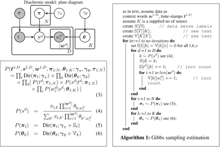
in Figure 1, above which the model is depicted as a plate diagram.
From a generative perspective, theπ1:N andθ1:K are generated fromN andK samplings and then
used forallDdata items. In actual data, the time-stamps and words are known, so for any fixed setting of γπ,γθ there is a defined posterior distribution on s1:D,π1:N,θ1:K. A Gibbs sampling algorithm
(Gelfand and Smith, 1990) can be derived, generating a large set of samples of this(D+N +K)-tuple, representative of this posterior, from whichmeanvalues of the model parametersπ1:N andθ1:K can be
derived. To arrive at the Gibbs sampler, sampling distributions for sd,πt andθk are needed, in each
case conditioned on allotherparts of the sample tuple. The formulae for these sampling distributions are shown as (4 – 6) in Figure 1 : in these formulaeSt[k]is the number of data items with time-stampt
and sampled sensekandVk[v]is the number of times wordvoccurs in data items with sampled sense
k. The derivation of these formulae is relatively straightforward given well-known conjugacy properties of Dirichlet priors – Appendix A gives an outline derivation forπt. The sampling algorithm is given in
pseudo-code in Figure 1.
2.1 Ground truth for semantic neologisms?
Given a large-scale, time-stamped andsense-labeled corpus for a target expressionσ, it would be easy to determine a true emergence date — call itC0 — at which a new sense forσ first departed from zero
frequency (and continued to climb from zero). It has been noted (Lau et al., 2012; Cook et al., 2013) that such reference corpora do not exist, thus posing the question of what can serve as ground truth instead.
Diachronic model: plate diagram
θ π
Sd
γπ
wd i
γθ
t
τ
|wd|
D K
N
P(t1:D,s1:D,w1:D,π1:N,θ1:K;γ
π,γθ,τ1:N) =QtDir(πt;γπ)×QkDir(θk;γθ)
×Qd[P(td;τ
1:N)×P(sd|td;π1:N) ×QiP(wd
i|sd;θ1:K) ]
(3)
P(sd) = πt,k Q|wd|
i=1 θk,wd i
P
k0πt,k0Q|i=1wd|θk0,wd i
(4)
P(πt) = Dir(πt;γπ+St) (5)
P(θk) = Dir(θk;γθ+Vk) (6)
as in text, assume data as
context wordsw1:D, time-stampst1:D
assumeKis a supplied no of senses
createS[D]; // data sense labels
createS[T][K]; // see text
createV[K][V]; // see text
foritr:=1 to no-iterationsdo
setS[t][k] =V[k][v] = 0for allt,k,v ford:=1 to Ddo
k∼P(sd)see (4);
S[d] =k;
S[td][k] += 1; // incr count fori:=1 tolen(wd)do
V[k][wd
i] += 1; // incr
count
end end
fort:=1 to Ndo
πt∼P(πt)see (5);
end
fork:=1 to Kdo
θk∼P(θk)see (6);
end end
[image:3.595.78.523.65.363.2]Algorithm 1:Gibbs sampling estimation
Figure 1: From top left in anti-clockwise shows: plate digram for diachronic model, Gibbs sampler updates, and pseudo-code for Gibbs sampler
thisDi
0. The time resolution of this is low and the subtle criteria involved in inclusion decisions make it
a non-ideal approximation ofC0(Sheidlower, 1995; Simpson, 2000; Barnhart, 2007). Some researchers
(Lau et al., 2012) use this, though we will not. More accessibly, an historically oriented dictionary (eg. the Oxford English Dictionary (OED)) strives to include the earliest known use of a word in a particular sense — the so-calledearliest citation. If we call thisDc
0, it seems to makes sense to useD0cas alower
bound onC0, and we will do this.Dc0represents a first use, which might be followed by a long interlude
before the usage is really taken up: the experiments in Section 3.2 will highlight examples of this. We propose to use a different technique to establishC0more precisely. If there are words which it is
intuitive to expect in the vicinity of a target wordσin the novel sense, and not in other senses, then by consulting a time-stamped corpus one should see the probability of finding these words inσ’s context start to climb at a particular time. For example,mousehas come to have a ‘computer pointing device’ sense, and in this usage it is intuitive to expect words likeclick,button,pointeranddragin it’s context. For any wordwand targetσletPt(w|σ)bew’s probability of occurring inσ’s context in data from time
t, and lettrackσ(w)to be the sequence these values. If whentrackmouse(w) is plotted for the above
words, they all show a sharp increase at thesametime point, this is good evidence that this isC0– the
right-hand plot in Figure 3(a) is an example of this. This combines co-occurrence intuitions with corpus data, and doesnotrely on somewhat unreliable speaker intuitions of recency. To forestall any possible confusion, this procedure of inspecting the probabilities of words thought especially associated with a particular sense isnotbeing advanced as a proposed unsupervised algorithm to locate sense emergences. It is advanced as a way to establish a ground-truth concerning emergence by which to evaluate our proposed unsupervised algorithm.
3 Data and Experiments
Target Years Lines New sense OED Tracks GS-Date <10%
mouse 1950-2008 910k computer pointing device 1965 1983 1982 yes
gay 1900-2008 1253k homosexual person 1922 1966 1969 yes
strike 1800-2008 5052k industrial action 1810 1880 1866 yes
bit 1920-2008 7393k basic unit of information 1948 1965 1954 no
paste 1950-2008 318k duplicate text in computer edit 1975 1982 1981 yes compile 1950-2008 689k transform to machine code 1952 1966 1971 yes
surf 1950-2008 182k exploring internet 1992 1994 1993 yes
boot 1920-2008 1285k computer start up 1980 1980 1984 yes
rock 1920-2008 4136k genre of music 1956 1965 1965 yes
stoned 1930-2008 79k under drug influence 1952 1970 1979 no
Target Years Lines
ostensible 1800-2008 130k present 1850-2008 56333k
cinema 1950-2008 305k
promotion 1930-2008 1681k theatre 1950-2008 1125k
play 1950-2008 13726k
plant 1900-2008 8175k
[image:4.595.73.527.63.155.2]spirit 1930-2008 11573k
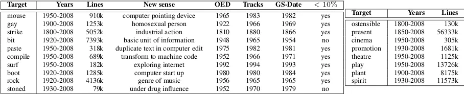
Table 1: Google 5 gram dataset - the left table provides the information for targets that are neologisms while the right one has the targets for non-neologisms – see text for explanation of columns
1≤n≤5: so for any givenn-gram,x, and any year,t, it gives the total frequency2of occurrences ofx across all books dated to yeart. For a given target wordσwe use the subset of all the data consisting of the5-grams that containσ; we use the 5-grams as they provide most context around the targetσ. For the targetmousethe following is an example of a line of data from the corpus
Enter or click the mouse 1990 9 7
The first of the final three numbers is a year. The penultimate number is the number of occurrences of the 5-gram in all publications from that year – this is the significant count data for the algorithm. The final number is the number of publications from the year that contain the 5-gram, which is not significant for the algorithm.
For the experiments reported in Section 3.2 two sets of targets were chosen. The first set{mouse, gay, strike, bit, paste, compile, surf, boot, rock, stoned}are words which, relative to particular time periods, are known to exhibit sense emergence. The second set{ostensible, present, cinema, promotion, theatre, play, plant, spirit}are words which, relative to particular time periods, are thoughtnotto exhibit sense emergence. Following Lau et al. (2012) the idea is that these should provide both positive and negative tests for the algorithm. Table 1 lists the targets. For each target, the ‘Years’ and ‘Lines’ columns give the range of years used and the total number of 5-gram lines of data for that year-range. For the positive targets the ‘New sense’ column gives an indication of the emergent sense and the next two columns give two kinds of reference dating information – see Section 2.1 – the OED first citation date and the ‘tracks’-based date that is apparent from ‘tracks’ plots for words that are intuitively associated with the emergent sense (the right-hand plot in Figure 3(a) is an example). The ‘GS date’ column gives the emergence date inferred when the inference algorithm was run and will be discussed further in Section 3.2.
Before describing the experiments it is necessary to emphasize the Google n-gram data-set is best thought of as a frequency table giving per-year counts associated with 5-gram types. It is not really a corpus of text tokens. For brevity Algorithm 1 was formulated assuming that each data item represented a single target token. Any original publication token of a target σ could have contributed to several different 5-gramtypecounts (up to 5) but the data-set makes it impossible to know to what extent this is so. We therefore effectively treat each 5-gram data entrydlisted with frequency ofndas if it derives
from nd tokens of σ which contributed to no other 5-gram counts. This leads to changing the count
increment operations in Algorithm 1 to addndrather than 1, that is,S[t][k]+=ndandV[k][w]+=nd.
For all of the experiments sampling is done according to Algorithm 1, for 10000 iterations, with the first 1000 discarded as ‘burn-in’ samples and then means are determined for the model parametersπ1:N
(sense-given-year) andθ1:K (word-given-sense) from the sampled values. The parametersγπ andγθ
of the Dirichlet priors are set to have 1 in all positions to make them non-informative priors so uniform over all possibleπtandθk. The sampler is initialised with valuesπ1:N andθ1:K in the following way.
LetPcorpbe the observable corpus word probabilities inw1:D. Eachθkis set to(1−α)Pcorp+αPran,
wherePranis a random word distribution andαis a mixing proportion, here set to10−1. Theπtare set
to some shared set of sense probabilities. Thus initially the word distributions for each sensekare almost identical, and the sense distributions are the same at all times, so far from the neologism situation.
The procedure was implemented in C++. To obtain the code or data see www.scss.tcd.ie/
Martin.Emms/SenseDynamics.
3.1 Experiments with ‘pseudo’-neologisms
The ‘pseudo-word’ technique was introduced in Sch¨utze (1998) as a possible means to test unsupervised word-sense discrimination. It can be given a diachronic twist to furnish what might be called ‘ pseudo-neologisms’ in the following way. Relative to some period of time select two words, σ1 andσ2, both
unambiguous, withσ1in use throughout the time period, but withσ2first emerging at some point,te, in
the period. If the 5-grams forσ1 andσ2 are then all treated as examples of the fake word ‘σ1-σ2’ this
functions as an artificalsemanticneologism, manifestingσ2’s sense only fromteonwards. Furthermore,
if we sayft(σi) gives the true empirical probability of targetσi in pooledσ1,σ2 data for timet, then
ideally the outcome of inference when run forK= 2should be that for eachk, the trajectory of theπt[k]
values is very similar to that for one of theft(σi). We tested this, for the time-period 1850–2008, with ‘ostensible’ forσ1 (present throughout), and ‘supermarket’, ‘genocide’ and ‘byte’ as possibilities forσ2
(which emerged as new words over this time frame) and indeed obtained the desired correspondence between inferredπt[k]and empiricalft(σi)trajectories – Figure 2 shows the outcomes for the first two. For the first case the succession of πt[1] values matches closely the succession of ft(‘supermarket’)
values, and in the second case theπt[0]values match theft(‘genocide’) values. To get an insight into
the inferredθkvalues, we definedgist(S)to be the top 20 words when ranked according to the ratio of
P(w|S)toPcorp(w). For the apparently neologistic senseS, Figure 2 also showsgist(S)and it can be seen that these sets of words seem very consistent with relevant parts of the pseudo-neologisms.
Thus on these pseudo-neologisms, the proposed model and algorithm has been successful, identifying an emerging ‘sense’ in an unsupervised fashion. Moving on from this first test of the algorithm, the next section considers outcomes on authentic words.
(a)ostensible-supermarket (inferred and empirical)
1850 1900 1950 2000
0.0
0.2
0.4
0.6
0.8
1.0
Year
Sense Prop
sense 0 sense 1
1850 1900 1950 2000
0.0
0.2
0.4
0.6
0.8
1.0
Year
Probs
supermarket
ostensible
(b)ostensible-genocide (inferred and empirical)
1850 1900 1950 2000
0.0
0.2
0.4
0.6
0.8
1.0
Year
Sense Prop
sense 0 sense 1
1850 1900 1950 2000
0.0
0.2
0.4
0.6
0.8
1.0
Year
Probs
genocide
ostensible
gist(sense 1) :at, a, ., local, END , in, go, your, chain, checkout,
shelves, from, or, line,you, store, buy, shopping gist(sense 0):1994, Nazi, cultural, Armenian, cleansing, ethnic, Jews, term, dur-crimes, against, Rwanda, commit, humanity, in, war,
[image:5.595.82.522.396.537.2]ing, crime, victims, slavery
Figure 2: For (a-b), the left-hand plots show the inferredπt[k]sense parameters for a pseudo-neologism
σ1-σ2, and right-hand plot shows the knownσ1andσ2proportions. Below the plots are ‘gist(S)’ words
associated to the apparent neologism sense – see text.
3.2 Experiments with genuine neologisms
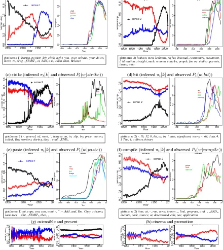
Table 1 listed both targets expected to show sense emergence and targets expected to not show sense emergence. For several of the sense emergence targets, Figure 3(a-d) depicts various aspects of the outcomes. In each case the leftmost plot for a targetσshows for eachkthe succession of inferredπt[k]
values – the sense-given-year values – plotted as a solid line3; the rightmost plot in each case is a ‘tracks’ plot (see Section 2.1), showing for some collection of words considered to be associated with the novel sense the succession of their probabilities of occuring in n-grams for the targetσ,Pt(w|σ). These are
the basis for the ‘tracks’ column in Table 1.
mouseFigure 3(a): The algorithm was run looking for 3 sense variants on data between 1950 and 2008. The blue line for theπt[1]sequence in the left-hand plot shows a neologistic pattern, starting near0and
(a) mouse (inferredπt[k]and observedPt(w|mouse))
1950 1970 1990 2010
0.0 0.2 0.4 0.6 0.8 Year Sense Prop mouse sense 1
1950 1960 1970 1980 1990 2000 2010
0.0 0.2 0.4 0.6 0.8 mouse Year w ord probs click button pointer drag
gist(sense 1)button, pointer, left, click, right, you, over, release, your, down, move, to, drag, START , is, hold, use, when, then, Release
(b) gay (inferredπt[k]and observedPt(w|gay))
1900 1920 1940 1960 1980 2000
0.0 0.2 0.4 0.6 0.8 Year Sense Prop gay sense 2
1900 1920 1940 1960 1980 2000
0.0 0.2 0.4 0.6 0.8 gay Year w ord probs community men rights lesbian
gist(sense 2)lesbian, men, lesbians, rights, bisexual, community, movement, /, liberation, straight, male, women, couples, people, for, or, studies, parents, issues, who
(c) strike (inferredπt[k]and observedPt(w|strike))
1800 1850 1900 1950 2000
0.0 0.1 0.2 0.3 0.4 0.5 0.6 Year Sense Prop strike sense 2
1800 1850 1900 1950 2000
0.0 0.2 0.4 0.6 0.8 strike Year w ord probs union coal miners
gist(sense 2)-, general, of, went, ’, hunger, on, in, slip, by, price, miners, called, The, workers, during, day, ., coal, END
(d) bit (inferredπt[k]and observedPt(w|bit))
1920 1940 1960 1980 2000
0.0 0.1 0.2 0.3 0.4 0.5 Year Sense Prop bit sense 2
1920 1940 1960 1980 2000
0.0 0.2 0.4 0.6 0.8 bit Year w ord probs X8 X32 X64 memory
gist(sense 2)-, 16, 32, 8, bit, as, by, (, rate, significant, every, –, 64, data, 4, ), The, 1, address, binary
(e) paste (inferredπt[k]and observedPt(w|paste))
19500.0 1970 1990 2010
0.2 0.4 0.6 0.8 1.0 Year Sense Prop paste sense 1
1950 1960 1970 1980 1990 2000 2010
0.0 0.2 0.4 0.6 0.8 1.0 paste Year w ord probs cut copy text image clipboard
gist(sense 1)cut, copy, you, can, want, -, ”, –, Add, and, You, Copy, scissors, tomatoes, ’, Cut, START , then, ,
(f) compile (inferredπt[k]and observedPt(w|compile))
1950 1970 1990 2010
0.0 0.1 0.2 0.3 0.4 0.5 0.6 Year Sense Prop compile sense 2
1950 1960 1970 1980 1990 2000 2010
0.0 0.2 0.4 0.6 0.8 compile Year w ord probs errors fixed detected
gist(sense 2)time, at, -, run, error, known, ,, link, program, and, ., END , execute, code, source, or, determined, edit, not, application
(g) ostensible and present
1800 1850 1900 1950 2000
0.2 0.5 0.8 Year Sense Prop ostensible
1850 1900 1950 2000
0.15
0.30
0.45
Year
Sense Prop
present (h) cinema and promotion
19500.35 1970 1990 2010
0.50
0.65
Year
Sense Prop
cinema
1940 1960 1980 2000
[image:6.595.79.519.77.570.2]0.35 0.50 0.65 Year Sense Prop promotion
Figure 3: For (a-f), the left-hand plot shows the inferredπt[k]sense parameters, with the sense number
Sof the potential neologism labeled; the right-hand plot show probability ‘tracks’ for some words intu-itively associated with the neologism (see text for further details). The box below the plots has top 20
gist(S)words for the neologism senseS. (g-h) show the inferredπt[k]sense parameters for negative targets
departing from 0 around1983. The ‘tracks’ plot also shows that several words intuitively associated with the neologistic sense, also drastically increase their probability conditioned onmousearound the same time. The ‘GS-date’ column of Table 1 gives the timet, if any, in aπt[k]sequence where it appears to
depart from, and continues to climb from, zero. The ‘<10%’ column records whether this agrees with the tracks-based date to within10%of the time-span considered – which it does in this case. Notably in this case, the GS-based emergence date, though close to the tracks-based date, is more than 20 years
date at which this use of the termmousedeparted and continued to climb from zero in the n-grams books based data is substantially later. We take this to illustrate why simply taking the OED first citation date,
Dc
0, as a gold standard for the true corpus emergence date,C0, would be a mistake4. The box below the
plots in Figure 3(a) tries to give some insight into the estimatedθ1 parameter concerning
word-given-sense probabilities by showing the words belonging togist(1)(see definition in section 3.1). They seem mostly consistent with the ‘pointing device’ sense.
gayFigure 3(b): In this case the procedure was run on data from 1900 to 2008, for 3 senses. In the left-hand plot the black line, for theπt[2]sequence, shows sense emergence, appearing to depart from
near zero first around 1969. The ‘tracks’ plots to the right seem to increase around around 1966. The OED first citation date of 1922 predates both considerably. The ‘gist’ words forS = 2also seem mostly consistent the ‘homosexual’ sense.
Similar to mouseandgay, the detailed outcomes forstrike, bit, paste, compile are shown in figures (c - f) with the procedures run on data for 3 senses. For space reasons, these details are not shown for
boot, surf, strike, rockandstonedbut Table 1 summarizes all outcomes: in each case the inferred date was later than the OED first citation date, and in all cases close to the tracks-based date, just missing the
10%margin in two cases.
Turning to the words which werenotexpected to exhibit an emergent sense, Figure 3(g-h) shows the plots of the inferred πt[k]sequences for the targets ostensible, present, cinema andpromotion. None show a clear neologistic pattern, in line with expectations. Though the details are not shown in Figure 3 the same kind of outcome was found for the other negative targets listed in Table 1.
The value ofK varied somewhat between the experiments. That the number of senses possessed by the different targets varies is somewhat to be expected and in some cases where a neologistic trend was less clear withnsenses, it became clearer withn+ 1. The automatic setting of this parameter remains an area for future work.
4 Comparisons to related work and conclusions
We have looked at the detection that a word has acquired the possibility to express a meaning which it could not hitherto (eg. mouseas pointing device). One can also look at senses themselves as changing over time, perhaps widening or narrowing, and there has been prior work addressing this issue (Sagi et al., 2009). We would like to treat this as a separate issue, though drawing a conclusive line between the two is tricky.
Concerning sense emergence specifically, it has to be stressed there is no strict quantitative state-of-the-art, because it is not the case that prior works share the same targets, use the same data, or address in the same way the tricky ground-truth issue (see Section 2.1). Bearing this in mind we have tried to organise the discussion below around major design options and papers that exemplify these.
There have been some proposals concerning sense emergence detectionwithoutmodelling senses at all (Cook and Hirst, 2011; Kim et al., 2014). Though able to detect a difference between corpora from different eras, these systems tend to lack a capacity to pick out instances exemplifying a putative novel sense, which is arguably a desirable feature.
Moving on to systems which do involve some kind of modelling of senses, a noteworthy characteristic of many is that they often apply a WSI algorithm which is time-unaware. One design option is topoolall training data for the WSI phase, then assign likeliest senses to examples, and then to finally check for a correlation with time, such as a sense only being assigned after a particular time. Another design option is toseparatethe data into eras, perform independent WSI on each subset and then seek to consider how the sense representations from each era may (or may not) belinkedto each other.
The poolingdesign option is exemplified in (Lau et al., 2012; Cook et al., 2013; Cook et al., 2014). Their time-unaware WSI system is based on LDA (Blei et al., 2003), and treats theI words of a context as generated fromI topics, and then identifies a target’s sense with the most frequent amongst theI
number of topics is self-determined by the training process. The equating of senses with topics could be questioned (Wang et al., 2015) and also the self-determined sense number in their illustrative examples seems strikingly high (10), with many unintuitive components included. Rather than a year-by-year time-line, their data is time-stamped to just two timeeras,E1 andE2 (eg. in one of their papersE1 is
the late 20th century (BNC) andE2 is2007 (UkWaC)), and so they attempt a much lower resolution
of emergence dating than we do. Their approach to ground-truth on sense emergence was different also, being that using Di
0 (dictionary inclusion date, mentioned in section 2.1), and so has some of
the drawbacks that were noted there. As we did, they had both positive and negative targets. Without a time-line their evaluation cannot be a comparison of true and inferred emergence date and instead they count success as a tendency to place positives above negatives when ranked by a ‘novelty’ score: the max over k of the ratio of E2 to E1 frequency of assigned sense k. They obtain thus a ranking
on their targets: {domain(116.2),worm(68.4), mirror(38.4),guess(16.5),export(13.8), founder(11.0),cinema(9.7),
poster(7.9),racism(2.4),symptom(2.1) }(with positive targets in bold and negative in italics). As a possible
generalisation of this score to a time-line, consider a ‘novelty’ score computed in the following way: from the sequence of πt[k] values, find ‘min’ and ‘max’ values and divide the temporally later value by the temporally earlier one, letting the novelty score be the max overkof this ratio. On our targets this gives a ranking: { stoned(105),strike(5442.7),gay(2791.1),mouse(1485.9),surf(156.7),compile(26.6),bit(10),
rock(7.4),boot(7),ostensible(3.5),plant(1.89),play(1.8),promotion(1.4),cinema(1.3),theatre(1.1),spirit(1)}, separating the positive from the negative targets. Due to the data and target differences it would not make sense to compare these rankings. Earlier work by Rohrdantz et al. (2011) also instantiates thepoolingoption to exploit a time-unaware system. Their system was again LDA-based, their ground-truth approach was alsoDi
0-based and their data was news articles between 1987 and 2007.
Theseparate-then-linkstrategy for deploying time-unaware WSI to nonetheless attempt to detect sense dynamics is exemplified in (Mitra et al., 2014; Mitra et al., 2015). The time-unaware WSI system in this case is a so-called ‘Distributional Thesaurus’ clustering approach (Rychl´y and Kilgarriff, 2007; Biemann and Riedl, 2013), which starting from a word(type) occurrence graph where edges reflect co-occurrence, induces sets of words to represent a sense. Their data set consists of ‘syntactic dependency n-grams’ as produced by Goldberg and Orwant (2013) from the same digitised books as those from which the Google n-gram data is derived. They divide the entire time-line into erasE1. . .E8of ever shortening duration but containing equal amounts of data (eg. E2 = 1909–53,E7 = 2002-05). For a given target,
for each era they run their clustering to induce sense-representing word sets, and then they propose ways to link the clusters forEi,{si
1, . . . sim}to the clusters of later era Ej,{sj1, . . . sjn}. Roughly speaking a
cluster inEj is judged a ‘birth’ (ie. sense emergence) if sufficiently few of its member words belong
to the any of the clusters for the earlier eraEi. In the paper they discuss outcomes concerning apparent
‘births’ when comparing the 1909-1953 and 2002-2005 eras. They do not test with respect to known positive and negative examples. Instead they apply the procedure toallwords, obtain a very large set of candidate ‘births’, apply a relatively complex multi-stage filtering process to this and then on a randomly selected 48 cases from the filtered ‘births’ they find 60% are correct. Their approach to ground-truth concerning sense emergence (cf. Section 2.1) is somewhat varied but essentially was author intuition in (Mitra et al., 2014) and dictionary first citationDc
0 in (Mitra et al., 2015), though as we have noted this
should only serve as lower bound5.
Unlike these proposals, the experiments in this paper concern a model which is nottime-unaware: the model has variables and parameters referring to time. Earlier versions of this idea were discussed in (Emms, 2013; Emms and Jayapal, 2014; Emms and Jayapal, 2015) though differing from the work presented here in number of respects (such as the estimation approach (EM), data used (text snippets via Google custom date search) and the targets considered (multiword expressions)). This aspect of including time explicitly in a probabilistic model seems to have been considered much less often than the above-mentioned essentially time-unaware approaches. The work of Wijaya and Yeniterzi (2011) is one example. They do not propose a sense-emergence detection algorithm per-se but do make some
5Without getting too lost in case-by-case details, it is worth noting that some seem incorrectly judged true ‘births’ relative
analyses on the Google n-gram data to seek indicators of sense change. They sought to apply theTopics Over Timevariant ofLDA(Wang and McCallum, 2006), to do which they somewhat curiously collapse a year’s worth of n-grams for a target into asingle‘document’ for that year. They found for example that forgay, training for 2 topics, there is a switch from a strong preference for one topic to preference for the other around 1970.
The recent work of Frermann and Lapata (2016) is a further example of a time-aware probabilistic model, in fact one having much in common with the model we have been discussing. They, as we have done, consider a generative model in which for a given time t a sense k is chosen, according to some discrete distribution6 πt, and then, again as we have assumed, the context words in w are generated independently of each other. Whereas we have assumed that word choices are conditionally independent of the time t given the sense k, and so have for each sense k a parameter θk of word
probabilities, they donotassume this independence, and so for eachtimetand sensekhave a parameter
θtk of word probabilities. The key further feature of their model is their use of intrinsic Gaussian
Markov Random Fields(iGRMFs) to have priors which control how the distributionsπtandθtkchange
over time: basically there is a precision hyper-parameter κ such that a high κ favours small changes in successive values. For the succession ofθtk values, they setκ to a high value, so that althoughθtk
does not have to be constant over time, only small variation is anticipated by the prior. The succession ofπt values is allowed greater variation. This use of iGMRF-based priors requires in its turn a more
sophisticated Gibbs sampling approach to parameter estimation than that which we have used – which they achieve following ideas of Mimno et al. (2008). From the perspective of their model, our model is more or less what would be arrived at by (i) lettingκforθtk tend to∞, preventing any change of
word-given-sense probabilites in successive times and (ii) lettingκforπttend to 0, allowing arbitrary change
of sense-given-time probabilities. They evaluated their model in a variety of ways, the most comparable of which was to consider particular target words in theCorpus of Historical American English(Davies, 2010) with number of senses set to 10 and a time-resolution of 10-year time spans. As with the other papers already discussed, their use of different targets and a different data-set means again there is not the possibility at the moment of a quantitative comparison. In our work whilst we do not have a prior to encourage smooth change of theπtvalues, nonetheless relatively smooth changeisobtained, and sense
emergence was successively detected in a number of cases, suggesting that for the n-gram data at least, the more complex system of Frermann and Lapata (2016) is not required. It may be of interest in future work to investigate to what extent this is dependent on the data-set used: the data-set they used contains ~100 times fewer occurrences for a given target per time-period compared to the n-gram data-set we have used and it could be that with less data the priors they propose become more necessary.
In conclusion we have proposed a simple generative model, with aP(S|Y)term for time-dependent sense likelihood, and ap(W|S)term expressing that the context words are independent of time given the target’s sense. The fact that intuitive outcomes were obtained on our pseudo-neologisms, and on some authentic cases of sense emergence and non-emergence is indicative at least that the model’s assumptions are tolerable. It remains for future work involving further targets to test the limits of these assumptions. Amongst several possibiities for further investigation it would be of interest to reformulate the model to refer not just to plain words but rather to syntactic annotations, as well as to consider data sources representing other and more recent text types, such as social media posts.
Appendix A. Derivation of sampling formula forπt
For the sampling formula for πt we need the conditional probability
P(πt|π−(t),s1:D,w1:D,t1:D,τ1:N,θ1:K;γπ,γθ), where indexing by −(t) is meant to indicate
consideration of all indicesexceptt. This conditional probability is given by
P(πt,π−(t),s1:D,w1:D,t1:D,τ1:N,θ1:K;γπ,γθ) R
πtP(πt,π−(t),s1:D,w1:D,t1:D,τ1:N,θ1:K;γπ,γθ) Recalling the model formula (3) given in Figure 1 the numerator in this fraction is
6Adapting their notation to make things as comparable as possible: they haveΦtrather thanπ
Y
d
τtd×πtd,sd×
|Ywd|
i=1
θsd,wd i
×Dir(πt;γπ)×Y
−(t)
Dir(π−(t);γπ)× Y
1:K
Dir(θk;γθ)
and the denominator differs only by the the integral overπt. πtis involved in the Dir(πt;γπ)term and
in those parts of the product fordwhere you havetd=t. Because of this most terms in the denominator
can be taken outside the scope of the integral and then cancel with corresponding terms in the numerator. Because of this, the fraction can be written
Q
d:td=t[πt,sd]×Dir(πt;γπ)
R
πt
hQ
d:td=t[πt,sd]×Dir(πt;γπ)
i
In the data items {d : td = t} a variety of sense values have been sampled and the numerator can
instead be expressed usingSt,k, which counts the sampled sense values (see Section 2). Re-expressing
the numerator in this way and using the definition of the Dirichlet (Heinrich, 2005), we get
Y
k
πSt,k
t,k × β(γ1 π)
Y
k
πγπ[k]−1
t,k = β(γ1 π)
Y
k
πSt,k+γπ[k]−1
t,k
Hence the fraction can be written
Q
kπSt,kt,k+γπ[k]−1 R
πt[
Q
kπSt,kt,k+γπ[k]−1]
= β(S 1 t+γπ)
Y
k
πSt,k+γπ[k]−1
t,k
where the last step uses the fact that in any Dirichlet Dir(x1:K;α1:K) = β(α11:K)
QK
k=1xαkk−1, the
‘normalizing’ constantβ(α1:K)is the integral of the main product term. Hence we finally obtain
P(πt|π−(t),s1:D,w1:D,t1:D,θ1:K;γπ,γθ) =Dir(πt;γπ+St)
which is the sampling formula given earlier as (6). The derivation of the sampling formula forθk is
similar, and that for the discretesdis straightforward. Acknowledgments
This research is supported by Science Foundation Ireland through the CNGL Programme (Grant 12/CE/I2267) in the ADAPT Centre (www.adaptcentre.ie) at Trinity College Dublin.
References
David Barnhart. 2007. A calculus for new words. Dictionary, 28:132–138.
Chris Biemann and Martin Riedl. 2013. Text: Now in 2d! a framework for lexical expansion with contextual
similarity. Journal of Language Modelling, 1(1):55–95, Apr.
David M. Blei, Andrew Y. Ng, and Michael I. Jordan. 2003. Latent dirichlet allocation. InJournal of Machine
Learning Research, volume 3, pages 993–1022,, March.
Paul Cook and Graeme Hirst. 2011. Automatic identification of words with novel but infrequent senses. In
Proceedings of the 25th Pacific Asia Conference on Language Information and Computation (PACLIC 25),
pages 265–274, Singapore, December.
Paul Cook, Jey Han Lau, Michael Rundell, Diana McCarthy, and Timothy Baldwin. 2013. A lexicographic
appraisal of an automatic approach for detecting new word senses. InProceedings of eLex 2013.
Paul Cook, Jey Han Lau, Diana McCarthy, and Timothy Baldwin. 2014. Novel word-sense identification. In
Pro-ceedings of COLING 2014, the 25th International Conference on Computational Linguistics, page 1624–1635.
Mark Davies. 2010. The corpus of historical american english: 400 million words, 1810-2009. available online at
http://corpus.byu.edu/coha.
Martin Emms and Arun Jayapal. 2014. Detecting change and emergence for multiword expressions. In
Proceed-ings of the 10th Workshop on Multiword Expressions (MWE), pages 89–93, Gothenburg, Sweden. Association
for Computational Linguistics.
Martin Emms and Arun Jayapal. 2015. An unsupervised em method to infer time variation in sense probabilities.
InICON 2015: 12th International Conference on Natural Language Processing, pages 266–271, Trivandrum,
India, December.
Martin Emms. 2013. Dynamic EM in neologism evolution. In Hujun Yin, Ke Tang, Yang Gao, Frank Klawonn,
Minho Lee, Thomas Weise, Bin Li, and Xin Yao, editors,Proceedings of IDEAL 2013, volume 8206 ofLecture
Notes in Computer Science, pages 286–293. Springer.
Lea Frermann and Mirella Lapata. 2016. A Bayesian model of diachronic meaning change. Transactions of the
Association for Computational Linguistics, 4:31–45.
Alan E. Gelfand and Adrian F. M. Smith. 1990. Sampling-based approaches to calculating marginal densities.
Journal of the American Statistical Association, 85(410):398–409, jun.
Yoav Goldberg and Jon Orwant. 2013. A dataset of syntactic-ngrams over time from a very large corpus of english
books. InSecond Joint Conference on Lexical and Computational Semantics (*SEM), Volume 1: Proceedings
of the Main Conference and the Shared Task: Semantic Textual Similarity, pages 241–247, Atlanta, Georgia,
USA, June. Association for Computational Linguistics.
Gregor Heinrich. 2005. Parameter estimation for text analysis. Technical report, Fraunhofer Computer Graphics Institute.
Yoon Kim, Yi-I. Chiu, Kentaro Hanaki, Darshan Hegde, and Slav Petrov. 2014. Temporal analysis of language
through neural language models. CoRR, abs/1405.3515.
Jey Han Lau, Paul Cook, Diana McCarthy, David Newman, and Timothy Baldwin. 2012. Word sense induction
for novel sense detection. InProceedings of the 13th Conference of the European Chapter of the Association
for Computational Linguistics (EACL 2012), pages 591–601, Avignon, France, April.
Jean-Baptiste Michel, Yuan Kui Shen, Aviva Presser Aiden, Adrian Veres, Matthew K. Gray, The Google Books Team, Joseph P. Pickett, Dale Hoiberg, Dan Clancy, Peter Norvig, Jon Orwant, Steven Pinker, Martin A. Nowak,
and Erez Lieberman Aiden. 2011. Quantitative analysis of culture using millions of digitized books. Science,
331(6014):176–182.
David Mimno, Hanna Wallach, and Andrew McCallum. 2008. Gibbs sampling for logistic normal topic models
with graph-based priors. InNIPS Workshop on Analyzing Graphs.
Sunny Mitra, Ritwik Mitra, Martin Riedl, Chris Biemann, Animesh Mukherjee, and Pawan Goyal. 2014. That’s
sick dude!: Automatic identification of word sense change across different timescales. InProceedings of the
52nd Annual Meeting of the Association for Computational Linguistics, page 1020–1029. Association for
Com-putational Linguistics, June.
Sunny Mitra, Ritwik Mitra, Suman Kalyan Maity, Martin Riedl, Chris Biemann, Pawan Goyal, and Animesh Mukherjee. 2015. An automatic approach to identify word sense changes in text media across timescales.
Natural Language Engineering, 21(5):773–798.
Christian Rohrdantz, Annette Hautli, Thomas Mayer, Miriam Butt, Daniel A. Keim, and Frans Plank. 2011.
Towards tracking semantic change by visual analytics. InProceedings of the 49th Annual Meeting of the
Asso-ciation for Computational Linguistics, pages 305–310. ACL, June.
Pavel Rychl´y and Adam Kilgarriff. 2007. An efficient algorithm for building a distributional thesaurus (and other
sketch engine developments). In Proceedings of the 45th Annual Meeting of the ACL on Interactive Poster
and Demonstration Sessions, ACL ’07, pages 41–44, Stroudsburg, PA, USA. Association for Computational
Linguistics.
Eyal Sagi, Stefan Kaufmann, and Brady Clark. 2009. Semantic density analysis: Comparing word meaning across
time and phonetic space. InProceedings of the EACL 2009 Workshop on GEMS: GEometical Models of Natural
Language Semantics, page 104–111. Association for Computational Linguistics, March.
Jesse T. Sheidlower. 1995. Principles for the inclusion of new words in college dictionaries. Dictionaries, 16:32– 43.
John Simpson. 2000. Preface to the third edition of the oed. public.oed.com/the-oed-today/
preface-to-the-third-edition-of-the-oed.
Yee Whye Teh, Michael I. Jordan, Matthew J. Beal, and David M. Blei. 2004. Hierarchical dirichlet processes.
Journal of the American Statistical Association, 101.
Jean Tournier. 1985.Introduction descriptive `a la lexicog´en´etique de l’anglais contemporain. Champion-Slatkine.
Xuerui Wang and Andrew McCallum. 2006. Topics over time: A non-markov continuous-time model of topical
trends. InProceedings of the 12th ACM SIGKDD International Conference on Knowledge Discovery and Data
Mining, KDD ’06, pages 424–433, New York, NY, USA. ACM.
Jing Wang, Mohit Bansal, Kevin Gimpel, Brian D. Ziebart, and Clement T. Yu. 2015. A sense-topic model
for word sense induction with unsupervised data enrichment. In Hwee Tou Ng, editor, Transactions of the
Association for Computational Linguistics, page 59–71. Association for Computational Linguistics, January. Derry Tanti Wijaya and Reyyan Yeniterzi. 2011. Understanding semantic change of words over centuries. In
Proceedings of the 2011 International Workshop on DETecting and Exploiting Cultural diversiTy on the Social
![Figure 2: For (a-b), the left-hand plots show the inferred π 1 t [ k ] sense parameters for a pseudo-neologismσ - 2 , and right-hand plot shows the known σ 1 and σ 2 proportions](https://thumb-us.123doks.com/thumbv2/123dok_us/770271.1089587/5.595.82.522.396.537/figure-inferred-parameters-pseudo-neologisms-right-known-proportions.webp)