VaR methods for linear instruments

(1)

VaR methods for linear instruments

(2)

Title: VaR methods for linear instruments Author: Birgir Viðarsson

Instructor: Dr. Freyr Harðarson. Risk Management, Landsbanki

Examiner: Dr. Henrik Johansson. Department of Fire Safety Engineering and Systems Safety, Lund University

Report nr.: 5268 ISSN: 1402-3504

ISRN: LUTVDG/TVBB5268SE

Keywords

VaR, Volatility, Covariance, GARCH, EWMA, Univariate, Multivariate, Market risk, Financial time series

Abstract

In this thesis various Value-at-Risk models are compared and evaluated to-wards nding the optimal model for the bank's trading book. The focus is on linear instruments (stocks, indicies and currency) and real market data, both domestic and foreign, is used for the calculations. I nd that the GARCH(1,1) based model outperforms other models in volatility estimation and should thus be a wise choice when volatility estimation is needed, but GARCH based methods become rather complex for a multivariate covari-ance estimation. Therefore a mixture of simpler models such as EWMA is needed for making rational estimates.

c

Copyright: Brandteknik och Riskhantering, Lunds tekniska högskola,

Lunds universitet, Lund 2008.

Brandteknik och Riskhantering Department of Fire Safety Lunds tekniska högskola Engineering and Systems Safety

Lunds universitet Lund University

Box 118 P.O. Box 118

221 00 Lund SE-221 00 Lund

Sweden

[email protected] [email protected] http://www.brand.lth.se http://www.brand.lth.se/english

(3)

(4)

(5)

In the last decades the growth in nancial markets has been enormous. Global trading is easier then ever and business with all kinds of nancial instrument such as stocks and bonds and their derivatives is common. Usu-ally the aim with all trades is to save or gain money one way or another, but with all trades there exist as well the risk that the trade will not be protable and result in a nancial loss. This risk that leads to nancial loss can be regarded as nancial risk. One of the main category of nancial risk is market risk which is the risk that market uctuations will lead to nan-cial loss. For nannan-cial institutions who have large amount of their assets in nancial instrument (traded on markets), market risk can have great impact on their performance and therefore essential to quantify.

In this thesis the goal is to quantify market risk and for that cause use the term Value-at-Risk (VaR), which is commonly used among nancial institu-tions. The term VaR is dened as the amount X that you are α% certain

of not losing more than the following N days. More general, VaR gives a kind of worst case scenario at preferred level of probability (α) and time pe-riod (N-days). There are various ways and techniques for calculating VaR, all with their pros and cons, and generally depended on presumptions. In this thesis the focus is on linear instruments, such as equity and currency, and for that sake the main categorize of calculating VaR are parametric and non-parametric approaches. VaR is also used in regulatory terms. The Basel Committee, which is a international banking supervisor, uses VaR to stip-ulate the minimum amount of regulatory capital that nancial institution must have available at all times. This is done to prevent nancial crisis and possible bankruptcy due to unforeseen market movements, credit defaults or any other risk faced by the nancial institution. Both parametric and non-parametric methods are used to calculate VaR for real market data, with the goal of nding the method that suits the bank's trading book the best while fullling regulations set by the Basel Committee.

(6)

Introduction

As pointed out by Kaplan and Garrick (1981) quantitative risk can be dened as combination of scenario, probability and a consequence. It is necessary to evaluate all these parts to get a relative and rational estimate of risk. More general in risk assessment and risk management we want to answer the question; What can go wrong, how likely is it and what will be the consequences. The main elds of risk assessment can be separated into 5 categories; Safety risk, Health risk, Ecological and Environmental risk, Public welfare risk and Financial risk (Kolluru, 1995).

Financial risk can be thought of as any risk concerned with nancial loss due to some random changes in underlying risk factors (stock, currency, derivatives, interest rate etc.) and can furthermore be categorized into three main level of concerns; Market risk (due to movements in market factors), Credit risk (the risk that a person or an organization will not fulll his/her obligations) and Operational risk (risk of loss because of systematic failures) (Dowd, 1998). Methods for measuring and evaluating nancial risk are many and depend on what is of interest to examine. Just for market risk there are numerous of ways. For options and derivatives examining `the greeks' might by a good choice, stress testing might by good for worst case scenario anal-ysis while Value-at-Risk (VaR) could give a universal risk measure for the exposed market risk. In this thesis I will concentrate on VaR for measuring market risk1_.

In the last 50 years there has been enormous growth in trading worldwide, for example the New York Stock Exchange has grown from $4 million in

1961 to $1.6 trillion2 in 2005. This growth and the massive increase of

new instruments (all kinds of derivatives, swaps, CDO's (collateralized debt obligation) and so on) has invoked more need for good risk management in

1_{This was proposed by Landsbanki bank} 2_{One trillion equals million millions}₍₁₀12

(9)

the nancial sector. Managing risk improves the value of the company and can avoid major nancial disaster such as Orange County (1994), Barings Bank (1995), Enron (2001), WorldCom (2002) and Sociètè Générale (2008) which have all been related to poor risk management.

1.1 Aim and purpose

The aim of the thesis is to evaluate dierent methods for calculating VaR for bank's trading book, where the goal is to minimize VaR while fullling regulatory requirements. The focus will be on linear instruments (such as equity and currency) and actual market data will be used for the evaluation, both domestic and foreign (Icelandic and Swedish).

VaR estimation can be categorized into three main categories; parametric methods, non-parametric methods and Monte Carlo simulation methods. Both parametric and non-parametric approaches will be used to calculate VaR for the market data and compared with critical judgment to-wards obtaining the optimal VaR method for the bank's trading book. Monte Carlo methods are mostly used on non-linear nancial instruments and will therefore not be the topic of this thesis.

1.2 What is VaR?

You are responsible for managing your company's foreign ex-change positions. Your boss, or your boss's boss, has been read-ing about derivatives losses suered by other companies, and wants to know just how much market risk the company is tak-ing. What do you say?

(10)

1.2 WHAT IS VAR? 3

to hedge, but they understand that this statement is vacuous. They know that the word `hedge' is so ill-dened and exible that virtually any transaction can be characterized as a hedge. So what do you say? (Linsmeier and Pearson, 1996)

Value at Risk (VaR) is an attempt to give a relatively simple measure of nancial risk (not only market risk) with a single number answering the question `how bad can things get?' (Dowd, 2005). VaR could thus be a fair attempt to answer the question in the example above. The statement we wan't to make with VaR is:

We are α percent certain to lose not more thanX much money in the following N days.

The amount X is a loss due to market movements and could be for a sin-gle asset or a portfolio (see section 2.2). The amount X is function of two variables, the condence level α and time period, usually given in N days. The calculation of VaR is thus based on the probability of changes in asset or the portfolio value over the next N days. To be more mathematical VaR is the quantile corresponding to the (1 - α) of the return distribution, so if we setp= 1−αand callqp thep-th quantile ofα, then VaR can be dened

as; VaRα%=−qp for specied condence level and period. Meaning that we

can beα certain to not lose more than VaR in that period (see gure 1.1)

Figure 1.1: VaR at α% condence level for some imaginary prot/loss series,

as-suming normality

(11)

a company is interested in knowing their market risk status and especially what the1−α worst case would be. Then VaRα% would give a estimate of

the loss that would not be exceeded α percent of the time. Likewise, losses larger then VaRα% happen only (1 -α)% of the time. This VaRα% is equal

to the boundaries between the blue and white area on gure 1.1.

The reason for VaR's popularity, as a denition of risk, is its simplicity in interpretation. It is relatively easy to understand, has the unit of the mea-sure (i.e. euro, SEK, ISK)3_{, it is probabilistic (concerned with probability), it}

can be used for any type of positions (bond, stock, currency, derivatives etc.) and portfolios (meaning that it will aggregate many sub-positions into one measure) and it is holistic (meaning that takes into account all underlying risk factors) (Dowd, 2005). VaR is also used in regulatory terms. Financial institutions are required to have some minimum regulatory capital available at all times for safety reasons and with the Basel accord4_{, nancial}

insti-tution were allowed to base this minimum capital partly on their own VaR estimates. This is known as the internal approach, see section 5.1.1.

1.3 Data

In the thesis I will examine four stocks, two indices, two portfolios and one currency pair. Portfolio 1 will be made of equal shares (25%) in all four

stocks, 25% LAIS, 25% MARL, 25% NDA and 25% ERIC and Portfolio 2

will consist stocks in the following ratios;50%LAIS,30%MARL,10%NDA

and10% ERIC, see 1.1.

Name Ticker Description Landsbankinn LAIS Icelandic bank

Marel MARL Icelandic food processing company

OMX Iceland 15 ISXI15 Index consisting of 15 Icelandic companies Nordea NDA Swedish bank

Ericsson ERIC Swedish tele & datacommunication company OMX OMX Index consisting of 30 Swedish companies Portfolio 1 - Equal share portfolio

Portfolio 2 - 50% LAIS, 30% MARL, 10% NDA and 10% ERIC USD/ISK USDISK USA dollars to Icelandic króna

Table 1.1: The time series used for calculation

3_{In the thesis I will though use percentage for the sake of comparison, see section 5.1} 4_{Banking supervision accords (recommendations on banking laws and regulations),}

(12)

1.4 OVERVIEW 5

Various time periods will be used for modeling to try to capture the most ecient model. Time periods are given in table 1.2.

Name From date To date

Short 1. July 2006 30. June 2008

Long 28. June 2004 30. June 2008

Extra Long 1. July 1998 30. June 2008

Table 1.2: The time series used for calculation

where the following time periods are assigned to the time series, table 1.3.

Name Ticker Description

Landsbankinn LAIS Short and Long

Marel MARL Short and Long

OMX Iceland 15 ICEXI15 Short and Long

Nordea NDA Short and Long

Ericsson ERIC Short and Long

OMX OMX Short and Long

Portfolio 1 - Long

Portfolio 2 - Long

USD/ISK USDISK Extra Long

Table 1.3: The time periods used for each time series

All data is provided through the Bloomberg Terminal5_{. It should be noted}

that all data used are `hypothetical' outcomes, meaning that it is assumed that no dividends are paid out, no trades are done and weights in portfolios are assumed to be xed at all times. The `window size' (sample size) used to estimate each days VaR estimate is 500 day's (meaning that each days VaR estimate is calculated from the previous500days) which are the requirement

set by the Basel Committee (2006).

1.4 Overview

In chapter 2 I will give an overview of the main topics of nancial time series modeling, introduce how data is treated, present various methods for estimating volatility and covariances. Chapter 3 describes parametric approaches for calculating VaR and chapter 4 decribes non-parametric ap-proaches for calculating VaR. Analysis, criteria's and results are presented in chapter 5 and nally chapter 6 gives conclusions, discussions and ideas for further analysis.

(13)

Financial time series modeling

Financial time series modeling is the task of building a model used to pre-dict, evaluate and/or forecast the performance of nancial instruments. The models often use a mixture of theories from economics, engineering, statistics and business administration to obtain information. The main characteris-tics with nancial data is uncertainty and sudden movements and therefore the central aim of the modeling is to be able to explain and predict these characteristics. Two known facts with nancial time series is that low and high uctuations tend to come in periods (resulting in periods of high and low returns) and the fact that their probability distributions usually have fatter tails than normal time series, meaning that extreme cases (high and low returns) are more likely than normal distribution describes.

2.1 Return analysis

For modeling nancial data it is common to work with prot/loss data (P/L) and return seriesrt. Prot/Loss data tells how much you have gained (prot)

or lost (loss) over a time period between timet−1andtand can be written as:

P/Lt=Pt−Pt−1

where Pt represents the value of the asset at time t and Pt−1 the value at

time t−1. Return series tells you how much in percentage you gained or

lost between timet−1andt. There are two ways of representing the return series, arithmetic(2.1)or geometric(2.2)

rt=

Pt−Pt−1

Pt−1 (2.1)

rt=ln(

Pt

Pt−1

(14)

2.2 PORTFOLIO 7

The former is more common when working with non-parametric methods and the latter with parametric methods. It is also common to work with the deviation from the mean of the series at each time t, called error terms or residualstand represented as:

t=rt−r¯

where r¯ is the average return of the series (often when dealing with daily

returns the mean will be low and therefore the approximation¯r→0is often

made, which leads tot≈ rt).

2.2 Portfolio

In nance a portfolio is a mix or a collection of assets,k≥2. The idea with

a portfolio is often to build up a more stable ownership and spreading the risk (`not putting all the eggs in the same basket'). This is called to diversify. Each asset in the portfolio is given weight depending on it's market-value M V, i.e. The total return of the portfoliorp can then be calculated as:

rp =wTr=

Variance of the portfolio can be obtained as:

σ_p2=wTΣw=

(15)

2.3 Volatility

The volatilityσ of a variable is dened as the standard deviation of the re-turnsrt per unit of time t, when the returns are expressed using continuous

compounding1_{. Usually the unit of time is one day so that the volatility is}

expressed as a standard deviations of the continuous compounded return per day (Hull, 2007).

By examining a long return series such as in gure 2.1 it is clear that variance, and therefore volatility, varies with time. Volatility represents risk and since volatility is changing that implies that market risk is changing. (?)

Figure 2.1: Return series for OMX

This is one of the main characteristics with nancial volatility, called heteroscedasticity, which is the behavior of having time varying periods of low and high volatilities. We therefore want to take this characteristics into account when estimating volatility.

2.4 Estimating volatility

2.4.1 Historical volatility

The most obvious choice of estimating volatility is the historical (equal weighted) volatility dened as (here I talk about volatility although equa-tion gives the varianceσ2, the volatility is obtained of course by taking the square-root of the variance,σ=√σ2, this also applies for other equation in

this chapter):

σ_t2= 1

N−1

N X

i=1

(rt−i+1−r¯)2 (2.6)

1_{Continuous compounding means that the growth and loss of the variable (asset) is}

(16)

2.4 ESTIMATING VOLATILITY 9

whereN is the number of days used in the estimate. As can be seen in gure 2.2 the size of N has an eect on how the volatility estimate will look like. For a smallN the estimate is usually more responsive and jumps a lot, but becomes more stable asN gets larger.

Figure 2.2: Volatility Estimates for MARL, shows how dierent time periods eect historical volatility estimates

By making the approximation that average of daily return is close to zero and it makes insignicant dierence to the estimate, and that it makes in-signicant dierence to divide with N instead of N −1 when dealing with

long time series, equation 2.6 can be modied as:

σ_t2 = 1

N

N X

i=1

r2_t₋_i₊₁ (2.7)

(17)

falls out of the sample. This overestimate is known as `ghost eects'. This problem and the fact that volatility tends to vary with time in nancial time series has led to development of weighted volatility estimates in the form:

σ_t2=

N X

i=1

αir2t−i+1 (2.8)

whereαi are the weights which are assigned to each return rt. The weights,

0< αi <1, decline asigets larger and sum up to1.

2.4.2 EWMA model

One of the most known weighting models is the EWMA model (exponentially weighting moving average) where the weights decrease exponentially as we move back in time;

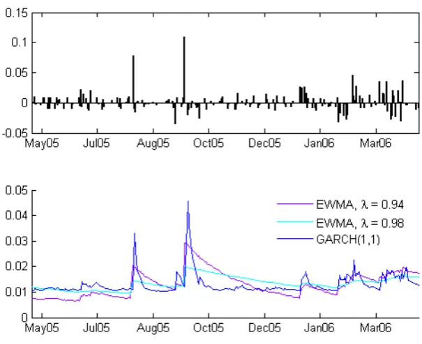
The choice of λ is depending of the behavior desired. Low λ values gives more responsive and rougher behavior in the volatility estimate and highλ values gives less responsive and smoother volatility estimates, see gure 2.3. RiskMetrics2 _{suggests that}_λ_{= 0}_,₉₄ _{should be used for equity and}_λ_{= 0}_.₉₇

for foreign exchange (FX), such as currency trade. The parameter could also be optimized using traditional maximum log-likelihood estimate. With little modication equation (2.9) can be written as:

σ2_t ≈λσ_t2₋₁+ (1−λ)r_t2 (2.10) which is a simple updating formula, where the only variable needed for esti-mating the volatility at time tis the most recent returnrt(the return after

the market closes) and volatilityσt−1 (the estimated volatility from the day

before).

The advantages with the EWMA model is that it only relies on one param-eter, λ, tends to produce much less ghost eects than the historical equal weighted model and a very little data needs to be stored. The main disad-vantages with the EWMA model is that it takesλ to be constant and can therefore be unresponsive to market conditions (Dowd, 2005).

(18)

Figure 2.3: Volatility Estimates for MARL, shows how dierent volatility estimates react to a shock on market

2.4.3 GARCH models

GARCH (generalized autoregressive conditional heteroscedasticity) models proposed by Bollerslev (1986), which was an extension of Engle's (1982) ARCH models, give a solution to this kind of problem. GARCH models can show volatility clustering and leptokurtosis (fatter tails than normal tails) which are two of the most important facts with nancial time series. The GARCH(p, q)model depends onq past volatilities andplast error terms and has the following representation:

(

t=σtzt

σ_t2=ω+Pq

i=1αi2t−i+ Pp

i=1βiσt2−i

(2.11) where the residualst are dened as before as t =rt−r¯. The parameters

must be non-negative and fulll;

q X

i

αi+ p X

i

βi <1

(19)

the residuals. The most common choice is normal distribution, but could also be for example t-distributed (which produces even fatter tails). A max-imum likelihood is ideal for obtaining parameter values (α,β and ω). To obtain the optimal number of parameterskand ptests such as deviance statistics test can be used:

D= 2{`2(M2)−`1(M1)}> cα (2.12)

where `i(Mi) is the maximum log-likelihood parameter for model i. The

maximum log-likelihood of the model with fewer parameters M1 should be

subtracted from the higher number of parametersM2 and compared withcα

which is the(1−α) quantile of theχ2 distribution. Model M1 is rejected if

D > cα in favor ofM2.

GARCH(1,1)

The GARCH(1,1) model is the most popular GARCH model. The reason

is because of its simplicity (depends only on the `last' volatility and return), seems to t most nancial data fairly well (higher values ofk and pusually don't give signicantly better result) and from the principle of parsimony (to choose as simple model as possible to t the data). The model is given as:

σ_t2=ω+α2_t₋₁+βσ2_t₋₁ (2.13) where the parameters must as before be non-negative and fulll α+β <1.

If the governing distribution is assumed to be normal (most common) then the maximum log-likelihood function is obtained as:

` = −n

(20)

The main disadvantages is that the GARCH models are more complex then the other volatility estimates.

Many modication have been developed to the GARCH(1,1) model such

as A-GARCH, E-GARCH, GJR-GARCH, I-GARCH, V-GARCH and many more3_{. Some of those models can explain `leverage eect' which is the}

behav-ior of not responding the same way to negative and positive returns (good and bad news on market), i.e. are asymmetric not symmetric as the GARCH model. Here I will introduce two of them.

GJR-GARCH: Glosten, Jagannathan & Runkle

The GJR-GARCH model (also known as Threshold-GARCH or T-GARCH) was proposed by Glosten, Jagannathan and Runkle (1993) is similar to the GARCH(1,1) model but also exhibits the term St−1 to capture the leverage

eect.

σ2_t =ω+βσ_t2−1+ (α+γSt−1)2t−1 (2.15)

where St−1 = 0 if t−1 ≥ 0 and St−1 = 1 if t−1 < 0, so it doesn't react

the same to positive and negative returns. The GJR-GARCH model has the same parameter restriction as GARCH(1,1), that is α and β must be non-negative (γ can be negative) and fulll:

α+β <1

E-GARCH: Exponential GARCH

The E-GARCH model by Nelson (1991) is a little bit dierent from the GARCH(1,1) and GJR-GARCH, but also captures the leverage eect by letting the volatility estimate depend on the sign of the lagged residual.

ln(σ_t2) =ω+βln(σ_t2₋₁) +α

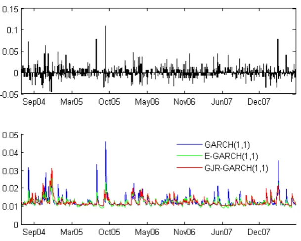
One of the main advantages with the E-GARCH model is that it has no parameter restrictions as the GARCH model. Figure 2.4 shows a compari-son between the GARCH models introduced, GARCH(1,1), E-GARCH and GJR-GARCH. By looking at gure 2.4 the leverage eect can be examined, GARCH(1,1) rises more than the other two when large positive shocks occur and rises less when a short period of negative returns occurs.

3_{see for example Hansen and Lunde (2005) who make a comparison of volatility}

(21)

Figure 2.4: Volatility Estimates for MARL, shows how dierently the GARCH models behave.

2.5 Covariance and correlation

In statistics the covariance gives an estimate of how much two variables change together and is only used when two or more variables are of concern (bivariate or multivariate). For two variablesx and y the covariance can be dened as:

cov(x, y) =E[xy]−E[x]E[y] (2.17)

A strictly related term is the correlation between two variables which gives a measure of how the two variables move together. The correlation is always between−1 and+1 and can be dened as

corr(x, y) = cov(x, y)

σxσy (2.18)

where−1means that instrumentsxandymove totally against each other,0

means that nothing can be said about their movement together and1means

(22)

2.6 ESTIMATING COVARIANCE AND CORRELATION 15

2.6 Estimating covariance and correlation

2.6.1 Historical covariance and correlation

Estimation of covariance and correlation is parallel to estimation of volatility. The historical correlation estimate can be written as:

corr(x, y)t=

and then the covariance could be obtained with:

cov(x, y) =σxσycorr(x, y) (2.20)

2.6.2 EWMA covariance

EWMA covariance can be estimated as:

cov(x, y)t=λcov(x, y)t−1+ (1−λ)xt−1yt−1 (2.21)

and the correlation can be obtained with equation 2.18. As before RiskMet-rics suggests that λ= 0,94 should be used for equity andλ= 0.97 for FX.

To ensure that the matrix is positive denite or semi-positive denite4 _{it is}

important to use the same λvalue for all parameters in the matrix.

2.6.3 GARCH covariance

Since the GARCH based volatility model seem to be powerful tool for the estimation of volatility, it seem to be obvious idea to generate a multivariate version of GARCH estimation. The problem is that multivariate GARCH models are computationally complex and the number of parameters to be estimated grow rapidly as the number of assets in the portfolio grow. Mul-tivariate GARCH models, often called VECH can be written as:

Ht=W+A(t−1T_t−1) +B(Ht−1) (2.22)

where Ht is the vector of volatilities, W is a vector of ω coecients and

A and B are matrix for α and β coecients, respectively. For a portfolio consisting of only two assets the multivariate VECH becomes:

4_{Positive denite or semi-positive denite means in this case that the portfolio volatility}

(23)



Here the total number of parameters to be estimated are 21 and with a 3

asset portfolio the number of parameters needed to be estimated becomes

78. Furthermore this formulation doesn't ensure Ht to be positive denite

(?).

Because of this complexity there has been developed several simplied GARCH based covariance models such as diagonal VECH (DVECH) proposed by Bollerslev, Engle and Woolridge (1988) where the A and B are assumed to be diagonal and the total number of parameters becomes3(k(k+1)/2)where

k is the number of asset in the portfolio, the Constant Conditional Corre-lation model (CCC) proposed by Bollerslev (1990) where total number of parameters becomesk(k+ 5)/2and Dynamic Conditional Correlation model

(DCC) proposed by Engle (2002) where total number of parameters becomes

(k+ 1)(k+ 4)/2. Table 2.1 gives an comparison of parameters needed to be

estimated in multivariate GARCH models.

Number of assets,k VEC DVEC CCC DCC

2 21 9 7 9

3 78 18 12 14

4 210 30 18 20

Table 2.1: Number of parameters to be estimated in multivariate GARCH models

Recent researches such as Sheppard (2003) and Sigurdarson (2007) have shown the advantages with the CCC and DCC model, both because of their `simplicity' (compared to the other) and behavior. I will therefore focus on those two and here I will give a short introduction to them.

Constant conditional correlation, CCC

The model assumes kassets which all are conditionally normal distributed. The covariance matrix,Σt, is dened as:

(24)

2.6 ESTIMATING COVARIANCE AND CORRELATION 17

where Dt is thek×k diagonal volatility matrix, estimated from univariate

GARCH(1,1) process (one at a time as in section 2.4.3)

Dt=

and R is the correlation matrix. The maximum log-likelihood function for the multivariate case when assuming normality can be written as:

` = −1

since the constants don't matter in the maximization. Wherezt∼N(0, R)

whent∼N(0,Σt) are univariate GARCH standardized residuals. The

uni-variate volatility process can be any kind of GARCH process (E-GARCH, GJR-GARCH or some other) and doesn't have to be the same for all as-sets in the portfolio. The correlation is estimated as a constant historical correlation.

R= (ρij) (2.28)

The advantages with the CCC method is that it is much simpler then the full multivariate GARCH model (VECH), a univariate GARCH process can be used for the estimation and the formulation ensures positive deniteness of Ht. The disadvantages is that it assumes the correlation to be constant,

which is unrealistic (?).

Dynamic conditional covariance, DCC

Here the idea is the same in all steps as in CCC except to let the correlation be time varying. A structure for estimating the dynamic correlation was introduced by Engle (2002) as:

Qt= (1−α−β) ¯Q+α(t−1 0

t−1+βQt−1) (2.29)

where_{Q is the}¯ _k_×_k_{unconditional covariance matrix of} _t _and_α _and _β _are

parameters>0, that have to satisfy;α+β < 0. The correlation matrix Rt

(25)

Rt=Q?t−1QtQ?

−1

t (2.30)

where Q?−1

t is obtained as:

Q?−1

t =



  

1 √

q11 0 0

0 ... 0 0 0 √1

qkk



 

 (2.31)

whereqii are thei-th diagonal element of the matrixQt, wherei∈[1, k].

(26)

Chapter 3

Parametric methods

3.1 Univariate parametric methods

In the parametric approach a distribution is tted to the data and the VaR is estimated from the tted distribution. The parametric approach is more appealing mathematically than the non-parametric, since it has a distribu-tion (and density) funcdistribu-tion, which can give a relatively straight forward way of calculating VaR. For example if the normal distribution ts the data well, the VaR atα condence level can be calculated as

VaRα%=µ+σ·zα (3.1)

where zα comes from the standard normal distribution table (' 2.326 for

99%condence level), see gure 3.1.

(27)

If the governing distribution is assumed be student's t-distribution, then the VaR can be calculated as:

VaRα%=µ+ r

υ−2

υ σ·tα (3.2)

with υ degrees of freedom and tα comes from standard t-distribution

ta-ble. If for example the interest would be to nd VaR99% assuming that

t-distribution with 4 degrees of freedom, υ = 4, ts the data well while

µ= 0 and σ= 0.02, then it would be:

VaR99% = r

4−2

4 ·0.02·3.747 = 0.053

while normal distribution would have given VaR99% = 0.047. Here it is

im-portant to understand that volatility tends to be time varying, see section 2.3, therefore the distribution of the residuals is expressed as for example:

rt|Θt∼N(0, σ2t)

where Θt is information set know at time t, for example past returns

{r0, . . . , rt−1} and/or past volatilities {σ0, . . . , σt−1}. Therefore it is said

that the returns rt are conditionally normal distributed, meaning that the

returns at timetare normal distributed conditional on the information set. The choice of distribution can dier a lot. The most common is to assume that normality (that is a normal distribution) is sucient to t the data well, although this has been debated1_{. Other common choice of distributions}

are for example log-normal distribution and extreme value distribution. As stated before, nancial data tend to be clustered, have fat tails and are pos-sibly skewed and thus we would like to t a distribution to the data that can show these characteristics.

3.2 Multivariate parametric methods

Multivariate parametric methods are analogous to the univariate case where assumptions are made about the portfolio rather then a single asset, although making the assumption that each asset in the portfolio is normal is the same as assuming that the portfolio is normal distributed (holds only for normal distribution). With k assets in a portfolio, assuming normal distribution, the VaR can be obtained by:

(28)

3.2 MULTIVARIATE PARAMETRIC METHODS 21

VaRα%=wTr+ √

wT_Σ_w_z_α _(3.3)

see section 2.2 for further details. As beforezαis obtained from the standard

normal distribution. Likewise the for student's t-distributed data portfolio VaRα% can be obtained as:

Correlation can have much eect on VaR estimate which can be shown with a simple example. Suppose we have two equal weighted (w1 = w2 = 0.5)

assets,A1and A2, in a portfolio which both are;A1, A2 ∼N(0,1). The VaR

of each asset is obtained by equation 3.1. The portfolio volatility could be calculated as:

The VaR estimate will be less then the individual VaR estimate for all values of ρ except for ρ = 1 (when short-selling2 is not allowed). So generally it could be stated that:

where VaRi is the Value-at-Risk for asset iin the portfolio. This is one of

the fundamentals with portfolios, called to diversify (see section 2.2). Let's take a simple example. Say that we have two equal weighted assets,A1 and

A2, with are found to have following characteristics; A1, A2 ∼ N(0,0.022)

and the correlation is found to be0.6. We are interested in nding VaR_99%.

Start by nding the portfolio volatility as:

σP = p

0.52_·₀_.₀₂2_{+ 0}_.₅2_·₀_.₀₂2_{+ 2}_·₀_.₆_·₀_.₅_·₀_.₅_·₀_.₀₂_·₀_._{02 = 0}_.₀₁₇₉

and therefore the VaR99% can be obtained as:

VaRα%= 0 + 0.0179·2.326 = 0.0416

2_{In nance short-selling is the act of getting of selling a asset you do not own, in hope}

(29)

while student's t-distribution would have given VaR99%= 0.0474. Both give

lower VaR estimate then in the individual case, found for the univariate sec-tion.

(30)

Chapter 4

Non-parametric methods

4.1 Basic historical simulation

The attempt with the non-parametric models is to let the data (prot/loss or return series) speak for themselves as much as possible, rather than some tted distribution. The main assumption with non-parametric models is that the recent past can be used to model the near future, meaning that some past returns, say two years, are used to model tomorrow's VaR. This way the data (returns) can accommodate any behavior, such as fat tails and skewness, without having to make any distributional assumptions, if the past returns showed that kind of behavior.

The most popular and known non-parametric model is the basic historical simulation (HS). For the basic HS the general idea is to sort the historical returns and estimate the VaR from the sorted historical returns at preferred condence level α. Suppose for example we have 1000 observation of his-torical returns and would want to estimate VaR for tomorrow at a 99%

condence level. We would start by sorting the data, then we would know that 10 returns would lie in `left' of the VaR estimate (1%·1000) and

there-fore a rational estimate of tomorrow's VaR would be the11th one (or some

interpolation between the 10th and the 11th one). Meaning that99% of the

time the loss is not more than the VaR99%.

If for example the15 worst returns the last 4 years have been the following

(LAIS data):

{ -0.0693, -0.0685, -0.0645, -0.0604, -0.0569, -0.0548, -0.0537, -0.0509, -0.0497, -0.0459, -0.0443, -0.0441, -0.0435, -0.0434, -0.0420, ... }

(31)

equals to 1000 days1 _{and 10 observation are allowed to lie `left' of the}

esti-mate)

VaR99% = 0.0443

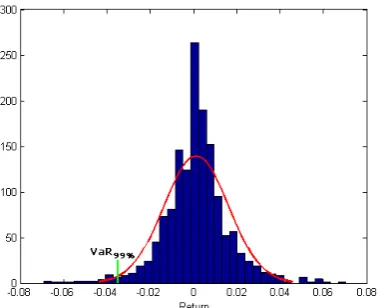
therefore it could be said that we are 99% sure of not getting worse re-turn than 4.43% for tomorrow. Graphically this can be done by plotting a histogram and examine the tail as is shown in gure 4.1

(a) Histogram LAIS data (b) The tail

Figure 4.1: Shows how VaR is obtained graphically with the basic HS

The advantages with the basic HS is that it is really simple. The main dis-advantages is that in the basic HS approach all observations are treated the same, that is all observations have the same weight (called equally-weighted). If all observation are treated the same a shock on the market today could be `averaged' out if the sample size is large enough and not noticed at all except at high condence levels. In other words risk grows without VaR showing it. Another example could be a major nancial crisis in the past. This shock could produce high VaR estimate while it is in the sample space, called `ghost eects', and then produce a jump in the estimate when it falls out of the sample space, see section 2.4.1.

One of the most attractive facts with the non-parametric approaches is that they can be applied as well for a multivariate case as well as univariate case and there is no need for estimating a variance-covariance matrixΣ, which is

often the `dicult' part of a multivariate estimation.

There are several implementations that can be added to the basic HS, such as bootstrapping (re-sampling the data over and over) and combination of non-parametric density function (for being able to treat the data as continuous, not discrete). One of the most popular implementation to the basic HS is to weight the data certain way so that not all observations are treated

(32)

4.2 WEIGHTED HISTORICAL SIMULATION 25

equally. These method's are called `Weighted Historical Simulation' and can be thought as `semi-parametric method' since they combine features of both non-parametric and parametric methods (Dowd, 2005).

4.2 Weighted historical simulation

There are various ways to adjust the data to overcome problems such as `ghost eects'. Here I will introduce few of them.

4.2.1 Age weighted historical simulation (Age-WHS)

Observations are given weight according to their age as them name implies, so that recent (in time) observation will have more weight than older ones. Boudoukh, Richardson and Whitelaw (1998) introduced a formula for calcu-lating observations weight as function of the decay factorλ

w(i) =λi−1 1−λ

1−λn (4.1)

wherew(i)is the weight toidays old observation (i.ew(1)is the weight for

the newest observation) andλis the rate of decay, 0< λ <1. Highλ(close to 1) gives slow rate of decay and low λgives high rate of decay, Boudoukh et al. (1998) recommend using λ= 0.98. As said returns are given weight

according to their age, then the returns are sorted. Their weight's are then summed up, until preferred condence level is achieved and corresponding return will give the VaR estimate.

Boudoukh et al. (1998) age-weighting formula is a nice generalization of basic equal weighted HS (the same as λ→ 1) and gives a more responsive

VaR estimates with a well chosen decay factor,λ. The method is also helpful in reducing ghost eects, since old observation will have had weight close to zero and a large jump is thus less likely to be observed in the sample space.

4.2.2 Volatility weighted historical simulation (VWHS) Proposed by Hull and White (1998) to update the return with volatility changes. As pointed out by them if for example the volatility on market today is1.5%per day on average and two months ago it was 1%on average

then the `old' volatility will give an underestimate for changes in near future and vice versa. They therefore introduced a formula for updating return with volatility as:

r_t?=σT ·

rt

(33)

whereσt is the estimated daily volatility at timet,rtis the historical return

and σT is the most recent estimate of volatility made at the end of date T

Hull and White (1998). More generally, daily returns are standardized with their volatility and then scaled with current volatility. This approach is a straight forward extension of the basic HS where volatility uctuations has been taken into account in estimating VaR. Advanced techniques as EWMA or GARCH process could be used to estimate the volatility process to explain for example volatility clustering. This method has proved a higher estimate of VaR then basic HS (Dowd, 2005).

4.2.3 Filtered historical simulation (FHS)

Approach developed by Barone-Adesi, Bourgoin and Giannopoulos (1998)2

has becoming more and more popular among risk analyzers. First a volatil-ity process is tted to the return (EWMA, GARCH or any other), then the returns (or the residuals, t) are standardized with the volatility estimate

as zt = rt/σt. Here heteroscedasticity should be removed (can be checked

by for example looking at autocorrelation plot, see section 5.2.1). The stan-dardized returnszt are then bootstrapped. Bootstrapping involves drawing

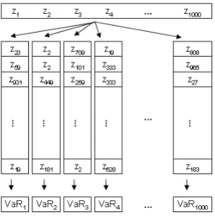
observations randomly from the sample, until the original sample size is reached. This is doneN times (typically 500, 1000 or 5000 times). It should be mentioned that in the bootstrapping procedure the same observation can be drawn more often than once. Finally the new samples are scaled with current volatility σT, and then each sample can give an estimate of

tomor-row's return and the VaR can be obtained at preferred condence level. The procedure is shown graphically on gure 4.2.

Figure 4.2: Bootstrap procedure

(34)

Chapter 5

Analysis

5.1 Methodology

All methods described in chapters 3and 4 are now compared with the goal

of nding the method that gives fewest exceptions and lowest VaR estimate while fullling regulations stipulated by the Basel Committee (2006). By stating as low as possible, the aim is to minimize the regulatory capital, as that is depended on the VaR gure if the internal approach as set forth by the Basel Committee is used. If VaR limit is set very high or overestimated for some reasons, more capital will have to be kept in reserve.

All calculation were done in Matlab. For the multivariate GARCH cal-culations the UCSD Matlab toolbox by Kevin Sheppard was used1_{. As I}

mentioned in section 1.2, VaR has the unit of money, although in the analy-sis I will calculate VaR as a percentage of return for the sake of comparison between dierent instruments. Before going further I will give a short intro-duction to the regulations set by the Basel Committee (see Basel Committee (2006)).

5.1.1 Backtesting

Backtesting is a test performed to check the accuracy of internal VaR model, historically, meaning that over some period (at least 1 year) estimated daily VaR and actual P/L series2 _{are compared and exceptions, when}

−VaRα>Rt, are counted. The internal model is given as:

max{VaRt,

k

60

60 X

i=1

VaRt−i+1} (5.1)

(35)

where VaRtis the 10-day VaR estimate for dayt, andkis known as the

hys-teria factor which is determined by the bank's backtesting result (somewhere between3and4, see section 5.1.2). The reason for using the 10-day VaR, or

10-day holding period, is that it may take that long time to liquidate a posi-tion3_{. For interpolating the 1-day VaR to 10-day VaR the Basel Committee}

allows that the infamous `square-root of time rule' should be used. The rule is given as:

N-day VaR=

√

N×1-day VaR (5.2)

The origin of this rule comes from that if you have 2 independent and iden-tical normal distributed (normal iid) variablesxtandxt+1 with varianceσ2,

the sum of their variance will be:

V ar(xt+xt+1) =V ar(xt) +V ar(xt+1) = 2σ2

Which implies that their volatility is scaled by√2. However this holds only

if all observations are assumed to be normal iid, else it is a approximation (?). Stylized facts such as heteroscedasticity violates the normal iid assumptions and therefore many have debated Basel Committee's recommendation using the square-root of time rule, see for example Daníelsson and Zigrand (2005). The most straight forward way of calculating a 10-day VaR is to use 10 times more data and divide it into 10-day intervals instead of 1-day. This means that for the short period 20 years of data would be needed and for the long period 40 years of data would be needed. The problem is that there are not that many stocks, indices or other nancial time series with such a long history, and those who exist are likely to have changed drastically over last decades (it could thus be debated to use the same model for such a long period). Because of these debates and approximations I will concentrate on calculating 1-day VaR and skip any scaling or interpolations to other time intervals.

5.1.2 Basel zones

The Basel Committee requires that models are at least 99% accurate and

uses a general hypothesis test, in order to balance two types of errors; (I) the possibility that an accurate risk model would be classied as inaccurate on the basis of its backtesting result, and (II) the possibility that an inaccurate model would not be classied that way based on its backtesting result. The Basel Committee categorizes backtesting result into 3 zones to minimize the type I and type II errors. Green zone, indicating that the model is probably good, minimal probabilities of type I error, yellow zone indicating uncertainty

(36)

5.1 METHODOLOGY 29

and possibilities of both types of error and red zone indicating a probably bad model with a minimal chance of type II error. If the model ends in yellow zone it is up to the nancial institution to prove it's goodness (Basel Committee, 2006). Table(1.2)shows the categorization for 1 year of data.

Zone Number of_exceptions _{hysteria factor}Increase in Cumulative_probability

Green Zone

Table 5.1: Backtesting zones in Basel accord based on250 observations

Increase in hysteria factor is what adds to the default,k= 3, in equation 5.1.

The cumulative probability is the binomial probability of getting the num-ber of exceptions or fewer, see equation 5.3. For example the probability of getting 5 exceptions or less is equal to 95,88%, when dealing with 1 year of data and 99%condence.

To interpolate the table to other time intervals the boundaries between green and yellow zone is when the cumulative binomial distribution is equal to/or exceeds 95% and the boundaries between yellow and red zone 99,99%. Lim-its for the short period are therefore, up to8exceptions is green zone, up to 14 is yellow zone and 15 or more will be red zone. For the long period the

limits will be, up to14is green zone, up to22is yellow zone and23or more

will be red zone.

5.1.3 The basic frequency test

(37)

wherenis the number of observations (days),K is the number of exceptions and p is the probability (p = 1−α). In hypothesis testing the idea is to propose a `null-hypothesis'H0 which is assumed to be true (in this case

ex-pected number of exceptions) and a `alternative-hypothesis'H1 which is the

actual outcome from the model. If for example the total number of observa-tionn= 1000, the actual number of exceptionsK= 20, the condence level

α = 0.99 (⇒ p = 0.01) therefore the expected number of exceptions would

be10(1000×0,01) which is less then20, the hypothesis test proposed could

be:

(

H0 :p= 0.01

H1 :p >0.01

More generally, the idea is to check whether the model used for obtainingK exceptions is ok, when the expected number of exceptions isn·p. This is done by putting the values ofn,Kandpare put into equation 5.3 and the results checked. P(K≥20) = 1−P(K ≤19) = 0.0033. Normally5%condence is

used for validating the statistical test (Hull, 2007), therefore the `alternative-hypothesis' would be rejected if P(K =x) is less than the condence level

of the test. In this case P(K ≥ 20) = 0.0033 < 0.05, therefore the

null-hypothesis is rejected, which leads to that the model used for calculating this number of exceptions is rejected. If the number of exceptions had been less than the expected number of exceptions, sayK = 7, the hypothesis had

looked like:

(

H0 :p= 0.01

H1 :p <0.01

and the result had beenP(K≤7) = 0.2189>0.05, and thus the

`alternative-hypothesis' is not rejected and therefore the model used is not rejected (found to be ok).

(38)

5.2 UNIVARIATE CASE 31

5.2 Univariate case

First lets look at univariate analysis. Univariate means that there is only one asset (stock, currency pair, index) underlying. First I will present the results for the parametric approach, then non-parametric and nally compare them together.

5.2.1 Parametric methods

Before modeling the data using parametric approach it is good to try to get as much information from the data as possible, to make as rational decisions as possible. One of those things is to examine the autocorrelation of the data which can give information about repeating patterns in the data. Autocorrelation is given as:

R(k) = E[(Xi−µ)(Xi+k−µ)]

σ2 (5.4)

wherek is the lag between observations. By calculation autocorrelation for the rst two moments, i.e. rt and r2t (or t and 2t), repeating patterns in

the mean and variance can be examined. As has been said before, one of the most stylized facts about nancial time series is that they tend to have autocorrelation in the second moment (the variance, called heteroscedastic-ity). This fact cannot be dismissed, and therefore tting a volatility process that can explain these characteristics should be rational. As was explained in section 2.4.3 a GARCH process is good in simulating heteroscedasticity and could thus be a wise choice.

Here I shown the autocorrelation for the rst two moments for LAIS data long period, see section 1.3 for information on time series.

(a) Autocorrelation int (b) Autocorrelation in2t

(39)

From gure 5.1 there is no indicator of autocorrelation in the rst moment,

the mean (gure (a)) while there is a strong indicator of autocorrelation in the second moment, the variance (gure (b)), almost all lags have autocorre-lation higher then the 95% condence interval. A GARCH process was tted to the data and then the residuals standardized (zt=t/σt). By examining

autocorrelation in the standardized residuals (gure 5.2), it is possible to see whether the tted volatility process did a good job in removing the autocor-relation or not.

(a) Autocorrelation inzt (b) Autocorrelation inzt2

Figure 5.2: Here the autocorrelation is shown for the standardized residuals, LAIS long period.

Figure5.2shows that there is no longer any clear autocorrelation in the

stan-dardized residuals and the next step would be to make some assumptions about the distribution. Similar results were achieved for other assets (see appendix A.1.1).

(40)

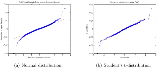
(a) Normal distribution (b) Student's t-distribution

Figure 5.3: Estimating distribution, LAIS long period

From the qq-plots it's clear that Student's t-distribution (with 4 degrees of freedom) ts the LAIS data better then the normal distribution and should therefore be the choice (between those two), although I try both. Figure 5.4 shows the dierence between a normal distribution and Student-t distribu-tion with 4 degrees of freedom.

(a) Normal vs. t distribution (b) Tail behavior

Figure 5.4: The dierence between normal distribution and Student's t-distribution with 4 degrees of freedom

Figure 5.4 shows the characteristic dierence between normal and student's t-distribution (with 4 degrees of freedom).The gure shows that student's t-distribution has fatter tails then the normal distribution, which leads to higher VaR estimate, since the estimate is equal to theα% area under the curve.

Now simulation can take place. Methods described in chapter 3 are

(41)

Figure 5.5: LAIS long period, assuming normal distribution

(42)

Figure 5.7: LAIS shock behavior, assuming normal distribution

(43)

Exceptions were counted and are presented in tables 5.2 to 5.5. In the tables the green color stands for green zone, no color for yellow zone and red color for red zone. Outlined numbers are those where a model has been rejected due to hypothesis testing. The number in brackets is observed exceptions divided by expected number of exceptions.

Method LAIS MARL ERIC NDA ISXI15 OMX EWMA 8(1,6) 9 (1,8) 11 (2,2) 9 (1,8) 11 (2,2) 14 (2,8) GARCH(1,1) 8(1,6) 8(1,6) 13 (2,6) 9 (1,8) 13 (2,6) 16 (3,2) E-GARCH 6(1,2) 8(1,6) 17 (3,4) 8(1,6) 12 (2,4) 14 (2,8) GJR-GARCH 6(1,2) 8(1,6) 12 (2,4) 9 (1,8) 12 (1,4) 14 (2,8)

Table 5.2: Exceptions for the short period, assuming normal distribution

Method LAIS MARL ERIC NDA ISXI15 OMX EWMA 6(1,2) 5(1,0) 9 (1,8) 8(1,6) 6(1,2) 10 (2,0) GARCH(1,1) 4(0,8) 3(0,6) 10 (2,0) 7(1,4) 7(1,4) 9 (1,8) E-GARCH 2(0,4) 2(0,4) 7(1,4) 7(1,4) 9 (1,8) 9 (1,8) GJR-GARCH 2(0,4) 3(0,6) 9 (1,8) 6(1,2) 7(1,4) 10 (2,0)

Table 5.3: Exceptions for the short period, assuming student's t-distribution

Method LAIS MARL ERIC NDA ISXI15 OMX EWMA 16 (1,6) 13(1,3) 23(2,3) 18 (1,8) 20 (2,1) 28(2,8) GARCH(1,1) 15 (1,5) 11(1,1) 20 (2,0) 16 (1,6) 26(2,6) 25(2,5) E-GARCH 16 (1,6) 13(1,3) 24(2,4) 16 (1,6) 25(2,5) 23(2,3) GJR-GARCH 16 (1,6) 13(1,3) 18 (1,8) 15 (1,5) 25(2,5) 23(2,3) Table 5.4: Exceptions for the long period, assuming normal distribution

Method LAIS MARL ERIC NDA ISXI15 OMX EWMA 10(1,0) 8(0,8) 13(1,3) 13(1,3) 13(1,3) 18 (1,8) GARCH(1,1) 7(0,7) 3(0,3) 15 (1,5) 10(1,0) 13(1,3) 16 (1,6) E-GARCH 8(0,8) 2(0,2) 12(1,2) 11(1,1) 17 (1,7) 16 (1,6) GJR-GARCH 8(0,8) 3(0,3) 13(1,3) 10(1,0) 14(1,4) 16 (1,6)

Table 5.5: Exceptions for the long period, assuming student's t-distribution

(44)

LAIS MARL

Method Exceptions VaR σ_VaR max(VaR) Exceptions VaR σ_VaR max(VaR) EWMA 8 0.0324 0.0077 0.0529 9 0.0244 0.0060 0.0558 GARCH(1,1) 8 0.0338 0.0068 0.0526 8 0.0268 0.0065 0.1203 E-GARCH 6 0.0359 0.0087 0.0599 8 0.0268 0.0055 0.0795 GJR-GARCH 6 0.0346 0.0073 0.0532 8 0.0262 0.0063 0.1094

ERIC NDA

Method Exceptions VaR σ_VaR max(VaR) Exceptions VaR σ_VaR max(VaR) EWMA 11 0.0513 0.0248 0.1587 9 0.0367 0.0108 0.0667 GARCH(1,1) 13 - - 0.1242 9 0.0345 0.0094 0.0734 E-GARCH 17 0.0428 0.0098 0.0728 8 0.0346 0.0086 0.0732 GJR-GARCH 12 - - 0.1315 9 0.0344 0.0098 0.0809

ISXI15 OMX

Table 5.6: Detailed information assuming normal distribution, short period

LAIS MARL

Method Exceptions VaR σ_VaR max(VaR) Exceptions VaR σ_VaR max(VaR) EWMA 6 0.0369 0.0088 0.0602 5 0.0278 0.0068 0.0635 GARCH(1,) 4 0.0399 0.0091 0.0657 3 0.0375 0.0132 0.1771 E-GARCH 2 0.0418 0.0105 0.0685 2 0.0662 0.0384 0.2276 GJR-GARCH 2 0.0408 0.0095 0.0681 3 0.0363 0.0118 0.1445

ERIC NDA

Method Exceptions VaR σ_VaR max(VaR) Exceptions VaR σ_VaR max(VaR)

EWMA 9 0.0585 0.0282 0.1807 8 0.0418 0.0123 0.0760 GARCH(1,1) 10 0.0556 0.0208 0.1641 7 0.0395 0.0116 0.0922 E-GARCH 7 0.0551 0.0203 0.1466 7 0.0399 0.0112 0.0923 GJR-GARCH 9 0.0566 0.0263 0.2058 6 0.0395 0.0122 0.1001

ISXI15 OMX

EWMA 6 0.0310 0.0122 0.0634 10 0.0349 0.0094 0.0625 GARCH(1,1) 7 0.0316 0.0146 0.0891 9 0.0330 0.0103 0.0762 E-GARCH 9 0.0316 0.0135 0.0772 9 0.0320 0.0112 0.0689 GJR-GARCH 7 0.0316 0.0144 0.0804 10 0.0324 0.0119 0.0774

(45)

LAIS MARL

Method Exceptions VaR σ_VaR max(VaR) Exceptions VaR σ_VaR max(VaR) EWMA 16 0.0363 0.0121 0.0796 13 0.0277 0.0093 0.0703 GARCH(1,1) 15 0.0370 0.0117 0.0928 11 0.0310 0.0078 0.1203 E-GARCH 16 0.0375 0.0111 0.0775 13 0.0305 0.0074 0.0822 GJR-GARCH 16 - - 0.0799 13 0.0307 0.0080 0.1094

ERIC NDA

Method Exceptions VaR σ_VaR max(VaR) Exceptions VaR σ_VaR max(VaR) EWMA 23 0.0464 0.0207 0.1587 18 0.0317 0.0109 0.0667 GARCH(1,1) 20 - - 0.1242 16 0.0319 0.0087 0.0734 E-GARCH 24 0.0443 0.0136 0.0885 16 0.0315 0.0083 0.0732 GJR-GARCH 18 - - 0.1315 15 0.0318 0.0089 0.0809

ISXI15 OMX

Table 5.8: Detailed information assuming normal distribution, long period

LAIS MARL

EWMA 10 0.0413 0.0138 0.0906 8 0.0316 0.0106 0.0801 GARCH(1,1) 7 0.0449 0.0149 0.1033 3 0.0476 0.0179 0.2257 E-GARCH 8 0.0460 0.0145 0.1012 2 0.1192 0.1659 1.9051 GJR-GARCH 8 0.0457 0.0147 0.1082 3 - - 0.2439

ERIC NDA

EWMA 13 0.0529 0.0236 0.1807 13 0.0362 0.0124 0.0760 GARCH(1,1) 15 0.0526 0.0188 0.1641 10 0.0366 0.0101 0.0922 E-GARCH 12 - - 0.1466 11 0.0366 0.0100 0.0923 GJR-GARCH 13 - - 0.2058 10 0.0366 0.0107 0.1001

ISXI15 OMX

EWMA 13 0.0293 0.0116 0.0634 18 0.0289 0.0110 0.0633 GARCH(1,1) 13 0.0300 0.0132 0.0891 16 0.0288 0.0098 0.0762 E-GARCH 17 0.0300 0.0125 0.0772 16 0.0283 0.0099 0.0689 GJR-GARCH 14 - - 0.0823 16 0.0288 0.0108 0.0774

(46)

The models give fairly similar results. EWMA, E-GARCH and GJR-GARCH give 11 green zones out of 24 and GARCH(1,1) 10 out of 24. When means, standard deviations and minimum values are examined, it comes clear that EWMA usually has the lowest mean and minimum values while GARCH based methods have the lowest standard deviations. This supports descrip-tions given in section 2.3, i.e. GARCH models are quicker to simulate market condition and spike higher, while EWMA is slower to follow market uctu-ations (see gures 5.7 and 5.8). The GARCH models are more sensitive than the EWMA model, especially GJR-GARCH, and fails on getting re-sults when high jumps occur in time series (MARL and ERIC). Finally I compare the parametric results with the extra long currency pair time series (10 years). Exceptions, means, standard deviation and minimum values are given in table 5.10.

Normal distribution Student's t-distribution Method Exceptions VaR σ_VaR min(VaR) Exceptions VaR σ_VaR min(VaR)

EWMA 44 0.0179 0.0076 0.0591 22 0.0204 0.0086 0.0673 GARCH(1,1) 31 0.0179 0.0073 0.1036 14 0.0206 0.0081 0.0855 E-GARCH 42 0.0172 0.0081 0.1537 18 0.0199 0.0079 0.0853 GJR-GARCH 32 - - 0.1389 18 - - 0.1046

Table 5.10: Detailed information, currency pair

For the currency pair GARCH and GJR-GARCH has green zones for both distribution, while EWMA and E-GARCH has only green zone when t-distribution is assumed to be the governing t-distribution of the residuals. Means, standard deviation and maximum values are pretty similar between the methods. Here it is worth mention that although a frequency test would suggest to reject models who have 17 or fewer exceptions they will not be rejected because of central limit theorem4_.

Altogether none of the method is showing any superior characteristics. E-GARCH and GJR-E-GARCH do not improve the regular E-GARCH signicantly and seem to be more sensitive than the regular one. E-GARCH has though the tendency to lower the VaR, which is appealing. Since GARCH is known to be better in explaining fat tails and heteroscedasticity it is recommended as a rst choice, but since EWMA isn't giving any fewer green zones it is recommended as second choice. It could thus be wise to model both for the sake of comparison and to minimize model and implementation risk.

4_{Central limit theorem indicates that if you for example toss a fair dice 10 times the}

(47)

5.2.2 Non-parametric methods

For the non-parametric case any distributional assumption aren't necessary and therefore a pre analysis on the data isn't needed. Calculation for all the non-parametric method's described in the chapter 4 were done for the

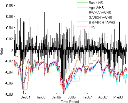
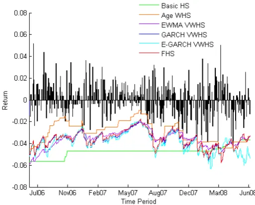
data. For the FHS simulation a GARCH(1,1) process was used to standard-ize returns and 1000 bootstraps were used. The mean of those 1000 were taken as the nal solution. Solutions for all calculation are in tables. Here I present only LAIS gures (see gures 5.9 and 5.10) , the rest is in appendix.

(48)

Figure 5.10: LAIS short period

Exceptions where counted and are displayed in tables 5.11 and 5.12. Over-lined numbers indicates that the model is rejected due to hypothesis testing (too few exceptions). Color indicates which zone the model ends in (green means green zone, no color means yellow zone and red means red zone).

Method LAIS MARL ERIC NDA ISXI15 OMX Basic HS 1(0.2) 4(0.8) 8(1.6) 6(1.2) 7(1.4) 7(1.4) Age WHS 13 (2.6) 13 (2.6) 12 (2.4) 12 (2.4) 15(3.0) 14 (2.8) EWMA VWHS 11 (2.2) 13 (2.6) 11 (2.2) 7(1.4) 11 (2.2) 8(1.6) GARCH(1,1) VWHS 7(1.4) 6(1.2) 10 (2.0) 8(1.6) 8(1.6) 8(1.6) E-GARCH VWHS 5(1.0) 8(1.6) 11 (2.2) 6(1.2) 9 (1.8) 10 (2.0) FHS 7(1.4) 9 (1.8) 9 (1.8) 8(1.6) 8(1.6) 7(1.4)

Table 5.11: Exceptions for the short period

Method LAIS MARL ERIC NDA ISXI15 OMX Basic HS 15 (1,5) 8(0,8) 13(1,3) 13(1,3) 19 (1,9) 14(1,4) Age WHS 27(2,7) 30(3,0) 26(2,6) 27(2,7) 31(3,1) 31(3,1) EWMA VWHS 22 (2,2) 21 (2,1) 23(2,3) 18 (1,8) 27(2,7) 22 (2,2) GARCH(1,1) VWHS 17 (1,7) 11(1,1) 17 (1,7) 13(1,3) 24(2,4) 15 (1,5) E-GARCH VWHS 16 (1,6) 13(1,3) 17 (1,7) 11(1,1) 23(2,3) 17 (1,7) FHS 17 (1,7) 11(1,1) 15 (1,5) 13(1,3) 22 (2,2) 15 (1,5)

Table 5.12: Exceptions for the long period

(49)

LAIS MARL

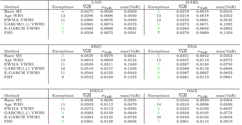
Method Exceptions VaR σ_VaR max(VaR) Exceptions VaR σ_VaR max(VaR) Basic HS 1 0.0475 0.0048 0.0563 4 0.0278 0.0018 0.0316 Age WHS 13 0.0296 0.0096 0.0450 13 0.0218 0.0078 0.0352 EWMA VWHS 11 0.0305 0.0076 0.0490 13 0.0223 0.0061 0.0545 GARCH(1,1) VWHS 7 0.0365 0.0074 0.0578 6 0.0273 0.0071 0.1285 E-GARCH VWHS 5 0.0383 0.0090 0.0632 8 0.0264 0.0056 0.0862 FHS 7 0.0358 0.0075 0.0581 7 0.0270 0.0069 0.1259

ERIC NDA

ISXI15 OMX

Table 5.13: Detailed information, short period

LAIS MARL

ERIC NDA

ISXI15 OMX

Table 5.14: Detailed information, long period

(50)

GARCH VWHS has the highest maximum values in most of the times, al-though the dierence between the VWHS isn't that much most of the time. The Age WHS gives the poorest result, a red zone for all the cases in the long period.

Results for the extra long currency pair modeling are given in table 5.15. USDISK

Method Exceptions VaR σ_VaR max(VaR) Basic HS 44 0.0177 0.0036 0.0277 Age WHS 57 0.0172 0.0077 0.0523 EWMA VWHS 38 0.0178 0.0057 0.0408 GARCH(1,1) VWHS 29 0.0188 0.0067 0.0992 E-GARCH VWHS 37 0.0180 0.0077 0.1514 FHS 32 0.0186 0.0067 0.0976

Table 5.15: Detailed information, currency pair

Result for the currency pair supports the result from the stock and index analysis. GARCH VWHS and FHS have green zones, while AGE WHS gives red zone and the rest yellow zone.

(51)

5.3 Multivariate case

As for the univariate case I rst present the results for the parametric ap-proach and then the non-parametric apap-proach. For the parametric apap-proach methods described in section 3.2 are calculated with covariance estimated as described in section 2.6.1.

5.3.1 Parametric methods

As in the univariate case plotting qq-plots can be helpful to see what distri-bution ts the data well. As before I check how the residuals t to normal distribution and students t-distribution.

(a) Normal distribution (b) Student's t-distribution

Figure 5.11: Estimating distribution for Portfolio 1

As for the univariate case, student's t-distribution (with 4 degrees of freedom) ts the residuals better then the normal distribution, although as before I will try both. Portfolios described in section1.3 are analyzed and VaR

esti-mate is obtained both with multivariate EWMA and multivariate GARCH models. For the multivariate GARCH models, CCC and DCC, the univari-ate volatility estimunivari-ates in matrix Dt (see equation 2.25) are all obtained by

(52)

5.3 MULTIVARIATE CASE 45

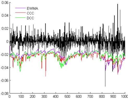
Figure 5.12: Multivariate case, assuming normal distribution

Figure 5.13: Multivariate case, assuming Student's t-distribution

(53)

Figure 5.14: Multivariate case, assuming normal distribution

Figure 5.15: Multivariate case, assuming Student's t-distribution

Finally exceptions are counted and presented in tables 5.14 and 5.15. EWMA†

and GARCH(1,1)† _{stands for EWMA and GARCH(1,1) without taking}

(54)

5.3 MULTIVARIATE CASE 47

Method Portfolio 1 Portfolio 2 EWMA† ₁_(0.1) ₀_(0.0)

GARCH(1,1)† ₂_(0.2) ₄_(0.4)

EWMA 22 (2.2) 14(1.4) CCC 18 (1.8) 15 (1.5) DCC 17 (1.7) 16 (1.6)

Table 5.16: Exceptions for the multivariate case, assuming normality

Method Portfolio 1 Portfolio 2 EWMA† ₀_(0.0) ₀_(0.0)

GARCH(1,1)† ₁_(0.1) ₀_(0.0)

EWMA 13(1.3) 12(1.2) CCC 13(1.3) 12(1.2) DCC 19 (1.9) 13(1.3)

Table 5.17: Exceptions for the multivariate case, assuming t-distribution

As can be seen from the gures 5.14 and 5.15 and tables 5.16 and 5.17 not taking covariances into account raises the VaR estimate a lot, as was ex-pected (see section 2.5), and with hypothesis testing all of the cases when correlation are not taken into account are rejected due to too few excep-tions. Further analysis of means, standard deviations and maximum values are presented in tables 5.18 and 5.19.

Portfolio 1 Portfolio 2

EWMA† ₁ _0.0353 _0.0087 _0.0615 ₀ _0.0341 _0.0085 _0.0632

GARCH(1,1)† ₂ _0.0373 _0.0060 _0.0668 ₄ _0.0355 _0.0066 _0.0673

EWMA 22 0.0223 0.0073 0.0492 14 0.0235 0.0070 0.0461 CCC 18 0.0240 0.0047 0.0538 15 0.0249 0.0067 0.0535 DCC 17 0.0223 0.0059 0.0464 16 0.0247 0.0067 0.0530

Table 5.18: Detailed information assuming normal distribution

Portfolio 1 Portfolio 2

Method Exceptions VaR σ_VaR max(VaR) Exceptions VaR σ_VaR max(VaR) EWMA† ₀ _0.0403 _0.0098 _0.0702 ₀ _0.0389 _0.0096 _0.0720

GARCH(1,1)† ₁ _0.0424 _0.0068 _0.0761 ₀ _0.0404 _0.0075 _0.0766

EWMA 13 0.0255 0.0082 0.0560 12 0.0267 0.0080 0.0526 CCC 13 0.0240 0.0047 0.0538 12 0.0263 0.0064 0.0658 DCC 19 0.0219 0.0044 0.0532 13 0.0258 0.0064 0.0657

Table 5.19: Detailed information assuming Student's t-distribution