Semi Supervised WSD in Selectional Preferences with Semantic Redundancy

(1)

Semi-Supervised WSD in Selectional Preferences

with Semantic Redundancy

Xuri TANG

1,5

, Xiaohe CHEN

1

, Weiguang QU

2,3

and Shiwen YU

4

1. School of Chinese Language and Literature, Nanjing Normal University

{xrtang,chenxiaohe5209}@126.com

2. Jiangsu Research Center of Information Security & Privacy Technology

3. School of Computer Science, Nanjing Normal University

[email protected]

4. Institute of Computational Linguistics , Peking University

[email protected]

5. College of Foreign Studies, Wuhan Textile University

Abstract

This paper proposes a semi-supervised approach for WSD in Word-Class based selectional preferences. The approach exploits syntagmatic and paradigmatic semantic redundancy in the semantic system and uses association computation and minimum description length for the task of WSD. Experiments on Predicate-Object collocations and Subject-Predicate collocations with polysemous predicates in Chinese show that the proposed approach achieves a precision which is 8% higher than the semantic-association based baseline. The semi-supervised nature of the approach makes it promising for constructing large scale selectional preference knowledge base.

1

Introduction

This paper addresses word sense disambiguation (WSD) which is required in the construction of selectional preference (SP) knowledge database. In previous literature of SP, four different types of formalization models are explicitly or implicitly employed. Two types are distinguished in Li and Abe(1998):

Word Model:

P

(

n

|

v

,

r

)

=

σ

(1) Class Model:

P

(

C

|

v

,

r

)

=

σ

(2)

where v stands for verb, n for noun, C for the semantic class of n, r for the grammatical relation between v and n, and P for the preference strength. Most of the researches(Resnik 1996; Li and Abe 1998; Ciaramita and Johnson 2000; Brockmann and Lapata 2003; Light and Greiff 2002) uses the class model, and a few(Erk 2007) uses the word model. The other two types of model are given as below:

Class-Only Model: _P(_C_n|_C_v,_r)=σ (3) Word-Class Model: P(n,Cn|v,Cv,r)₌σ (4) where , are semantic classes for the noun and verb respectively. Class-Only model considers solely the semantic classes, while Word-Class model considers both words and semantic classes. Agirre and Martinez(2001) and Zheng et al(2007) adopted the Class-only Model in research, while in McCarthy and Carroll(2003) and Merlo and Stevenson(2001) the Word-Class Model is employed.

n

C

v

Among the four models, the Word-Class Model is the type which possesses the most granulated knowledge and is the most potential in applications. McCarthy and Carroll(2003) reports that the Word-Class Model performs well in unsupervised WSD. In other NLP tasks such as metaphor recognition, this model may be indispensable. For instance, to distinguish the predicate verb “⍂ࡼ(float)” in Ex(1a) as

Ex. 1

a. ᷥ ৊ ⍂ ࡼleaf floats b.

Ӌ Ḑ ⍂ ࡼ

(2)

literal and Ex(1b) as metaphorical requires different interpretations of the verb.

The present research is concerned with WSD as in the Word-Class model. Particularly, it aims at disambiguating predicates in subject-predicate (Subj-Pred) and subject-predicate-object (Pred-Obj) constructions. The motivations behind the research are two folds. Firstly, semi-supervised and unsupervised WSD in SP are not fully explored. Merlo and Stevenson(Merlo and Stevenson 2001) employs supervised learning from large annotated corpus, which is difficult to obtain. One known unsupervised learning approach for WSD in SP is McCarthy and Carroll(2003) which addresses the issue via conditional probability. The other motivation derives from the fact few research is done on selectional preferences in languages other than English, as is stated in Brockmann and Lapata(2003). For instance, studies on construction of SP knowledge database in Chinese can only be found in Wu et al(2005), Zhen et al(2007), Jia and Yu(2008) and some others.

The basic idea of the approach proposed for WSD in the paper is that the most acceptable interpretation of senses for a given construction is the pair of senses which encodes the most redundant information in the semantic system of the language. Two principles, namely Syntagmatic Redundancy Principle and Paradigmatic Redundancy Principle, are proposed in the paper to capture the intuition. Two corresponding devices are employed to model the two principles: Association for Syntagmatic Redundancy Principle and Minimum Description Length for Paradigmatic Redundancy Principle. Two experiments are conducted in the paper. The first is based on semantic association, achieving a 61.98% precision for predicates in Subj-Preds and 62.54% in Pred-Objs. This experiment is used as baseline as the approach is also used in McCarthy and Carroll(2003) for verb and adjective disambiguation. In the second experiment, both semantic association and MDL are employed, the precision of WSD amounts to 69.88% and 69.09% for predicates in Subj-Preds and Pred-Objs respectively, indicating that a combination of the two devices are fairly effective in disambiguating word senses for SP.

The rest of the paper is organized as below. The second part gives further illustration of the rationale for the approach. The third part describes the procedure and the fourth part discusses the experiment result. The thesis concludes with some speculations in further researches.

2

Rationale

2.1 Task Formalization

Consider a Subj-Pred or Pred-Obj collocation C=< , > , where is

the word of predicate and is the word of

argument. has M senses, denoted by set

. has N senses, denoted by .

The possible interpretation of C has M*N

possibilities, denoted by ={ | =< , >},

where is called a sense collocation. The

task of WSD is to search for a particular sense collocation in and assign it to C as its interpretation. At the initial stage, each sense collocation in is considered to have an even number of frequency, namely

. Accordingly, for each

, , For each

2.2 Syntagmatic Redundancy Principle

Syntagmatic Redundancy Principle (SRP) can be stated as following: among all possible sense collocations for a word collocation, the most appropriate is the one in which senses exhibit the most redundant information between each other.

(3)

and emphasizes that the meanings of collocationally restricted lexemes such as “bark” and “fell” can only be explained by taking into account the collocates they occur with. This notion is also employed in Yarowsky(1995) for WSD, in which the key is the “one-sense-per-collocation” statement. McCarthy and Carroll(2003) also uses this type of redundancy for disambiguation in SP.

SRP can be explained as a statistic correlation between and . The more

co-relevant these two senses are, the more likely the pair is to be accepted as the appropriate interpretation. This can be described as below:

pred

where is the function for

sense association. Four methods can be considered for association computation: conditional probability (Formula 6 and 7), Lift(Han and Kamber 2006:261) (Formula 8), All-Confidence(Han and Kamber 2006:263) (Formula 9) and cosine (Formula 10). Note that two versions of conditional probability are considered, as are denoted in Formula 6 and 7. The first version, Cond-Prob 1, takes argument sense as condition, while the second version Cond-Prob 2 takes predicate sense as condition.

2.3 Paradigmatic Redundancy Principle

Paradigmatic Redundancy Principle (PRP) can be stated as following: among all possible sense collocations for a word collocation, the most appropriate is the one which is also implicitly or explicitly expressed by other synonymous, metonymic or metaphorical word collocations.

Ex(2) illustrates the explicit redundancy in synonymous and metaphorical ways, in which the sense collocation “[Price| Ӌ Ḑ ] [QuantityChange|䞣ব]” is expressed by five word collocations, each with a different predicate : ব ࣪(change), ⍂ ࡼ(float), 䇗 ᭈ (adjust),䍋ӣ(go up and down), বࡼ(alter).

Ex 2.

a.ӋḐব࣪_{price changes}

b.

Ӌ Ḑ ⍂ ࡼ_{price floats}

c.

Ӌ Ḑ 䇗 ᭈ_{price adjusts}

d.

Ӌ_{SULFHJRHVXSDQGGRZQ}Ḑ 䍋㨑

e.

Ӌ Ḑ ব ࡼprice alters

Ex(3) reveals the implicit redundancy in metonymic way, in which the meaning “Ҏ (human) ᅝ ᖗ (is eased)” is implicitly expressed in all the six collocations, established by semantic relatedness among the arguments “偀 ᢝ ໮ 㒇(Maradona)”, “ᄺ ⫳

labour is eased

e.

㸠䔺 ᅝᖗ њ_{driving is eased}

f.

⫳⌏ ᅝᖗ њ_{Life is eased}

To apply PRP, WSD in SP is casted as an issue of model selection. Given a set of word collocations , the process of WSD is to assign to each word collocation one sense collocation from a number of possibilities. Those assigned sense collocations form a set, or a model for Θ. The goal of WSD in SP is to select from all those models the one which best interprets Θ. For this purpose, Miminum Description Length(Barron et al. 1998; Michell 2003; MacKay 2003) can be used. MDL selects models by relying on induction bias based on Occam’s Razor, which stipulates that the simplest solution is usually the correct one. One way to interpret MDL in Bays’ analysis is as below(Michell 2003:124):

Θ

is the data description length when model is used for description. The model with minimum length is the best model.

(4)

For model description length, we have adopted the method used in (Li and Abe 1998) which considers only the size of the model:

)

where size(m) is the number of sense collocation contained in model _m, and N is the number of word collocation in consideration. In this study, the set of word collocation with the same predicate word, denoted by Θ, is used as the unit for model description length calculation instead of the whole corpus, so as to reduce computation complexity. Accordingly, each word collocation in Θ can be assigned one and only one sense collocation in the model m, out of all the potential sense collocations as is explained in section 2.1.

Data description length is calculated on model and , as is denoted in formulas

based on the probability of sense collocation , which in turn is calculated on a

modified frequency of the collocation

>

The frequency is modified by counting the explicit occurrence of the sense collocation itself and the implicit occurrence expressed by other sense collocations in Θ . This idea is equivalent to enlarge the corpus by 1 fold, thus the overall collocation number is the two times of the original number.

The modified frequency is a sum of two parts, denoted in formula (14). The first part is

, the frequency of . The second part is

the weighted frequency of . The weight is

determined by the relatedness of the sense collocation and all the other sense

collocation in the model m. According to this formula, if the sense collocation is found to be more similar to other sense collocations, it should obtain a higher modified frequency,

and thus more likely to be the correct one for the word collocation.

)

The way to calculate the weight is given in formula (15). If two sense collocations have identical predicate sense, namely ,

then the weight between the two sense collocations is measured by _rel , the

semantic relatedness between the argument sense and . Otherwise, 0 is returned.

There are different ways to measure sense relatedness. The present study has used semantic similarity based on HowNet(Liu and

i 2002) to calculate the semantic relatedness.

k

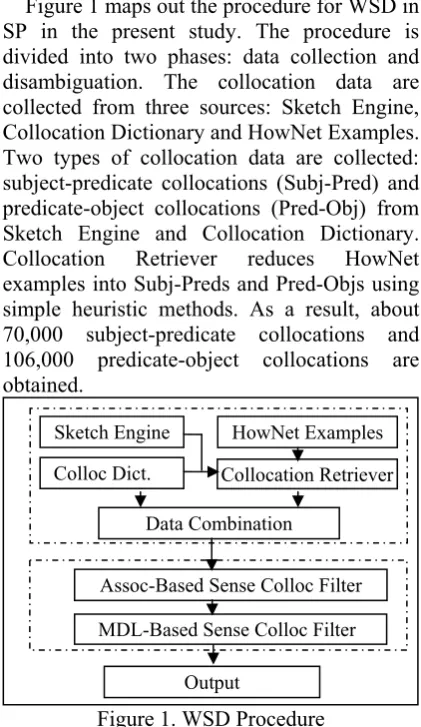
Figure 1 maps out the procedure for WSD in SP in the present study. The procedure is divided into two phases: data collection and disambiguation. The collocation data are collected from three sources: Sketch Engine, Collocation Dictionary and HowNet Examples. Two types of collocation data are collected: subject-predicate collocations (Subj-Pred) and predicate-object collocations (Pred-Obj) from Sketch Engine and Collocation Dictionary. Collocation Retriever reduces HowNet examples into Subj-Preds and Pred-Objs using simple heuristic methods. As a result, about 70,000 subject-predicate collocations and 106,000 predicate-object collocations are obtained.

Figure 1. WSD Procedure

In disambiguation phase, two devices are employed to filter out unlikely sense collocations: Association-Based Sense Collocation Filter, following SRP, and MDL-Based Sense Collocation Filter, following PRP.

Colloc Dict.

HowNet Examples

MDL-Based Sense Colloc Filter Assoc-Based Sense Colloc Filter

Collocation Retriever

Data Combination Sketch Engine

(5)

In this phase, Subj-Preds and Pred-Objs are processed independently but following the same route.

Each phase alone can perform WSD independently. Accordingly, two experiments are conducted to evaluate the method proposed in this paper. The first experiment uses association-based filter for word sense disambiguation, which is also used as the baseline. The approach is also used in (McCarthy and Carroll 2003) to disambiguate verbs and adjectives in collocations. To be particular, the method used by McCarthy and Carroll(2003) is formula (6). The second experiment is based on the result of the first one so as to observe the improvement obtained by MDL-Based approach. In the second experiment, unsupervised and semi-supervised WSD are also investigated by including some annotated collocations in the evaluation data.

Two corpora are constructed for evaluation. One corpus is a set of 1034 subject-predicate constructions. The other is a set of 1841 predicate-object constructions. Both are manually annotated by the authors with sense definitions defined in HowNet(Dong 2006). All together there are 52 highly ambiguous predicates involved in the study.

4

Experiments and Discussion

4.1 Collocation Retriever

The major task in data collocation is in Collocation Retriever, which retrieves collocations from HowNet examples. Ex(4) gives a partial entry structure in HowNet,

Ex 4.

W_C=⍂ࡼ

E_C=Ҏᖗ~ˈᓔྟ~ˈᎹ԰ᣛᷛϡذ

ഄ~

DEF=[change|ব]

in which W_C stands for Chinese Word, DEF for definition, E_C for Examples of Chinese, and the wave “~” for the word in question. From E_C, possible Subj-Preds such as “Ҏᖗ (public opinion) ⍂ࡼ(floats)”, “ᣛᷛ(index) ⍂ࡼ(floats)” can be retrieved, in which the sense of “⍂ࡼ(float)” is annotated with DEF. But there are also noises. A simple heuristic method is applied to automatically filter out unwanted collocations. The heuristic method

checks whether the collocation retrieved from HowNet share possible sense collocations with collocations in Collocation Dictionary. If yes, it is accepted as a collocation of the type, otherwise, it is rejected. Procedures are given below:

(a) Use Subj-Pred collocations and Pred-Obj collocations in Collocation Dictionary to build sense collocation set

ed Subj−Pr

Γ and _Γ_Pr_ed₋_Obj; (b) For each example sentence in E_C, segment it using ICTCLAS1 to obtain an array of words. Words before “~” forms potential Subj-Pred collocations and Words

after form potential Pred-Obj collocations .

ed Subj−Pr

Α

Obj ed

BPr −

(c) For each or ,

construct possible sense collocation set

ed Subj

a∈Α −Pr b∈BSubj−Pred

a

Γ

or

b

Γ , if _Γ _∩_Γ ₋ _≠_φ

ed Subj

a Pr or Γb ∩ΓPred−Obj ≠φ, add it as a Subj-Pred collocation or Pred-Obj collocation.

Evaluation on partial retrieved collocations shows that about 70% of obtained collocations are valid collocations, while about 30% are errors. Thus manual edition has been applied to rid those invalid collocations.

4.2 Association-Based Filter

Association-Based Sense Collocation Filter filters out those sense collocations that are very unlikely to be the right interpretation for a word collocation. Table 1 gives association computation result for the six senses related to the predicate “ ㉫ (rough)” in Subj-Pred collocation “ᗻ Ḑ(personality) ㉫(rough)”. The 2nd , 3rd, 4th, and 6th are very unlikely interpretations and should be filtered, while the 5th seems to be the most appropriate.

Following the procedure in Figure 1, to filter out those unlikely sense collocations, average

1

A Chinese segmentation system, please refer to

(6)

association value is used as the filter and those below the average are dropped and those above are chosen for MDL-Based Filter. In Table 1, the average is 0.0017, and the 1rd and 5th are chosen.

However, in order to obtain a baseline and to decide which association computation model to use, we have followed the definition in Formula 5 and perform WSD test by choosing the sense collocation with highest association as the correct sense tags. for used this step solely for WSD, as is defined in Formula 4. Table 2 gives the experiment results for Subj-Pred and Pred-Obj collocations with all the association computation models denoted in Formula 6-10.

Table 2. WSD Result by Association Subj-Pred(%) Pred-Obj(%) Cond-Prob 1 61.98 62.54 Cond-Prob 2 55.15 42.4 Lift 63.09 40.84 All_Conf 56.16 48.54 Cosine 58.83 55.72

One interesting phenomenon about all the five models is null-invariance. In selecting models for association computation, null-invariance is an important feature to be considered(Han and Kamber 2006). A model with null-invariance is not influenced by additional irrelevant data and thus is more stable. In the experiment, the model Lift is the only one not featured with null-invariance. The experiments show that Lift is not stable in different collocation types, achieving high precision in Subj-Pred but low precision in Pred_Obj.

A second interesting phenomenon is collocation directionality exposed by the experiments, which can be observed in the two models of conditional probability: Cond-Prob 1, with argument as condition, and Cond-Prob 2, with predicate as condition. Directionality in collocation has been noticed earlier in some researches, for example Qu(2008). Our experiment shows that when using Cond-Prob 1, we are able to get a precision of 61.98% and 62.54% for Subj-Pred and Pred-Obj respectively, while Cond-Prob 2 gets a much lower precision. This fact can be interpreted that arguments tend to have a stronger selectional preference strength, and the possible selection range is comparatively narrower, while predicates have weaker

selectional preference strength and a wider selectional range.

4.3 MDL-Based Filter

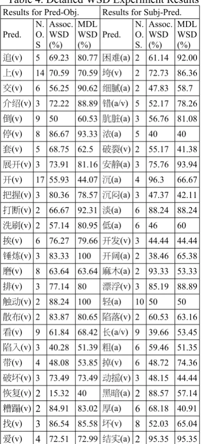
MDL-Based Filter takes as input result from Association-Based Filter using Cond-Prob 1 for association computation and average association as filter. Table 3 and 4 give the final experiment outcome for Pred-Obj and Subj-Pred constructions and individual predicates.

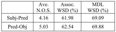
It can be seen in Table 3 that MDL-Based Filter Several inferences can be made from the experiments. Firstly, comparison between Association-Based WSD (Table 2) and MDL WSD (Table 3) shows that MDL can improve overall performance up to 8%. As is mentioned earlier, Association-Based WSD is used as baseline in the present study. Given the fact that the average number of senses for word in question is fairly high, the improvement is considered as significant.

Table 3. General WSD Results2 Ave.

N.O.S.

Assoc. WSD (%)

MDL WSD (%) Subj-Pred 4.16 61.98 69.09

Pred-Obj 5.03 62.54 69.88 Analysis on the individual predicates in Table 4 gives a clearer picture of WDL-based WSD. Firstly, it can be seen that MDL is especially effective when the demarcation of word senses is clear-cut. Predicate words such as “ᅝ 䴭(quiet)”, “㚂㛣(dirty)”, “ೄ 䲒 (difficult)” in Subj-Preds and “䫸 ⚐(beat)”, “㾺ࡼ(touch)” and “ᠧᮁ(break)” in Pred-Objs are successfully disambiguated in Table 4. These words generally have 2 or 3 senses, and the senses generally differ in terms of abstractness and concreteness, as is indicated in table 5. This is due to the fact that the arguments in these collocations are clearly delimitated in HowNet and this delimitation is well captured by the modified frequency calculation defined in formula (14). Via the formula, the concrete sense collocations can

2

(7)

Table 4. Detailed WSD Experiment Results Results for Pred-Obj. Results for Subj-Pred.

Pred. N. O. S

Assoc. WSD (%)

MDL WSD (%)

Pred. N. O. S.

Assoc. WSD (%)

MDL WSD (%) ಳ(v) 5 69.23 80.77 ܺ呕(a) 2 61.14 92.00 Ղ(v) 14 70.59 70.59 ৅(v) 2 72.73 86.36 ٌ(v) 6 56.25 90.62 伟俩(a) 2 47.83 58.7 տ伦(v) 3 72.22 88.89 原(a/v) 5 52.17 78.26 ଙ(v) 9 50 60.53 ᴂ俓(a) 3 56.76 81.08 ೖ(v) 8 86.67 93.33 䳚(a) 5 40 40 ୚(v) 5 68.75 62.5 ధါ(v) 2 55.17 41.38 ୶䬞(v) 3 73.91 81.16 ڜ䈌(a) 3 75.76 93.94 䬞(v) 17 55.93 44.07 ި(a) 4 96.3 66.67 ނ༽(v) 3 80.36 78.57 ި吚(a) 3 47.37 42.11 ؚ㵱(v) 2 66.67 92.31 ෉(a) 6 88.24 88.24 ੑࠧ(v) 2 57.14 80.95 ܅(a) 6 46 60 ஬(v) 6 76.27 79.66 䬞䦡(v) 3 44.44 44.44 厪䴨(v) 3 83.33 100 䬞吷(a) 2 38.46 65.38 ᗣ(v) 8 63.64 63.64 ຾ֵ(a) 2 93.33 53.33 ඈ(v) 3 77.14 80 ዦ௬(v) 3 85.19 88.89 ⡣㣅(v) 2 88.24 100 剥(a) 10 50 50 ཋؒ(v) 2 83.87 80.65 ະᆵ(v) 2 60.53 63.16 ઎(v) 9 61.84 68.42 叿(a/v) 9 39.66 53.45 ະԵ(v) 3 40.28 51.39 ษ(a) 6 59.46 51.35 䬈(v) 4 48.08 53.85 ൾ(v) 6 48.72 74.36 ధ݅(v) 3 73.49 73.49 㣅㿼(v) 3 48.15 44.44 ਀ᵵ(v) 2 15.32 40 ႕ᄆ(a) 2 88.57 57.14 ᜊᝡ(v) 2 84.91 83.02 দ(a) 6 68.18 40.91 ބ(v) 3 86.54 85.58 ݅(v) 8 52.03 65.04 䵋(v) 4 72.51 72.99 伬㨕(a) 2 95.35 95.35

Table 5. Word Sense Distinction

Pred Concrete Sense Abstract Sense(s) ڜ䈌 [quiet|䈌] [calm|反䈌],

[peaceful|᩶] ᴂ俓 [dirty|囀] [despicable|࠲٭],

[immoral|լሐᐚ] ܺ呕 [difficult|呕] [poor|乳]

increase the modified frequency of concrete sense collocations, and the abstract sense collocation can increase the modified frequency of abstract sense collocations, thus

leading to the clear demarcation of abstract senses and concrete senses.

The role of semantic relevance can also be clearly noticed in the predicates which have a decreased precision in MDL in Table 4. Via Paradigmatic Redundancy Principle, the information encoded in one collocation are diffused to other collocations. Consequently, errors can be diffused. This explains why the precisions of some predicates such as “≝ (sink)”, “咏᳼(dumb)”, “咥ᱫ(dark)” in Subj-Pred and “ᓔ(open)”, “༫(harness)” in Pred-Objs decrease after MDL. Further analysis shows that this is because MDL has diffused the errors produced by Association Filter. For instance, at Association Filter phase, the collocation “ㆅᄤ(box) ≝(sink)” is assigned with the only sense collocation “[tool|⫼݋] [very| ᕜ ]” and all other potential sense collocations are filtered. When MDL is applied, other collocations such as “ᴎ఼(machine) ≝ (heavy)”, “䬤༈(pick)≝(heavy)”, “䬶༈(chaw) ≝(heavy)”, “㇂ᄤ(basket) ≝(heavy)”, “Ⲧᄤ (box) ≝(heavy)”, “ᆊ݋(furniture)≝(heavy)”, in which the arguments are tightly correlated with that of “ㆅᄤ(box) ≝(sink)”ˈ all takes the sense “[very|ᕜ]”, thus leading to the decrease of precision.

(8)

for the result is straight forward. When one sense collocation of one word collocation is correctly identified, by way of Paradigmatic Redundancy Principle, the sense collocation which is similar to the correctly identified will have a higher modified frequency and is thus singled out as the best choice. This feature of MDL has great significance in the process of annotating large scale collocation data. With only a small number of annotated collocations for each predicate, a fairly high precision can be achieved for all the rest of the data through MDL.

5

Conclusion

The present paper believes that the Word-Class Model gives the fullest description for selectional preference and thus makes efforts to disambiguate predicates in selectional preferences. From the perspective of semantic system, two principles of semantic redundancy, namely the Syntagmatic Redundancy Principle and Paradigmatic Redundancy Principle, are proposed in the paper and are applied in WSD in SP via Association Computation and Minimum Description Length. The experiments show that the approach proposed is fairly encouraging in disambiguation of polysemous predicates, especially under semi-supervised conditions when a small portion of data is annotated. With such a tool, we are able to build large scale selectional preference knowledge database based on Word-Class Models, which can be applied in various tasks, of which metaphor recognition is the particular one we bear in mind.

Acknowledgement

This work is supported by Chinese National Fund of Social Science under Grant 07BYY050 and Chinese National Science Fund under Grant 60773173 and Chinese National Fund of Social Science under Grant 10CYY021. We are also grateful to the autonomous reviewers for their valuable advice and suggestions.

References

Agirre, E., and D. Martínez. 2001. Learning class-to-class selectional preferences. Paper read at

Proceedings of the Conference on Natural Language Learning, at Toulouse, France.

Barron, A. R., J. Rissanen, and B. Yu. 1998. The Minimum Description Length Principle in coding and modeling. IEEE Transactions on Information Theory 44 (6):2743-2760.

Brockmann, C., and M. Lapata. 2003. Evaluating and combining approaches to selectional preference acquisition. Paper read at Proceedings of the European Association for Computational Linguistics, at Budapest, Hungary.

Ciaramita, M., and M. Johnson. 2000. Explaining away ambiguity: Learning verb selectional preference with Bayesian networks. In Proceedingsofthe18thInternationalConferenceon ComputationalLinguistics (COLING 2000), 187-193.

Dong, Z. 2006. HowNet and the Computation of Meaning. River Edge, NJ: World Scientific.

Erk, K. 2007. A Simple, Similarity-based Model for Selectional Preferences. Paper read at Proceedings of the 45th Annual Meeting of the Association of Computational Linguistics, at Prague, Czech Republic.

Firth, J. R. 1957. A Synopsis of Linguistic Theory, 1930-1955. In Studies in Linguistic Analysis. Oxford: Blackwell, 1-32.

Han, J., and M. Kamber. 2006. Data Ming: Concepts and Techniques. Singapore: Elsevier.

Jia Yuxiang and Yu Shiwen. 2008. Automatic Acquisition of Selectional Preference and Its Application to Metaphor Processing. Paper read at the Fourth National Student Conference on Computationl Linguistics, at Taiyuan, Shangxi, China.

Li, H., and N. Abe. 1998. Generalizing Case Frames Using a Thesaurus and the MDL Principle. Computational Linguistics 24 (2):217-244.

Light, M., and W. Greiff. 2002. Statistical models for the induction and use of selectional preferences. Cognitive Science 87:1-13.

Liu, Qun and Li Sujian. 2002. Word Similarity Computation Based on HowNet. In Proceedings of the 3rd Chinese Lexical Semantics. Taibei, China.

(9)

MacKay, D. J. C. 2003. Information Theory, Inference, and Learning Algorithms. Cambridge: Cambridge University Press.

McCarthy, D., and J. Carroll. 2003. Disambiguating Nouns, Verbs, and Adjectives Using Automatically Acquired Selectional Preferences. Computational Linguistics 29 (4):639-654.

Merlo, P., and S. Stevenson. 2001. Automatic Verb Classification Based on Statistical Distributions of Argument Structure. Computational Linguistics 27 (3):374-408.

Michell, Tom M.. Machine Learning. Translated by Zen Huajun and Zhang Yinkui. Beijing: China Machine Press.

Resnik, P. 1996. Selectional constraints: an information-theoretic model and its computational realization. Cognition 61:127-159.

Qu, Weiguang. 2008. Lexical Sense Disambiguation in Modern Chinese. Beijing: Science Press.

Wu, Yunfang, Duan Huiming and Yu Shiwen. 2005. Verb’s Selectional Preference on Object. Spoken and Written Language in Practice 2005(2):121-128.

Yarowsky, D. 1995. Unsupervised Word Sense Disambiguation Rivaling Supervised Methods. Paper read at Proceedings of the 33rd Annual Meeting of the Association for Computational Linguistics, at Cambridge, MA.