A Particle Filter algorithm for Bayesian Wordsegmentation
Benjamin B¨orschinger
Department of Computing
Macquarie University
Sydney
[email protected]
Mark Johnson
Department of Computing
Macquarie University
Sydney
[email protected]
Abstract
Bayesian models are usually learned using batch algorithms that have to iterate multiple times over the full dataset. This is both com-putationally expensive and, from a cognitive point of view, highly implausible. We present a novel online algorithm for the word segmen-tation models of Goldwater et al. (2009) which is, to our knowledge, the first published ver-sion of a Particle Filter for this kind of model. Also, in contrast to other proposed algorithms, it comes with a theoretical guarantee of opti-mality if the number of particles goes to infin-ity. While this is, of course, a theoretical point, a first experimental evaluation of our algo-rithm shows that, as predicted, its performance improves with the use of more particles, and that it performs competitively with other on-line learners proposed in Pearl et al. (2011).1
1
Introduction
Bayesian models have recently become quite pop-ular in Computational Linguistics. One undesir-able property of many such models is, however, that the inference algorithms usually applied to them, in particular popular Markov Chain Monte Carlo Methods such as Gibbs Sampling, require multi-ple iterations over the data — this is both compu-tationally expensive and, from a cognitive point of view, implausible. Online learning algorithms di-rectly address this problem by requiring only a sin-gle pass over the data, thus providing a first step
1The source code for our implementation is available for download fromhttp://web.science.mq.edu.au/ ˜bborschi/
from ‘ideal learner’ analyses towards more realistic learning scenarios (Pearl et al., 2011). In this paper, we present a Particle Filter algorithm for the word segmentation models of Goldwater et al. (2009), to our knowledge showing for the first time how a Par-ticle Filter can be applied to models of this kind. Notably, Particle Filters are mathematically well-motivated algorithms to produce a finite approxima-tion to the true posterior of a model, the quality of which increases with larger numbers of particles and recovering the true posterior if the number of par-ticles goes to infinity. This sets them qualitatively apart from most previously proposed online learners that usually are based on heuristic ideas.
The structure of the rest of the paper is as fol-lows. First, we give a high-level description of the Bayesian word segmentation model our algorithm applies to and make explicit our notion of an online learner. Then, we give a quick overview of previous work and go on to describe the word segmentation model in more detail, introducing the relevant nota-tion and formulae. Finally, we give a descripnota-tion of the algorithm and present experimental results, com-paring the algorithm with other proposed learning algorithms for the model and its performance across different numbers of particles.
2
The Goldwater model for word
segmentation
The model2 assumes that a segmented text is cre-ated by a random process that generates a sequence
of words σ = w1:n which can be interpreted as a segmentation of the unsegmented textT that is the result of concatenating these words.3
The first word is generated by a distribution over possible words, the so-called base distribution P0 that, in principle, can generate words of unbounded length. We’ll come back to the details of the base distribution in section 4.1. Each further word is either generated by ‘reusing’ one of the previously generated words, or by making a new draw from the base distribution. This generative process, also known as the (labelled) Chinese Restaurant Process, is formally described as:
P(W1=w|α) =P0(w) (1)
P(Wi+1=w |W1:i, α) = cw(W1:i) +αP0(w) i+α
(2)
where P0 is the base distribution over words and cw(W1:i)is the number of times the wordwhas been observed in the sequenceW1:i.αis the hyperparam-eter for the process, also known as the concentration parameter, and controls the probability of generat-ing previously unseen words by makgenerat-ing a new draw fromP0.
This process can be understood in terms of a restaurant metaphor: each generated word corre-sponds to the order of a customer in a restaurant, and each customer who enters the restaurant either sits at an already occupied table with probability propor-tional to the number of people already sitting there, ordering the exact same dish they are already eat-ing (the label of the table), or sits at a new table with probability proportional toαand orders a new dish which corresponds to making a draw from the base distribution.4 In principle, there is an infinite number of tables in the restaurant but we only are interested in those that are actually occupied, allow-ing us to actually represent the state of this process with finite means. We will be using the metaphor of customers and tables in the following, for ease of presentation and lack of a better terminology.
3We take an expression of the formx
1:nto refer to the
se-quencex1, . . . , xn.
4Note that the same word may label several different tables,
as the base distribution may generate the same word multiple times.
The conditional distributions defined by eq. 1 and eq. 2 is exchangeable, i.e. every permutation of the same sequence of words is assigned the same proba-bility. This allows us to completely capture the state of the generative process after having generated i words by a description of the seating for thei cus-tomers.
2.1 Inference for the model
While this description has focused on the genera-tive side of the model, probabilistic models like this are usually not used togenerate random sequences of words but to do inference. In this case, we are interested in the posterior distribution over segmen-tationsσfor a specific textT,P(σ|T).
While it is easy to calculate the probability of any given segmentation using eq. 1 and eq. 2, determin-ing the posterior distribution or even just finddetermin-ing the most probable segmentation is computationally in-tractable. Instead, an approximation to the posterior can be calculated using, for example, Markov Chain Monte Carlo algorithms such as Gibbs Sampling. Going into the details of Gibbs Sampling is beyond the scope of the paper, and in fact we propose an al-ternative algorithm here. We refer the reader to the original Goldwater et al. (2009) paper for a detailed description of their Gibbs Sampling algorithm and to Bishop (2006) for a general introduction.
2.2 Motivation for Online Algorithms
Gibbs Sampling is a batch method that requires mul-tiple iterations over the whole data — in practice, it is not uncommon to have 20,000 iterations on the amount of data we are working with here. This is both computationally expensive and, from a cogni-tive point of view, highly implausible. Having on-line learning algorithms is therefore a desirable goal, and their failure to obtain an optimal solution can be seen as telling us how a constrained learner might make use of certain models; in this sense, they pro-vide a first step from ideal learner analyses to more realistic settings (Pearl et al., 2011).
Constraints on Online Algorithms In our opin-ion, a plausible constraint on an online learner is that it (a) sees each example only once5 and (b) has to
5Note that this applies to example tokens. There may well
make a learning decision on the basis of one exam-ple at a time immediately after having seen it, using a finite amount of computation. While this is cer-tainly a very strict view, we think it is a plausible first approximation to the constraints human learn-ers are subject to, and it is certainly interesting in and of itself to see how well a learner constrained in this manner can perform. It will be an interest-ing question for future research to see how relaxinterest-ing these constraints to a certain extent effects the per-formance of the learner.
Note that our constraints on online learners ex-clude certain algorithms that have been labelled ‘on-line’ in the literature. For example, the Online EM algorithms in Liang and Klein (2009) make local up-dates but iterate over the whole data multiple times, thus violating (a). Pearl et al.’s (2011) DMCMC al-gorithm, discussed in the next section, is able to re-visit earlier examples in the light of new evidence, violating thus both (a) and (b).
3
Previous work
Online learning algorithms for Bayesian models are discussed within both Statistics and Computational Linguistics but have, to our knowledge, not yet been widely applied to the specific problem of word segmentation. Both Brent (1999) and Venkatara-man (2001) propose heuristic online learning algo-rithms employing Dynamic Programming that have, however, been shown to not actually maximize the objective defined by the model (Goldwater, 2007). Brent’s algorithm has recently been reconsidered as an online learning algorithm in Pearl et al. (2011).
It is an instance of the familiar Viterbi algorithm that efficiently finds the optimal solution to many problems; not, however, for the word segmentation models under discussion. The algorithm is “greedy” in that it determines the locally optimal segmenta-tion for an utterance given its current knowledge us-ing Dynamic Programmus-ing, addus-ing the words of this segmentation to its knowledge and proceeding to the next utterance. Both this Dynamic Programming Maximization (DPM) algorithm and a slight variant called Dynamic Programming Sampling (DPS) are described in detail in Pearl et al., the main difference between the two algorithms being that the latter does not pick the most probable segmentation but rather
samples a segmentation according to its probability. Note that DPS is, in effect, a Particle Filter with just one particle.
Pearl et al. also present a Decayed Markov Chain Monte Carlo algorithm (Marthi et al., 2002) that is basically an ‘online’ version of Gibbs Sampling. For each observed utterance, the learner is allowed to reconsider any possible boundary position it has en-countered so far in light of its current knowledge, but the probability of reconsidering any specific bound-ary position decreases with its distance from the cur-rent utterance. In effect, boundaries in recent utter-ances are more likely to be reconsidered than bound-aries in earlier ones. While this property is nice in that it can be interpreted as some kind of memory decay, the algorithm breaks our constraints on online learners, as has already been mentioned above: the DMCMC learner explicitly remembers each train-ing example, effectively givtrain-ing it the ability to learn from and see each example multiple times. It has, in a sense, “knowledge of ‘future’ utterances when it samples boundaries further back in the corpus than the current utterance”, as Pearl et al. point out them-selves.
As for non-online algorithms, the state of the art for this word segmentation problem is the adaptor grammar MCMC sampler of Johnson and Goldwa-ter (2009), which achieves 87% word token f-score on the same test corpus as used here. The adaptor grammar model learns both syllable structure and inter-word dependencies, and performs Bayesian in-ference for the optimal hyperparameters and word segmentation.
4
Model Details
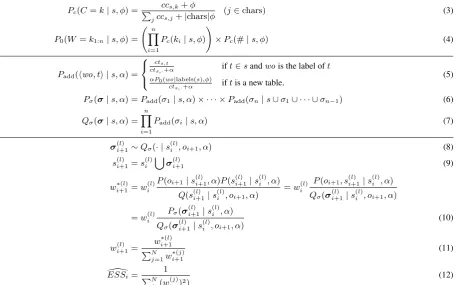
Our models are basically the unigram and bigram models described in Goldwater et al. (2009) and quickly introduced above. There is, however, an im-portant difference with respect to the choice of the base distribution that we describe in what follows. Also, our assumption about what constitutes a hy-pothesis is different from Goldwater et al., which is why we describe it in some detail.6 The mathemati-cal details are given in figure 1 while in the text, we focus on a high-level explanation of the ideas.
Pc(C=k|s, φ) =
ccs,k+φ
P
jccs,j+|chars|φ
(j∈chars) (3)
P0(W=k1:n|s, φ) = n
Y
i=1
Pc(ki|s, φ)
!
×Pc(#|s, φ) (4)
Padd(hwo, ti |s, α) =
cts,t
cts,·+α ift∈sandwois the label oft αP0(wo|labels(s),φ)
cts,·+α iftis a new table.
(5)
Pσ(σ|s, α) =Padd(σ1|s, α)× · · · ×Padd(σn|s∪σ1∪ · · · ∪σn−1) (6)
Qσ(σ|s, α) = n
Y
i=1
Padd(σi|s, α) (7)
σ(il+1) ∼Qσ(· |s(il), oi+1, α) (8)
si(l+1) =si(l)[σ(il+1) (9)
wi∗(+1l)=wi(l)P(oi+1|s (l) i+1, α)P(s
(l) i+1|s
(l) i , α) Q(s(il+1) |s(il), oi+1, α)
=w(il) P(oi+1, s (l) i+1|s
(l) i , α) Qσ(σ
(l) i+1|s
(l)
i , oi+1, α)
=wi(l)
Pσ(σ(il+1) |s (l) i , α) Qσ(σ(il+1) |s
(l)
i , oi+1, α)
(10)
w(il+1) = w ∗(l) i+1
PN j=1w
∗(j) i+1
(11)
\
ESSi= 1
PN j (w
(j) i )2)
(12)
Figure 1: The mathematical details needed for implementing the algorithm. ccs,kis the number of times characterk
has been observed in the words inlabels(s)which, in turn, refers to the words labeling (unigram) tables in model state
s.charsis the set of different characters in the language, including the word-boundary symbol#. cts,t refers to the number of customers at tabletin model states, andcts,·refers to the total number of customers ins. A segmentation
σis a sequence of word-table pairshwo, tithat indicates both which words make up the segmentation and at which table each word customer is seated. s∪σi refers to the model state that results from adding theithword-table pair
ofσ to hypothesiss, and the probability of adding this pair is given byPadd in eq. 5. s
S
σrefers to adding all word-table pairs inσtos.Qσis the proposal distribution from which we can efficiently sample segmentations, given an observationo, i.e. an unsegmented utterance, and a model states. Pσis the true distribution over segmentations according to which we can efficiently score proposals to calculate (the unnormalized) weightsw∗using eq. 10. Eq. 8 and eq. 10 can be calculated becauseQσ(σ | s, α, o) = QQ(σ(o|s,α,o|s,α)) = Qσ(σ|s,α)
Q(o|s,α) , the denominator of which can be efficiently calculated using the forward-algorithm.
4.1 The Lexical-Model
Even though Goldwater et al. found the choice of the lexical model to make virtually no difference for the performance of an unconstrained learner, this does not hold for online learners, an observation al-ready made by Venkataraman (2001). In the orig-inal model, each character is assumed to have the same probability θ0 = |characters1 | of being gener-ated, and words are generated by a zero-order (Un-igram) markov process with a fixed stopping prob-ability. In contrast, we assume that there is a sym-metric Dirichlet prior with parameterφon the
prob-ability distribution over characters:
θ∼Dir(φ) Pc(k) =θk
By integrating out θ, we get a ‘learned’ condi-tional distribution over characters, and consequently words, given the learner’s lexicon up to that point (eq. 3 and eq. 4).
In addition, we do not fix the probability for the word-boundary symbol, treating it as a further spe-cial character#that may only occur at the end of a word.7
prac-4.2 Probability of a segmentation
Since we are interested in the posterior distribution over hypotheses given unsegmented utterances, it is important to be clear about what constitues a
hypoth-esis. At a high level, a hypothesisscan be thought
of as a lexicon that arises from the segmentation de-cisions made for the observations up to this point. For example, if the learner previously assumed the segmentations “a dog” and “a woman”, its lexicon contains two occurences of “a” and one occurence of “dog” and “woman”, respectively.
More precisely, a hypothesis is a model state and a model state is an assignment of observed (or rather, previously predicted) word ‘customers’ to tables
(see section 2).8 At timek, the model states
k is the
seating arrangement after having segmented the
cur-rent observation ok given the previous model state
sk−1, where each observation is an unsegmented
string. As our incremental learner can only make additive changes to the ‘restaurant’ — no customers ever leave the table they are assigned to — the
hy-pothesis at timek+ 1is uniquely determined by the
seating arrangement at timekand the proposed
seg-mentation for observationok+1, as a segmentation
not only indicates the actual words, e.g. “a” and “dog”, but also the table at which each word should be seated (which may be a new table). Thus, going from one model state to the next corresponds to sam-pling a segmentation for the new observation (eq. 8) and adding this segmentation to the current model state (eq. 9). The formulae that assign probabilities to segmentations are given in eq. 5 to eq. 7.
5
The Particle Filter algorithm
Our algorithm is an instance of a Particle Filter, or more precisely, of the Sequential Importance Re-sampling (SIR) algorithm (Doucet et al., 2000). The idea is to sequentially approximate a target
poste-rior distributionP byN weighted point samples or
particles, updating each particle and its weight in light of each succeeding observation. Hypotheses
tical problem as we only use the model for inference, not for generation.
8The reason our description involves an explicit record of
table assignments is that this is needed for the Bigram model. While actually not needed for the Unigram case, our formula-tion can be extended to the Bigram model in a straight-forward way, given the description in Goldwater et al. (2009).
that do conform to the data gain weight, mimicking a kind of a “survival of the fittest” dynamic. No-tably, the accuracy of the approximation increases with the number of particles, a result borne out by our experiments.
At a very high-level, a Particle Filter is very sim-ilar to a stochastic beam-search in that a number of possibilities is explored in parallel, and the choice of possibilities that are further explored is biased to-wards locally good, i.e. high-probable ones.
At any given stage, the weighted particles give a finite approximation to the target posterior distribu-tion up to that point, the weight of each particle rep-resenting its probability under the approximation. Therefore, we can use it to approximate any expec-tation of the posterior, e.g. some measure of its word segmentation accuracy, as a weighted sum.
5.1 Description of the Algorithm
A formal description of the algorithm is given in Fig-ure 2 which we explain in more detail here. The
al-gorithm starts at timei= 0withN identical model
states (particles)s(n)0 , in our case empty lexicons, or
rather empty restaurants.9 At each time stepi+ 1, it
propagates each particle by sampling a segmentation
σi+1(l) for the next observationoi+1 according to the
the current model states(l)i (eq. 8) and adding this
segmentation to it, yielding the updated particles(l)i+1
(eq. 9). Intuitively, at each step the learner predicts a segmentation for the current observation in light of what it has learned so far. Adding a segmentation to a model state corresponds to adding the word cus-tomers in the segmentation to the corresponding ta-bles. As there are multiple particles, in principle the algorithm can explore alternative hypotheses, remi-niscent of a beam-search.
Not all hypotheses, however, fit the observations equally well, and as new data becomes available at each time step, the relative merit of different hy-potheses may change. This is captured in a particle
filter by assigning weightswi(l)to each particle that
are iteratively updated, using eq. 10 and eq. 11. This update takes both into account how well the particle fit previously seen data in the form of the old weight, and how well it fits the last observation in the form
9The superscript indexes the individual particles, the
of the probability of the proposed segmentation un-der the current model.
Also, the formula we use for calculating the par-ticle weights, taken from Doucet et al. (2000), over-comes a fundamental problem in applying Particle Filters to this kind of model: we are usually not able to efficiently sample directly fromP, because
P does not decompose in the way required for
Dy-namic Programming (Johnson et al., 2007; Mochi-hashi et al., 2009). The SIR algorithm, however, al-lows us to use an arbitrary proposal distributionQ for the samples. All that is needed is that we can cal-culate the true probability of each sample according toP, which is easily done using eq. 6. Our proposal distributionQignores the dependencies between the words within an utterance, as in eq. 7. This can be thought of as ‘freezing’ the model in order to de-termine a segmentation, just as in the PCFG pro-posal distribution of Johnson et al. (2007). Thus, the proposal segmentations and other quantities re-quired to calculate the weights and propagate the particles are efficiently computable using the formu-lae in Figure 1 and the efficient algorithms described in detail in Johnson et al. (2007) and Mochihashi et al. (2009). Interestingly, even though the proposal distribution is only an approximation to the true pos-terior, Doucet et. al point out that as the number of particles goes to infinity, the approximation still con-verges to the target (Doucet et al., 2000).
Resampling A well known problem with
Parti-cle Filters is that after a number of observations most particles will be assigned very low weights which means that they contribute virtually nothing to the approximation of the target distribution. This is di-rectly addressed by resampling steps in the SIR al-gorithm: whenever a quantity known as Effective Sample Size (ESS), approximated by eq. 12, falls below a certain threshold, say, N2, the current set of particles is resampled by sampling with replacement from the current distribution over particles defined by the current weights. This results in high weight particles having multiple ‘descendants’, and in low weight particles being ‘weeded out’. We experiment with two thresholds,N and N2.
6
Experiments
We evaluate our algorithm along the lines of experi-ments discussed in Pearl et al. (2011), using Brent’s
create N empty modelss(1)0 tos (N) 0
set initial weightsw0(l)toN1 forexamplei= 1→Kdo forparticlel= 1→Ndo
sampleσ(il)∼Qσ(· |s(il−)1, oi, α)
s(il)=s(il−)1S
σ(il)
calculate the unnormalized particle weightw∗i(l) end for
calculate the normalized particle weightsw(il)and calculateESS[
ifESS[ ≤T HRESHOLDthen resample all particles according tow(il) set all weights to N1
end if end for
Figure 2: Our Particle Filter algorithm.Nis the number of particles,Kis the number of examples. The formulae needed are given in Figure 1.
version of the Bernstein corpus (Brent, 1999). Un-like them, however, we see no reason for actually splitting the data into training and test sets, follow-ing in this respect previous work such as Goldwater et al. (2009) by training and evaluating on the full corpus.
6.1 Evaluation
Evaluation is done for each learner by ‘freezing’ the model state after the learner has processed all examples and then sampling a proposed segmenta-tion for each exampleofromQσ(· | s, o, α), where
s is the final model state. As we have multiple
weighted final model states, the scores are calcu-lated by evaluating each model state and then tak-ing a weighted sum of the individual scores. This corresponds to taking an expectation over the poste-rior. Note that under the assumption that at the end of learning the ‘lexicon’ no longer changes,
sam-pling from Qno longer constitutes an
approxima-tion as the intra-utterance dependencies Qignores correspond to making changes to the lexicon.
cor-rectly identified 1 of the 6 tokens and predicted a total of 5 tokens, yielding a token recall of 1/6 and a token precision of 1/5. It has also identified 2 of the 4 boundaries, and has predicted a total of 3 bound-aries, yielding a precision of 2/3 and a recall of 1/2. Lastly, it has correctly found only 1 of the 4 word types and predicted a total of 3 word types, giving a precision and a recall of of 1/3 and 1/4, respec-tively. So as to not clutter the table, we only report f-measure.
6.2 Experimental Results
There are two questions of interest with respect to the performance of the algorithm. First, we would like to know how faithful the algorithm is to the original model, i.e. whether the ‘optimal’ solution it finds is close to the ‘optimal’ solution according to the true model. For this, we compare the
log-probability of the training data each algorithm
as-signs to it after learning. Second, we would like to know how well each algorithm performs in terms of the segmentation objectives.
For comparison to our Particle Filter algorithm, we used Pearl et al.’s (2011) implementation of their proposed online learners, the DPM and the DMCMC algorithm, and their implementation of a batch MCMC algorithm, a Metropolis Hastings
sampler.10 We set the threshold for resampling toN
and N2,φto 0.02 and the remaining model
parame-ters to the values reported in Goldwater et al. (2009):
α = 20.0, ρ = 2.0 for the unigram model, and
α0 = 100.0, α1 = 3000.0, p$ = 0.5 for the
bi-gram model.11 In addition, we decided to not use
annealing for either of the algorithms to get an idea of the ‘raw’ performance of their performance and simply run the unconstrained sampler for 20,000 it-erations. While this does not reflect a ‘true’ ideal learner performance, it seems to us to be a reason-able method for an initial comparision, in particular
10The scores reported in their paper apply only to their
training-test split. We weren’t able to run the DMCMC algo-rithm for the Unigram setting which is why we omit these scores — the scores reported for the Unigram learner on a five-fold training-test split in Pearl et al. are slightly better than for our best performing particle filter but not directly comparable, and no log-probability is given.
11p$is the fixed utterance-boundary base-probability,ρis the
beta-prior on the utterance-boundary probability in the unigram model.
since we have not yet applied ideas such as anneal-ing or hyper-parameter samplanneal-ing to the Particle Fil-ter.
The particle filter results vary considerably, espe-cially with small numbers of particles, which is why we report an average over multiple runs and report
the standard deviation in brackets.12 The results are
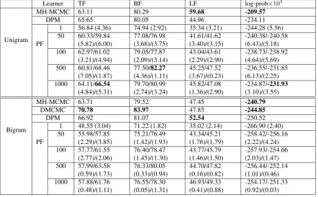
given in Table 1.
6.3 Discussion
As could be expected, faithfulness to the original model increases with larger numbers of particles — the log-probability of the training-data seems to
be positively related to N, though obviously
non-linearly, and we expect that using even larger num-bers of particles will bring the log-probability even closer to that assigned by the unconstrained learner. Also, the Particle Filters seem to work generally bet-ter for the Unigram model which is not very sur-prising, considering that “when tracking bigrams in-stead of just individual words, the learner’s hypothe-sis space is much larger” (Pearl et al., 2011), and that Particle Filters are known to perform rather poorly in high dimensional state spaces.
In the Unigram setting, the Particle Filter is able to outperform the DPM algorithm in the 1000 particle /
N
2 threshold setting, both in terms of log-probability
and segmentation scores. With respect to the lat-ter, it also outperforms the unconstrained learner in all but lexical f-measure. This is not very surpris-ing, however, as Goldwater (2007) already found that sub-optimal solutions with respect to the actual model may be better with respect to segmentation, simply because the strong unigram assumption is so blatantly wrong.
For both the models, using a resampling
thresh-old of N2 instead ofNseems to lead to better
perfor-mance with respect to both measures, in particular in the Bigram setting. We are not sure how to interpret this result but have the suspicion that this difference may disappear as a larger number of particles is used and that what may be going on is that for ‘small’ numbers of particles, the diversity of samples drops too fast if resampling is applied after each
observa-12For 1, 50 and 100 particles, we run 10 trials, for 500 and
Learner TF BF LF log-prob×103
Unigram
MH-MCMC 63.11 80.29 59.68 -209.57 DPM 65.65 80.05 44.96 -234.11
PF
1 56.84 (4.36) 74.94 (2.92) 35.34 (3.21) -244.28 (5.56) 50 60.33/59.84
MH-MCMC 63.71 79.52 47.45 -240.79 DMCMC 70.78 83.97 47.85 -244.85 DPM 66.92 81.07 52.54 -250.52
PF
1 48.55 (3.04) 71.22 (1.82) 35.02 (2.14) -266.90 (2.40) 50 55.98/57.85
Table 1: F-measure and log-probabilities on the Bernstein corpus for Pearl et al.’s (2011) batch MCMC algorithm (MH-MCMC), the online algorithms Dynamic Programming Maximization (DPM) and Delayed Markov Chain Monte Carlo (DMCMC), and our online Particle Filter (PF) with different numbers of particles (1, 50, 100, 500, 1000). TF, BF and LF stand for token, boundary and lexical f-measure, respectively. For the Particle Filter, numbers left of a ‘/’ report scores for a resampling threshold ofN, those on the right forN2. Numbers in brackets are standard-deviations across multiple runs. Numbers in bold indicate the best overall performance, and the best performance of an online learner (if different from the best overall performance).
tion.
In the Bigram setting, even 1000 particles and a
threshold of N2 cannot outperform the conceptually
much simpler DPM algorithm, let alone the DM-CMC algorithm that comes pretty close to the un-constrained learner. The increased dimensionality of the state-space may require the use of even more particles, a point we plan to address in the future by optimizing our implementation so as to handle very large numbers of particles.
Also, there is no clear relation between the num-ber of particles that are used and the variance in the results, in particular in the Unigram setting. While we are not sure about how to interpret this result, again it may have to do with the increased dimen-sionality: a possible explanation is that in the Un-igram setting, 500 and 1000 particles already allow the model to explore very different hypotheses,
lead-ing to a larger variance in results, whereas in the Bi-gram setting, this number of particles only suffices to find solutions very close to each other.
All in all, however, the results suggest that us-ing more particles gradually increases the learner’s performance. This is unconditionally true for both settings in our experiments with respect to the log-probability; while this trend is not consistent for all segmentation scores, this simply reflects that the relation between log-probability and segmentation performance is not transparent, even for the Bigram model, as is clearly seen by the difference between the DMCMC and the Unconstrained learner.
past examples for a fixed amount of time at certain intervals and can, in principle, be added to our algo-rithm, something we plan to do in the future. Also, while the performance of the DPM algorithm for the Bigram model is rather impressive, it should be noted that the DPM algorithm embodies a heuristic greedy strategy that may or may not work in certain cases. While it obviously works rather well in this case, there is no mathematical or conceptual motiva-tion for it and we can’t be sure that its performance does not depend on accidental properties of the data.
7
Conclusion and Outlook
We have presented a Particle Filter algorithm for the Bayesian word segmentation models presented in Goldwater et al. (2009). The algorithm performs competitively with other proposed online algorithms for this kind of model, and as predicted, its perfor-mance increases with larger numbers of particles.
To our knowledge, it constitutes the first Particle Filter for this kind of model. Our formulation of the Particle Filter should extend to similarly com-plex Bayesian models in Computational Linguistics, e.g. the grammar models proposed in Johnson et al. (2007) and Liang et al. (2010), and may serve as a starting point for applying other Particle Filter al-gorithms to these models, a point we want to address in future research.
Also, while the strict online nature is desirable from a cognitive point of view, for practical pur-poses variants of Particle Filters that violate these
strong assumptions, e.g. using the idea of
reju-venation that has previously been applied to Parti-cle Filters for Latent Dirichlet Allocation in Canini et al. (2009), might offer considerable performance gains for practical NLP tasks, and we plan to extend our algorithm in this direction as well.
8
Acknowledgments
We would like to thank the reviewers for their help-ful comments, and Lisa Pearl and Sharon Gold-water for sharing the source code for their
learn-ers and their data with us. This work was
sup-ported under the Australian Research Councils Dis-covery Projects funding scheme (project number DP110102506).
References
Christopher M. Bishop. 2006. Pattern Recognition and Machine Learning. Springer.
Michael R. Brent. 1999. An efficient, probabilistically sound algorithm for segmentation andword discovery.
Machine Learning - Special issue on natural language learning, 34:71 – 105.
Kevin Canini, Lei Shi, and Thomas Griffiths. 2009. On-line inference of topics with latent dirichlet allocation. In Proceedings of the Twelfth International Confer-ence on Artificial IntelligConfer-ence and Statistics.
Arnaud Doucet, Simon Godsill, and Christophe Andrieu. 2000. On sequential monte carlo sampling meth-ods for bayesian filtering. Statistics and Computing, 10:197–208.
Sharon Goldwater, Thomas Griffiths, and Mark Johnson. 2009. A bayesian framework for word segmentation: Exploring the effects of context. Cognition, 112:21– 54.
Sharon Goldwater. 2007. Nonparametric Bayesian Mod-els of Lexical Acquisition. Ph.D. thesis, Brown Uni-versity.
Mark Johnson and Sharon Goldwater. 2009. Improving nonparameteric bayesian inference: experiments on unsupervised word segmentation with adaptor gram-mars. InProceedings of Human Language Technolo-gies: The 2009 Annual Conference of the North Ameri-can Chapter of the Association for Computational Lin-guistics, pages 317–325.
Mark Johnson, Thomas Griffiths, and Sharon Goldwater. 2007. Bayesian inference for pcfgs via markov chain monte carlo. In Proceedings of NAACL HLT 2007, pages 139–146.
Percy Liang and Dan Klein. 2009. Online em for unsu-pervised models. InProceedings of NAACL 2009. P. Liang, M. I. Jordan, and D. Klein. 2010.
Probabilis-tic grammars and hierarchical dirichlet processes. In T. O’Hagan and M. West, editors, The Handbook of Applied Bayesian Analysis. Oxford University Press. Bhaskara Marthi, Hanna Pasula, Stuart Russell, and
Yu-val Peres. 2002. Decayed mcmc filtering. In Pro-ceedings of the Conference on Uncertainty in Artificial Intelligence, 2002 (UAI-02).
Daichi Mochihashi, Takeshi Yamada, and Naonori Ueda. 2009. Bayesian unsupervised word segmentation with nested pitman-yor language modeling. InProceedings of the 47th Annual Meeting of the ACL and the 4th IJCNLP of the AFNLP, page 100108.
Lisa Pearl, Sharon Goldwater, and Mark Steyvers. 2011. Online learning mechanisms for bayesian models of word segmentation. Research on Language and Com-putation, Special issue on computational models of language acquisition.