Metrics with zero and almost-zero Einstein action
in quantum gravity
G. Modanese1*
1 Free University of Bozen-Bolzano, Faculty of Science and Technology, Bolzano, Italy; [email protected]
* Correspondence: [email protected]
Abstract: We generate numerically on a lattice an ensemble of stationary metrics, with spherical
symmetry, which have Einstein actionSE ¯h. This is obtained through a Metropolis algorithm
with weight exp(−β2S2E)andβ¯h−1. The squared action in the exponential allows to circumvene
the problem of the non-positivity of SE. The discretized metrics obtained exhibit a spontaneous
polarization in regions of positive and negative scalar curvature. We compare this ensemble with a class of continuous metrics previously found, which satisfy the conditionSE=0 exactly, or in certain
cases even the stronger conditionR(x) =0 for anyx. All these gravitational field configurations are of considerable interest in quantum gravity, because they represent possible vacuum fluctuations and are markedly different from Wheeler’s “spacetime foam”.
Keywords: General Relativity; Euclidean quantum gravity; Path integral; Lattice field theory; Metropolis algorithm
1. Introduction
Among the obstacles encountered in the formulation of quantum gravity theories one can certainly mention the difficulties in the Euclidean formulation (analytical continuation to imaginary time), which is usually employed in discretized lattice versions of quantum field theory [1,2]. This problem is in turn related to the non-positivity of the Einstein action [3,4].
The two main current approaches to lattice quantum gravity, namely those of Hamber and collaborators [2,5,6] and Ambjørn and collaborators [7] take a quite radical stance in the general re-definition of 4D spacetime as a discrete quantum dynamical object. Therefore the answers given in these approaches to the issues of stability and analyical continuation are not simple to translate into familiar quantum field theory language and can be possibly understood in “entropic” terms (see for instance the discussion of the conformal instability in [2]).
The stability issue is also related, in our opinion, to one of the crucial questions in quantum gravity, particularly from a path integral point of view: among the infinite possible configurations of a void spacetime (many of which singular), why do we see on average a flat metric, and what are the most important fluctuations? Our aim in this work is not to give a general answer to this question, but only to obtain some insights in a simplified case, namely a path integral of the form
Z
d[gµν]exp
i
¯
hSE
= Z
d[gµν]exp
i
¯
h
− 1
16πG
Z
d4xqg(x)R(x)
(1)
defined in the usual metric formalism and restricted to field configurations which are time-independent and spherically symmetric. Metrics for whichSE=0 orSEh¯ clearly play an important role in this
path integral.
In previous work we have been looking for stationary non-flat metrics, which we call “zero modes of the Einstein action”, such thatR
d4x√gR=0. We found in [8–10] perturbative solutions (weak-field zero modes) with regions of opposite curvature, either in the form of dipoles or concentric shells. In
[11] we found exact non-perturbative solutions with spherical symmetry of thelocalconditionR=0
and deformations of these solutions which still satisfyR
d4x√gR=0, forming an infinite-dimensional functional space.
The sets of these classical metrics can be regarded as extensions of the so-called Einstein spaces in the Petrov classification [12], defined as the solutions ofRµν=kgµν; by weakening this condition
we can consider the conditionRµν=0,R=0 and finally
R √
gR=0. While in General Relativity it
is natural to devote special attention to the spaces withRµν= 0 (vacuum solutions of the Einstein
equations), in a path integral for quantum gravity it is natural to focus on the conditionSE=0. Note
that in usual field theories with a positive-definite action one never encounters such a distinction between the minima of the action and its zero-modes.
After finding these zero modes, however, we still do not know how much do they contribute to the path integral, unless we can evaluate it at least approximately. Working with the imaginary exponential exp(iSE/¯h)one can obtain some formal results [13], but a numerical lattice approach is
not viable. If one tries to discretize the integral and perform it numerically on Wiener paths, one only obtains wild oscillations and a confirmation of the undefined sign of the action (Sect.2.3).
So a new idea developed in this work is to explore the zero-modes on a lattice using a Metropolis algorithm of the same kind successfully employed in statistical mechanics based on the energy, with weight exp[−E/(kBT)], or in Euclidean field theories with positive-defined actions. The method
consists in starting from a metric which has zero action and is also a minimum of the action (flat space), then generate local deformations of this metric and accept them only if their action differs from zero by a quantity¯h, like in a semiclassical approximation of the Lorentzian path integral, but without any restriction to weak fields. For this purpose we use in the Metropolis algorithm the weight exp(−β2S2E),
withβ 1/¯h(a limit which formally corresponds to a very low temperature). The choice of the
squared action is the simplest one, although obviously not the only possible. Another simple choice is to use|SE|(Sect.4.1); the results are very similar, thus showing the robustness of the approach.
We start in Sect.2by laying out immediately our method for the calculation of the discretized
action. Then in Sect.3we give a short review of previous work on classical, exact zero modes of the
Einstein action. This serves as background and motivation for the present work. Sect.4contains our
results. In Sect.2we offer a comparison with other approaches to quantum gravity. Finally, Sect.6
contains our conclusions and an outlook on future work.
2. Simplified recipe for the discretized path integral
We shall consider a specific subset of metric configurations, such that the lattice action takes a simple form. Even this subset contains, however, interesting candidates as unexpected vacuum fluctuations.
2.1. Spherically symmetric spaces with constant gtt
Let us consider the set of all time-independent spherically symmetric metrics, and write the invariant interval as
dτ2=−gµνdxµdxν=B(r)dt2−A(r)dr2−r2(dθ2+sin2θdφ2) (2)
whereA(r) =grr(r)andB(r) =gtt(r)are two arbitrary smooth functions. The scalar curvature can
then be expressed as [14]
R=−Rtt B +
Rrr A +2
Rθθ
r2 (3)
where
Rtt=−B
00
2A+
B0
4A(a+b)− B0
Rrr= B
00
2B−
1
4b(a+b)−
a
r (5)
Rθθ=−1+ r
2A(−a+b) +
1
A (6)
a= A 0
A; b= b0
B (7)
If we limit ourselves to the simpler caseB=const.=1, the entire expression forRreduces to
R=−2 r
A0 A2 +
1 r − 1 Ar (8)
When we multiply this by√gand integrate ind3xand over a finite time interval(−τ,τ), we obtain
SE=− 1
16πG·2τ
Z ∞
0 dr4πr 2· −2
r q
|A|
A0 A2 +
1 r − 1 Ar (9) = τ G Z ∞ 0 dr rA0
A2 +1− 1
A
(10)
The path integral, reduced to this space, that we compute in the following, has the form
hA(r1)i=
R
d[A(r)]A(r1)eiSE/¯h
R
d[A(r)]eiS/¯h , (11)
wherer1∈[0,+∞)and we set the boundary conditionA(+∞) =1. For the moment we just trust that this makes sense and converges in spite of the oscillating factor exp(iSE/¯h), according to the original
Feynman formulation (or better thanks to it). But we shall see that this is not numerically viable and it is better to turn to a properly modified Euclidean version.
2.2. Discretized action
Let us choose units in whichG = c = h¯ = 1, and an integration timeτ = 1. We reduce the
domain ofA(r)to a finite interval(0,L)and divide it intoNparts, withδ= L/N. Discretizing the
action we obtain
SdiscrE =δ
N
∑
h=0q
|Aˆh| 2h+1
2 ˆA2
h
(Ah+1−Ah) +1−
1 ˆ
Ah !
(12)
where ˆA= (Ah+1+Ah)/2. The initial conditions areA0, ...,AN=1. The (fixed) boundary condition
isAN+1=1.
It is straightforward to see that if we change by±εone of theAhthere are only two terms in the
sum which are changed. The corresponding variation inSdiscrE can be written explicitly, but it is safer to compute it numerically by difference at every Metropolis step.
2.3. Comparison to the scalar field case and Lorentzian path integral
It is useful to make a comparison with a fieldφ(r)with classical vacuum valueφ(r) =φ0and with the usual quadratic action
Sφ= Z ∞
0 dr
h
φ0(r)2+m2(φ(r)−φ0)2
i
where we take in the followingm=1,φ0=1, so that it has the same vacuum value asA.
Let us first try to compute numerically the Lorentzian path integral, even though we know from the start that there are little chances to obtain a convergent result. We compute the quantity
hφki= R
d[φ]φkeiS/¯h R
d[φ]eiS/¯h (14)
This is not a real-valued average, but a complex “transition element”, according to the Feynman denomination. As long asS/¯h1 andeiS/¯h'1, we may expect thathφkiis approximately real and
close to 1.
We write the discretized action as
Sφdisc=δ
N
∑
h=0"
φh+1−φh
δ
2 +
φh+1+φh
2 −1
2#
(15)
with the boundary conditionφN+1=1.
Next we generateNvariables of the formφh=1+ξ,−a<ξ<a, whereξis a random number
and the amplitudeais initially very small (small deformations of the classical solution). The integrands
in (14) are evaluated in correspondence of these values of φh and the procedure is repeated for a
large number of times, averaging the results. In the limit of infiniteathis gives the so-called “Wiener
path integral”, actually an ordinaryN-dimensional integral corresponding to a path integral along
non-differentiable zigzag paths.
For small values ofathe fluctuations are small and we obtain for instance in the caseN =50,
¯
h=1 the reasonable numerical results of Tab.1.
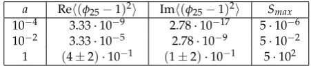
Table 1.Feynman-Hibbs transition elements computed numerically in the Lorentzian path integral (14) in dependence on the amplitudeaof the integration interval. The last column gives the maximum value of the action recorded during the Monte Carlo integration, which runs typically over 10 to 100 million random values of the setφ1, ...,φ50.
a Reh(φ25−1)2i Imh(φ25−1)2i Smax 10−4 3.33·10−9 2.78·10−17 5·10−6 10−2 3.33·10−5 2.78·10−9 5·10−2 1 (4±2)·10−1 (1±2)·10−1 5·102
The precision quickly decreases, however, when the amplitudeaincreases, and fora>1 the real
and imaginary parts ofhφkiundergo wild fluctuations even over very long runs. It appears that the
“destructive interference” effect due to the oscillating factoreiS/¯h, which in principle should lead to the cancellation of the contributions from paths very far from the classical one, cannot in practice be reproduced numerically.
Nevertheless, since the action of theφ-field is positive-defined, we can simulate a Lorentzian path
integral with the limitationSφ h¯ as a thermal system at equilibrium at a suitable temperatureT
using the Metropolis algorithm, i.e., starting from certain initial conditions (for instance the classical
vacuum valueφh=1 for anyh), making random changes of theφhand accepting them unconditionally
if the corresponding∆Sφis positive, or else with probabilitye
−β∆Sφ. If we take β= 1/(k
BT)large
enough (implying a sufficiently low temperature), the simulation will sample in an effective way all
the states withβS 1; it is possible to monitor the process by recording the maximum value ofS
attained, or better with a histogram or time-series of all values ofS. In suitable units, we shall therefore
satisfy the conditionSφ ¯h, so we are effectively sampling the configurations with an action very
close to the minimum, and we can compute in this sample averages of quantities likehφki,h(φk−1)2i,
2.4. Back to gravity: SEis not positive, then sample with S2Eor|SE|
Now let us go through the same steps for the gravitational fieldAand its path integral (11). The classical vacuum value and the initial conditions are the same: Ah=1,h =1, . . . ,N. The actionSE,
however, is not positive-defined. In the Lorentzian path integral with the Wigner paths, with small amplitudea, we can see by monitoringSEthat it changes in sign, but still it remains small in absolute
value and the results forhAikin this limit are similar to those forhφki. Whenais increased, the positive
and negative fluctuations inSEincrease, adding to the noise coming from the factoreiS/¯h. It would not
make sense to pass, like forφ, to a Metropolis simulation based onSEin order to obtain the “thermal
sampling” of the region withSE¯h. We can do, however, the Metropolis sampling withS2E, using
the probabilitye−β2∆S2E. As with theφ-field, we can check that during the runs the values ofS
Eremain
very close to the minimum and we can compute the averages ofhAki,h(Ak−1)2i. The results are
given and discussed in Sect.4, and are very different from those for φ! Large deviations from the
classical valuesAk=1 are observed.
Is is important, at this point, to consider the following natural objection: minimizingS2
Eis not the
same as minimizingSE, because∆(S2E) = 2SE∆SE, so that a classical theory based on the actionS2E
has more solutions than one based onSE. Actually, the additional classical solutions are just the zero
modes discussed previously, for whichSE =0. In order to reply to this objection we note that:
(1) The configurations withSE ¯hobtained from the Metropolis algorithm withS2Eare very
different from the classical zero modes ofSE. Therefore such configurations cannot originate from the
spurious minimum ofS2EatSE = 0 and it appears that, ironically, the only use of the classical zero
mode solutions is for making sure that they are irrelevant (probably due to entropic or phase-space
reasons). (2) As a further check, we have run the algorithm also with a probability based on|SE|.
Results are very similar (see Sect.4.1). Although the absolute value looks a bit cumbersome and was
not our first choice, it has the advantage that no spurious stationary points are introduced.
3. Classical, exact zero modes
In this Section we give a short review of our previous work on classical, exact zero modes of the Einstein action. These are metrics for whichSE=0 (SEis defined in eq. (1)), or in other words metrics
whose scalar curvature has vanishing integral.
In perturbation theory, one can obtain such zero modes defining, at a purely mathematical level, some suitable unphysical sources and solving the linearized Einstein equation for these sources. The Einstein equations with sourceTµνobtained from the Einstein action are, as usual
Rµν−1
2gµνR=−
8πG
c4 Tµν (16)
By contraction withgµνone obtains
R= 8πG c4 g
µνT µν=
8πG
c4 T
ρ
ρ (17)
Therefore if we define a source such that
Z d4x
q
g(x)Tρρ(x) =0 (18)
its field will be a zero mode. If the source is static, we can suppose for simplicity that only the
T00 component is non vanishing. The factor√gg00 can be expressed in function ofT00through the
Feynman propagator and the conclusion is that
q
Therefore the action can simply be rewritten, for that source, as
SE=−1
2
Z
d4xT00(x) +o(G2) (20)
and in order to haveSE=0 at this level of approximation it is sufficient to choose an unphysical source T00(x)of the form of a mass dipole, or one with spherical symmetry, with two concentric mass shells of opposite sign [9].
Turning to the strong-field case, in [11] we used a virtual source method to search for zero modes of the action. In the context of wormhole physics [15] this method is also called “reverse solution of the Einstein equations”; it consists in finding a source which generates a metric with some desired features. The goal here would be to find zero modes with curvature polarization, namely having two regions with positive and negative scalar curvature such that the total integral of√gRis zero. However, this turns out to be impossible, because the source must also satisfy independently the Bianchi identities, and the two conditions are found to be incompatible beyond the linear approximation.
Still there exist in the strong-field case a set of static and spherically symmetric zero modes without polarization. In fact the condition that the integrand of the action (10) be identically zero can be written as an ordinary differential equation in the unknownA(r):
rA0(r) A2(r) +1−
1
A(r) =0 (21)
It is straightforward to check that the solutions of this equation are scale invariant, i.e., ifA(r)is a solution, then alsoA(kr)is a solution, for any positivek. The non-singular solution such thatA(r)→1
whenr→∞is
A(r) = r
r+µ, µ≥0 (22)
One can check that this solution has for largerthe same form as a Schwarzschild metric with mass−µ.
It is regular everywhere, monotonically increasing fromA(0) =0, and equal to 12whenr=µ.
Finally one can define small periodic deformations of the zero modes (22) which still have null integral, although they do not haveR=0 everywhere (see details in [11]).
In conclusion, there exist for the Einstein action weak classical zero modes of the polarized kind and strong field zero modes which are not polarized. We have discussed analytically the possible role
of these modes in the path integral in [13]. In the next section we shall see what happens in strong
field lattice simulations.
4. Results of the quantum simulations
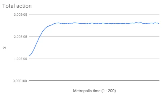
The best choice of the parameters in the Metropolis simulation for attaining thermal equilibrium is found to beε=10−6,β=1013. With this choice the total actionSEreaches quickly a small positive
value of the order of 10−5(Fig.1). A typical run includes 200 time steps, each with 5·106local “spin flips” of the variablesAh. The average values ofAhare computed in the second half of the run, after
equilibration. Typical figures for other averages of interest arehSi=2.6·10−5andhe−β2∆(S2)i=0.98
(acceptance ratio for changes with∆(S2)>0).
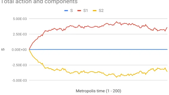
Fig.2 shows that the componentS1 of the action (the one given by the sum in the interval
0<r<L/2, i.e., with indexhfrom 1 toN/2) is positive, and vice-versa for the componentS2. From
Fig.3we see that in the same interval the metric A(r) is approximately constant, sayA ' 1−χ
(0<χ1), and conversely in the interval betweenL/2 andLwe haveA'1+χ.
In the expression (10) for the action we observe that if Ais constant in an interval, then the integrand reduces to(1− 1
A). By replacingA'1±χ, we find that the integrand is approximately
equal to−χin the left interval and to+χin the right interval, i.e., it is opposite to the values ofS1and
Metropolis time (1 - 200)
S
0.00E+00 1.00E-05 2.00E-05 3.00E-05
Total action
Figure 1.Values of the action measured during a typical Metropolis run with inverse temperature
β = 1013. An equilibrium value of the order of 10−5is attained (all quantities in units such that ¯
h=c=G=1; interval lengthL=1, number of sub-intervalsN=100).
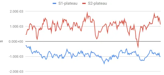
This means that the main contributions to the action do not come from the “plateaus” with constant metric (Fig.4), but from the “steps” atr=0,r=L/2 andr=L, whereRcannot be estimated as easily as in the plateaus. It is mainly the right combination of steps which makes the action vanish. Note that these steps build up spontaneously and in a reproducible way in the thermalization algorithm from billions of random flips of the discretized variablesAh.
The occurrence of one step exactly at the middle of the interval(0,L)is most likely an artifact of
the discretization (and remember that physicallyLmust tend to infinity). Still a physical phenomenon
of polarization between regions withR<0 and regions withR>0 clearly emerges from these results. Beingrthe radial coordinate of a spherical configuration, the two polarization regions are actually one
sphere and one spherical shell around it. SinceRhas opposite sign to the integrand of the action, we
conclude that in this class of vacuum fluctuations the inner region hasR<0 and the outer region has
R>0.
For comparison with the exact, classical zero modes of Sect.3(with SE = 0) we recall that
polarized zero modes are obtained in the linearized approximation, but they do not survive in strong field. Polarized zero modes in strong field appear thus to be present, and entropically dominant, only under the weaker conditionSE¯h.
4.1. Results with transition probabilityexp(−β∆|SE|)
As mentioned in Sect.2, simulations have also been performed with a transition probability based on|SE|, as an alternative toS2E. With parametersε=10−6,β=109one obtains results very similar to
those those with probability exp(−β2∆S2E)and parametersε=10−6,β=1013(Figs.1,2; the relation
between the values ofβin the two cases is not obvious, sinceεis also involved). Again we observe in
the simulation a positive action which increases until it reaches a value of the order of 10−5and then
stays approximately constant, while the polarized componentsS1andS2undergo small oscillations
around values of the order of 10−3.
With a tenfold increase in “temperature” (β=108) some different field configurations are obtained,
which are quite interesting for our purposes (Fig.5). After a moderate growth to the magnitude 10−4as before, the action returns very close to zero (|S| ∼10−9, with oscillations of both positive and negative
sign); in the meanwhile, the polarized componentsS1andS2(Fig.6) are larger by approximately 8
magnitude orders, apparently resulting from a very efficient compensation mechanism. Unlike in the
previous case, however, the componentsS1andS2do not appear to reach an equilibrium value but
Metropolis time (1 - 200)
S
-5.00E-03 -2.50E-03 0.00E+00 2.50E-03 5.00E-03
S S1 S2
Total action and components
Figure 2.ComponentsS1andS2of the action for the same run of Fig.1.S1is given by the sum from 1 toN2, i.e. on the left half of the interval.S2is given by the sum fromN2 +1 toN, i.e. on the right half. BothS1andS2are much larger, in absolute value, than the total action. Since the sign ofRis opposite to that of the localS, we conclude that the inner part of the metric has negative curvature and the outer shell has positive curvature. The total integral of the curvature is small and negative.
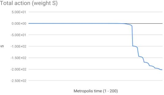
Finally, it is interesting to note that if we make simulations simply with probability exp(−βSE),
disregarding the problem of the indefinite sign ofSE, then with very low temperature (β =109or
more) one still obtains a positive growth ofSto∼10−5followed by stabilization, but going to smaller
βone observes a collapse of the action to large negative values (Fig.7). The corresponding metric
shows large deviations from flat space.
5. Comparison with other approaches
A fundamental reference point for the understanding of non-perturbative quantum gravity (QG) in the path integral approach is in our opinion the work of H. Hamber, contained in several seminal
papers starting from 1984 and summarized in the book [2] and in a few review articles. Among the
latter we can mention one from 2009 [5] and the very recent article appeared in this same Special Issue
[6], containing recent results on the quantum condensate which appears to be present in the vacuum
state of QG.
Hamber regards non-perturbative quantum chromodynamics (QCD) as a possible model for
QG, though with some important differences. In particular, in QG the cutoff or lattice spacingl0of
the discretized theory remains implicitly present in the physical value ofG, and there exists another
dynamically generated scaleξ, the correlation length of the curvature. A meaningful lattice limit is
obtained whenξl0. Although the magnitude ofξis not directly related to the value ofG, it signals
how close the bareGis to the fixed point valueGc.
These statements refer to the renormalization group analysis and to the scaling analysis in dependence on the cutoff that is necessary in order to find the correct continuum limit of lattice field theories [1], and which in this paper has not yet been performed, except for noting the scale invariance of the classical zero modes.
Actually, in our approach we do not admit the very general scale invariance considered by
Hamber, according to which the metric can undergo transformations of the formg0µν = ωgµν. We
assume that the metric is always asymptotically equal to the flat metricηµν, and so in our simulations
the componentA(r) =grr(r)has always boundary conditionA=1 at larger. This is also because
we do not have a cosmological term in the action. Hamber, on the contrary, starts from an action
containing a bare cosmological constantλ0and looks for a mechanism of dynamical generation of
r=delta*h; h=1,...,100
A
9.00E-01 9.50E-01 1.00E+00 1.05E+00 1.10E+00
Metric component A vs. discretized radius
Figure 3.Metric componentA=grras a function of the discretized radiusr =δh(δ=L/Nis the lattice cutoff). The condition at the right boundary isA=1.
Metropolis time (1 - 200)
S
-2.00E-03 -1.00E-03 0.00E+00 1.00E-03 2.00E-03
S1-plateau S2-plateau
Action contributions of metric plateaus
Figure 4.Action contributions from two metric “plateaus” where the metric is approximately constant. The contributionS1−plateaucomes from the inner region with 30≤h≤40. The contributionS2−plateau comes from the outer region with 60≤h≤70. Note that the sign ofS1−plateauis opposite to the sign of S1, and the same holds forS2−plateauandS2.
results are compatible with this fact, since the vacuum fluctuations we find have average negative scalar curvature, such to compensate a positiveλ0and bring the system closer to flat space.
Further enlarging the picture, it should be mentioned that according to Hamber the large-scale
average hRi in pure QG is not zero but equal to 1/ξ2. Therefore ξ is related to a gravitational
“condensate”, physically represented by the observed cosmological constant. This establishes a very
interesting link between QG and cosmology [6].
Other possible approaches to the problem of the true ground state in quantum gravity are those of Preparata and collaborators [16] and of Garattini [17]. Both are based on a Hamiltonian formulation. Classical wormhole metrics with spherical symmetry are taken as candidates for the ground state (with lower energy than flat space) and the spectrum of the quantum excitations with respect to this
background is computed. In Ref. [16] a “gas of wormholes” is then considered, as macroscopic limit,
Metropolis time (1 - 800)
S
-5.00E-05 0.00E+00 5.00E-05 1.00E-04 1.50E-04 2.00E-04
Total action (weight |S|, higher temperature)
Figure 5.Total action with probabilitye−β|S|and inverse temperature
β=108. It reaches a positive maximum value of the order of 10−4and then decreases to 10−9.
Metropolis time (1 - 800)
S
-2.00E-01 -1.00E-01 0.00E+00 1.00E-01 2.00E-01
S1 S2
Action components (weight |S|, higher temperature)
Figure 6.ComponentsS1andS2of the action for the same run of Fig.5. They are about 8 magnitude orders larger than the total action.
both approaches, strong quantum fluctuations are found to occur only at the Planck scale. In contrast, the action zero modes of [11] occur at any scale.
6. Conclusions and outlook
The difficulties encountered in the formulation and numerical simulation of lattice quantum gravity are manifold. This is certainly to be expected, since in quantum gravity the spacetime lattice itself takes part to the dynamics. In this general context our present contribution is quite limited, also because we consider only time-independent metrics with spherical symmetry. Nevertheless, we have been able to single out some phenomena which occur in the nonperturbative lattice dynamics and can perhaps be present under less specific circumstances. Such phenomena are quite intuitive from the physical point of view. The idea of zero modes of the action with polarization into regions of positive and negative scalar curvature, already explored at the perturbative level, is confirmed under strong field conditions.
More in detail, we can summarize our previous and present results as follows:
1. Exact zero modes (SE =0) with curvature polarization exist in the weak field approximation.
Metropolis time (1 - 200)
S
-2.50E+02 -2.00E+02 -1.50E+02 -1.00E+02 -5.00E+01 0.00E+00 5.00E+01
Total action (weight S)
Figure 7.Total action with probabilitye−βSand inverse temperature
β=108. The system is clearly unstable with respect to negative fluctuations of the action.
3. Quantum zero modes (SE¯h) of any strength are predominantly of the polarized kind.
The “trick” of weighing the configurations in the path integral withe−β2S2E (ore−β|SE|) instead of
e−βSE, in order to avoid the problem of the indefinite sign ofSE, does not seem to be a weak point of the argument. What is still missing is a scaling analysis of the results, which will be presented in a forthcoming work.
A further extension of the results could be obtained by varying in the path integral not only the metric componentgrr, but alsog00. From the analytical point of view this looks intractable, but in the numerical code it should not make a big difference, except for doubling the number of degrees of freedom and complicating the expression of the discretized action.
Finally, an open question is what average physical quantities can be defined and measured in this kind of simulations, besides the local curvature and metric, which show the occurrence of the polarization phenomenon but not its possible consequences.
Acknowledgment - This work was supported by the Open Access Publishing Fund of the Free University of Bozen-Bolzano.
1. Zinn-Justin, J.Quantum field theory and critical phenomena; Clarendon Press, 1996.
2. Hamber, H.W.Quantum gravitation: The Feynman path integral approach; Springer Science & Business Media, 2008.
3. Wetterich, C. Effective nonlocal Euclidean gravity. General Relativity and Gravitation1998,30, 159–172. 4. Modanese, G. Stability issues in Euclidean quantum gravity.Physical Review D1998,59, 024004. 5. Hamber, H.W. Quantum gravity on the lattice.General Relativity and Gravitation2009,41, 817–876. 6. Hamber, H.W. Vacuum Condensate Picture of Quantum Gravity. Symmetry2019,11, 87.
7. Ambjørn, J.; Görlich, A.; Jurkiewicz, J.; Loll, R. Nonperturbative quantum gravity. Physics Reports2012, 519, 127–210.
8. Modanese, G. Virtual dipoles and large fluctuations in quantum gravity.Physics Letters B1999,460, 276–280. 9. Modanese, G. Large “dipolar” vacuum fluctuations in quantum gravity. Nuclear Physics B2000,
588, 419–435.
10. Modanese, G. Paradox of virtual dipoles in the Einstein action. Physical Review D2000,62, 087502. 11. Modanese, G. The vacuum state of quantum gravity contains large virtual masses. Classical and Quantum
Gravity2007,24, 1899.
13. Modanese, G. Anomalous Gravitational Vacuum Fluctuations Which Act as Virtual Oscillating Dipoles. In Quantum Gravity; IntechOpen, 2012.
14. Weinberg, S.Gravitation and cosmology: principles and applications of the general theory of relativity; Wiley New York, 1973.
15. Lobo, F.S.; Visser, M. Fundamental limitations on ‘warp drive’spacetimes.Classical and Quantum Gravity 2004,21, 5871.
16. Preparata, G.; Rovelli, S.; Xue, S.S. Gas of wormholes: a possible ground state of quantum gravity. General Relativity and Gravitation2000,32, 1859–1931.