2642
D
YNAMICS OF AN
SI
MODEL WITH TIME DELAY AND
DIFFUSION
M.Sridevi , B. Ravindra Reddy
Abstract: This work presents on model of Susceptible and an infective (SI) with saturated incident rate along with this latent period has been investigated. The stability of the disease-free and endemic equilibrium for the model with and without delay is analyzed. The existence of Hopf bifurcation with time delay as the bifurcation parameter is studied. The effect of the spatial diffusion on the dynamical system is presented. To support the analytical results from this work introduced numerical simulations with various numerical values have been used and tested
Index Terms: Logistic growth, saturated incidence, delay, stability, Hopf bifurcation, diffusion.
—————————— ——————————
1.
INTRODUCTION
Mathematical models have been utilized to understand and predict the spread of disease, investigate transmission and control of diseases. K. Hattaf.et.al [1] studied the models without time delay which represented the dynamics of contagious diseases. However to reveal the dynamical aspects of models that depend on the past history of systems, time delays are incorporated in the systems as given by J. Zhang.et.al [2]. Delays can be destabilizing the original stable equilibrium in the epidemic models which lead to periodic solutions and the Hopf bifurcation as proposed by K. Hattaf.et.al [3]. In case of infectious diseases, the individuals are unable to transmit the disease immediately the moment they get infected. These individuals take a period of time to show symptoms of disease like in AIDS, rabies and so on. Mathematically it is viewed as time delay. Incorporation of delays in contagion models depicts them to be more prudent by allowing the representation of the effects of disease latency or immunity [14]. Y.Kuang [6] proposed that delay reflects not only the changes of‗t‘ moment state but also some other factors before the‗t‘ moment state. Many authors have also incorporated the incidence rate to examine the infectiousness increasing through the infected individuals which are having contact with susceptible. The saturated incidence rate of the form βSI/1+αI or βSI/1+αS was formulated as the crowding effect of infective or change in behavior of susceptible. The saturated effect of factor stems from epidemic control. This saturated incidence rate was employed by Capasso and Serio in 1978 [4]. An SIR model with a nonlinear incidence rate was studied by Ruan et.al. [5]. ―A Hepatitis B infection model with viral delay, saturation response and cure of infected cells‖ was studied by Karuna.et.al. [12]. Wang et.al [10] analyzed a SIR vector disease model with incubation time delay. The epidemiological models are precisely affected by space due to the localized environment of transmission or other individual organisms. These are scattered in their spatial region and interact with the typical environment such as physical structure, climate as given by W.Wang.et.al. [11]. Author name: M.sridevi, Asst.professor Department of Mathematics, CMR college of Engineering and Technology, Hyderabad, Telangana state, India.
The spatial contagious model is a proper tool to investigate the basic mechanisms of complex spatiotemporal epidemic dynamics. Reaction-diffusion equations are used to illustrate the spatiotemporal dynamics. M. Liu, and Xiao [7] analyzed the models based on the ordinary differential equations, are always under some assumption of homogeneous connectivity of each individual and homogeneous infectivity. Here the total population is divided into independent classes, which are closed compartments. These are large compartments in size. The epidemic model with diffusion describes the transmission of disease. G. Quan Sun [8] described that time and space is also useful to investigate the process of spread of disease. In diffusion model some authors found that the wave fronts in epidemic. M.E .Lotfi et.al [9] examined the spatiotemporal periodic solutions can occur in the epidemic model with spatial diffusion. G.Ranjith kumar et.al [13] analyzed the Hopf bifurcation of SIR model with time delay.
In this paper we discussed the equilibrium points‘ existence and their stability with and without delay and local Hopf bifurcation existence. Furthermore, we investigate how populations‘ diseases transmit in both space and time which can enhance the understanding of epidemic features of disease in the populations.
2. MATHEMATICAL MODEL
In many cases, infectious diseases are not immediately transmitted but undertake a certain period of time viewed as delay before the infection spreads to others. In this paper we incorporated a saturated incidence rate to a delayed SI model and considered the system as
1
1
( )
(1 )
1
( )
( )
1
d S S S I t
r S S
d t K S
d I S I t
I
d t S
(1)
Where S t( ), ( )I t be susceptible and infected population, is rate of transmission, is natural death rate, r is rate of intrinsic birth, K is susceptible carrying capacity, is disease death rate and is time delay. 1 is saturated factor.
_______________________
2643
3. STABILITY ANALYSIS OF THE SYSTEM
Equilibrium points from the system are specified by * 1 ( ) S When1( )
* 1 1
1
( ) ( ) ( )
2
[ ( )]
K r K K r r K
I K
The basic reproductive ratio is specified by
1 0 1 1K r K
r K K
R
3.1 DISEASE FREE EQUILIBRIUM AND ITS STABILITY
Disease Free Equilibrium (DFE)
1 ( ) , 0
K E r r
if 1
0 R
locally asymptotically stable and unstable when 1 0
R .
Case (i): when there is no delay
Jacobean matrix of the system at E1
S*, 0
is1 1 * * 2 * 1 *
0 ( )
* 1
r S S
r e S J S e S
K
In the absence of delay characteristic equation is *
2r S r
K
1 * ( ) * 1 S S
0 (2) * 2 , 1 r S r K
1 * 2 * 1 S S .At disease free equilibrium * ( ) , S r r
K
( ) , 1 r 0 2 If
1 ( ) ( ) 1( )
K r K K r K r
( ( ) )
1
( ) ( 1)
k r
k r k
1 0 R
i.e., When r and 1 0
R then equation of characteristic (2) has negative roots.
Thus DFE is locally asymptotically stable for 1 0
R and when 0
Case (ii): when 0,
Characteristic Equation is * 2r S r
K
1 * ( ) * 1 S e S
0 (3)
We assume that the root of equation
i
* 2 0 , r S r
K
1 *( ) 0
* 1 S i i e S
(4) At1 ( ) , 0
E r r K
1 (r )
another
root i must satisfy
Where r and
0
R less than one, there is no positive real root of .
At
1 ( ) , 0
E r r K
the system is asymptotically stable while r and
0 1
R ; and it is unstable when 1 0
R .
3.2 ENDEMIC EQUILIBRIUM AND ITS STABILITY
Case (i): In presence of delay
Jacobean matrix at Endemic Equilibrium (EE) is given by
* *
2( , )
2644
1 1
1 1
* * *
2
* 2 * (1 ) 1
* *
( ) * 2 *
(1 ) 1
r S I S
r e S S J I I e S S K (5)
Characteristic equation is given by
1 1
1
* * * 2 * * 2
( ) 0 3 * 2 *
* (1 ) 1
1
rS I S S I
r e e
S S S K (6)
0 1 0 1
2
( ) 0
P P e Q Q
(7) where 0 1 * * 2 2 * 2 (1 )
r S I
P r S
K
, 1 1 * * 2 ( ) ( ) ( ) ( ) * 2 (1 )r S I
P r S K 0 1 * , * 1 S Q S 1
1 1 1
* 2 *
2
* * *
1 (1 ) 1
r S r S S
Q
S K S S
When 0, Characteristic equation becomes
0 1 0 1
2
( ) 0
P P Q Q
(8)
When 1
0
R we have 0
0 0 ,
P Q and
1 1 0
P Q By Routh-Hurwitz criteria all roots of characteristic equation (8) are real and negative or complex conjugates with negative real parts.
Hence system (1) without delay is locally asymptotically stable
when 1
0
R
Case (ii) If
0 then there exists a positive0
such that characteristic equation (7) of the system has roots
, 0
i
(purely imaginary) Put i in equation (7)
0 1 0 1
2
( ) ( c o s s in ) 0
P i P Q i Q i
(9) While separating real & imaginary parts
1 0 1
0 0 1
2
s i n c o s
s i n c o s s i n
P Q Q
P Q Q
(10) Squaring & adding we get
0 0 1 1 1
4 2 2 2 2 2
(P Q 2P ) (P Q ) 0
(11)
If
0 0 1
2 2
(P Q 2P ) 0 and
1 1
2 2
(P Q ) 0then the equation (11) has no real root.
Thus for all
0 real parts of all Eigen values are negative. Hence EE is asymptotically stable for the following conditions.a R) 0 1
0 0
)( ) 0 ,
b P Q (P1 Q1) 0
(12)
0 0 1 1 1
2 2 2 2
) ( 2 ) 0 , ( ) 0
c P Q P P Q
When i0 at 0 the roots of equation (6) has pair of purely imaginary, there exists unique +Ve 0 satisfying equation (9) and there is some +Ve 0, if
2 2
1 1
P Q is –Ve From (8)
k
corresponding to
0
can be obtained
1 1 0 0
0 1
2 2
( ω - P ) - P Q ω
1 -1 2 n π
τ = c o s +
k 2 2 2
ω0 Q ω + Q ω0
Q
(13)
4. HOPF BIFURCATION
From the above results we have the following: Assume that
0 1
R then there exists +Ve
0such that the below solving result holds.a) If
0
0 then the system has locally asymptotically stable at E2.
b) If
0
a periodic orbit exists in the small neighbour of EE then system carry out a Hopf bifurcation.
We have to check transversal condition for the complex Eigen values of E2 at .
0
From (8), we have
0 1
0 0 1 0
( )
2 ( )
Q Q e
d
d t P Q Q e Q e
0 0 0 1 0 1 1 2
2 ( )
( )
P Q
d
d t P P Q Q
2645 0 0 0 1 0 1 2 1 0 R e 2 ( )
0 0 0 0
i P Q
i Q Q i P iP 0 0 0 1 0 1 2 1 0 2 ( )
0 0 0 0
i P Q
i
Q Q i
P iP
0 0 1 0 1
2 2 2
2 ( ( 2 )
0
2 2 2
0
P Q P
Q Q
Under this condition
0 0 1
2 2
(P Q 2P) 0 , this shows
0
R e ( )
0
i
d
d t
Transversal condition exists & Hopf bifurcation also occurred at
0, 0
5.
DIFFUSION
INSTABILITY
The stability of the system (1) without delay has been examined in the presence of diffusion.
1 1 2 (1 ) 2 1 2 ( ) 2 1 I
S S S I S
r S S D
S
t K S x
I S I
I D I
t S x
(14)
With Neumann boundary conditions
lim lim 0 , lim lim 0
x x x x
S S I I
x x x x
For a spatially homogeneous solution
* *
,
S I where S*and
*
I satisfy the system.
For x[ 0 , ]l andt[ 0 ,) this system (14) is considered This system is built with non negative constant diffusion coefficients D ,D
I S and by applying the Neumann boundary
conditions.
( 0 , ) ( , ) ( 0 , ) ( , ).
Ix t Ix L t Sx t Sx L t
To examine the Turing instability of the system (14), we derive the Jacobean matrix of linearization at the EE.
2
2
F k F
G G k
D
I
S S
J
d iffu s io n
D I I S (15) (15) Where 1 * * 2 * 2 (1 ) F
r S I
r S k S 1 * * 1 F S I S 1 * * 2 (1 ) G I S S 1 * ( ) * 1 G I I S
Characteristic Equation of (15) is shown by
2 0 2 F F G G D k I S S D k I I S (16)
Trace is denoted byN k( 2) and determinant is denoted
byM (k2)
where N(k2) (G F ) (D D )k2
I S I S
and
2 2 2
( ) ( ) ( ) G
M k F D k G D k F
I I I
S S S
If the diffusion coefficients are zero, then the model (14) turns out to be a system of ODE, and follow the same rules as of the ODEs. i.e., to say that the system is asymptotically stable when trace is less than zero and determinant is greater than zero at the positive equilibrium
* *
2 , .
E S I
The Trace and the determinant of (16) in the absence of diffusion coefficients are
(F G ) 0 & (F G F G ) 0
I I I
S S S
11 1
2
( ( ))
( ( ) 0
( )
F
r
G I I
I S K
1
2
( ) ( )
0
F G F G
I I S S
Thus system (14) is locally asymptotically stable.
2646 (14) are
2 2
( ) 0 , ( ) 0
N k M k .N k( 2) 0 is always negative
(F G )
I
S is negative.
2 4 2
( ) ,
M k a k b k c M (k2) is a quadratic function
of k2.
Here , F G
S
a D D b D D
I I I
S S
and c G F G F
I S S I
If 2 & 2
1 2
l l are the real roots ofM (k2) 0.
2 2 2
[ , ]
1 2
k l l
We conclude that Turing instability arise if
0
G F
D D
I I
S S and
2 ( )
G D D F D D G F G F
I S I S I S I S S I (17)
Theorem: If N k( 2) 0 ,M (k2) 0 then the EE of the system with diffusion is stable and unstable whenM (k2) 0.
6. NUMERICAL SIMULATION
For the above said and mentioned analytical methods, the observations and demonstrations of the same for various numerical examples, different level values of the parameter and other parameters for the system(1) are used as shown like this r=2.5; k =80; =0.0945; =0.0002; =0.966; =0.058. System
1 has unique positive equilibrium at
2 1 0 .8 5 9 5, 0 .1 5 8 4
E andR0 1 .9 0 9 9, the time
delay
0 0 .5 1 2 3
. It is identified from (1) that is less than 0 equilibrium point is asymptotically stable, when passes through o then EE loses its steady state and periodic solution bifurcate from E2 , this is shown below in figures (1a),(1b), (2a),(2b), &3(a),3(b).
Fig.1a
Fig. 1b
Trajectories and phase graphs of system (1) as shown when 0 .5 1 2 3
0 0 .2
2647
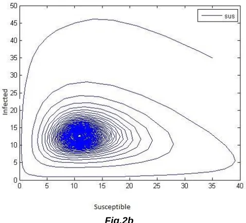
Fig.2b
Trajectories and Phase graphs of system (1) as shown when
0 0 .5 1 2 3
Fig.3a
Fig.3b
Trajectories and phase graphs of system (1) as shown when 0 .5 1 2 3
0 0 .9
Figure (4a) &Fig (4b): For the parameter values r=2.5; =0.9; k=10; =.091;
=0.99; =0.921; Dx= 0.03; Dy = 0.09; the oscillations illustrating the system (14) with space and time.
Fig.4a
Fig. 4b
7. CONCLUSION
2648 stability and then Hopf bifurcation arises at E2 From the
observations of the simulation results it is clearly shown in the figure3 (a) &3(b) that is the observed instability in the system (14) is of diffusion driven under the conditions of equation (17) hence, the stability behavior of the equilibria has been effected by the spatial diffusion with special constant coefficients. This model exists for diseases of kind influenza. The analytical methods are illustrated by the numerical simulations.
REFERENCES
[1] K.Hattaf, A.Ali lashari, Y.louartass, N .Yousfi, ―A Delayed SIR Epidemic Model with general incidence‖ Electronic Journal of QualitativeTheorey of Differential equations. No.3, pp.1-9, 2013.
[2] J. Zhang, Z. Jin, J.Yan, G.S un ―Stability and Hopf bifurcation in a delayed competition system‖, Nonlinear Analysis., vol.70, pp.658-670, 2009. [3] K. Hattaf, G..Zaman, A. Ali lashari ―A delay
differential equation model of a vector borne disease with direct transmission‖, International journal of Ecological Economics&Statistis, vol.27, Iss.4,2012
[4] V .Capasso, G .Serio, ―A generalization of the Kermack-Mckendrick deterministic epidemic model‖, Math. Bioscience, vol. 42 pp. 65-81, 1978. [5] S. Ruan and Wang. ―Dynamical behaviour of an epidemic model with a nonlinear incidence rate‖, Journal of Differential Equation, vol. 188, pp.135-163, 2003.
[6] Y. Kuang. ―Delay Differential Equations with Applications in Population Dynamics‖, Academic Press, New York, 1993.
[7] M. Liu and Y. Xiao, ―Modeling and Analysis of Epidemic Diffusion with population Migration‖, Hindawi Journal of Applied Mathematics, vol.2013, pp.583648-583655, 2013.
[8] G. Quan Sun, ―Pattern formation of an epidemic model with diffusion‖, vol.69, Nonlinear Dynamics, 2012, pp. 1097-110.
[9] M. Lotfi , K. Hattaf, , N .Yousfi, M. Maziane, ―Partial Differential Equations of an Epidemic Model with Spatial Diffusion‖, International Journal of Partial Differential Equations, vol. 2014, pp.186437-186442, 2014.
[10]J.J.Wang., J.J. Zhang, ―Analysis of an SIR model with bilinear incidence rate‖, Nonlinear Analysis of Real word Applications., vol. 11, pp. 2390-2402, 2010,
[11]W .Wang, Y .Cai, M .Wu, K.Wang, Z .Li, ―Complex dynamics of a reaction–diffusion epidemic model‖, Nonlinear Analysis of Real world Applications, vol.13, pp. 2240–2258, 2012.
[12]B.N.R. Karuna ,K. Lakshmi Narayan , B. Ravindrareddy, ―Stability Analysis of an HBV Model with Delay in viral production‖, International Journal of Ecology &development, 2010, vol.33,Iss.4, 2018.
[13]G.Ranjithkumar,K.LakshmiNarayan,B.RavindraRe ddy, ‖Stability and Hopf bifurcation Analysis of SIR Epidemic model with Time delay‖,Vol.11, No.3, ARPN Journal of Engineering & Applied
Science,2016.