Division I
AN ORIGINAL FLOW RULE FOR STRAIN-SPACE MULTI-SURFACE
SAINT-VENANT PLASTICITY MODEL
Corado Ningre1, Guilhem Bles2, Ali Tourabi3, Didier Imbault4
1
PhD Student, Univ. Grenoble Alpes, CNRS, Grenoble INP, 3SR, F-38000 Grenoble, France
2
Associate Professor, ENSTA Bretagne, FRE CNRS 3744, IRDL, F-29200 Brest, France
3
Associate Professor, Univ. Grenoble Alpes, CNRS, Grenoble INP, 3SR, F-38000 Grenoble, France
4
Associate Professor, Univ. Grenoble Alpes, CNRS, Grenoble INP, 3SR, F-38000 Grenoble, France
ABSTRACT
The one-dimensional Saint-Venant model can reproduce the elastic-plastic uniaxial behavior of metallic materials. A three-dimensional extension of this model is proposed, to simulate the cyclic elastic-plastic multiaxial behavior for complex loading paths. A multi-surface model is obtained and an original flow rule, defined in the strain space, is considered. This model has been implemented in a commercial finite element code. The model response is investigated for different loadings and compared to experimental data from the literature. The model showed accurate response in the multiaxial case of tension-torsion experiments.
INTRODUCTION
The discrete generalized Saint-Venant model has been extended to the pure hysteresis continous model by Persoz (1960), and has been studied in a more complete way by Guélin (1980). This model can reproduce the typical elastic-plastic behavior of metallic materials, in the case of a one-dimensional loading such as pure shear. The aim of this study is to propose an original flow rule, defined in the strain space (see Naghdi et al. (1975), Heiduschke (1995), Lee (1995) and Brown et al. (2003)), to extend the one-dimensional generalized Saint-Venant model to obtain a multiaxial elastic-plastic cyclic model. In the first part of this paper, the one-dimensional generalized Saint-Venant model is described. Then, an extension of this model to the three-dimensional case is presented. The last part of this work focuses on numerical results obtained after this model has been implemented in a commercial FEM code. These results are then compared to experimental data from the literature.
ONE-DIMENSIONAL GENERALIZED SAINT-VENANT MODEL
In this section, a definition of the one-dimensional generalized Saint-Venant model is proposed, and its properties are illustrated. In the general three-dimensional case, the stress states and the plastic strains involved in an elastic-plastic behavior are deviatoric. Even if this section deals with the one-dimensional case, stress and strain scalars will be denoted and respectively, where the underlining recalls the deviatoric nature of stress and strain states, in anticipation for the three-dimensional extension.
Definition and Illustration of the Resulting Behavior
Figure 1. Elementary Saint-Venant model (a) and its mechanical response (b).
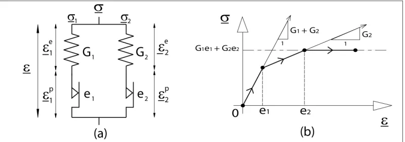
The one-dimensional two-element Venant model is composed of two elementary Saint-Venant models associated in parallel. It is characterized by the pairs ( , ), ( , ) such as < (Figure 2.a). Its behavior results from the summation of the stresses and , applied on each element. The total strain is the same for the two elements due to the parallel construction. If the strain of the model is less than the first threshold , the behavior is purely elastic and the two friction sliders are locked. If the strain becomes greater than or equal to , the first friction slider unlocks and the first spring locks, hence a loss of rigidity of value is recorded (Figure 2.b). Finally, if the strain of the model becomes greater than or equal to , the behavior becomes perfectly plastic.
Figure 2. Two-element Saint-Venant model (a) and its mechanical response (b).
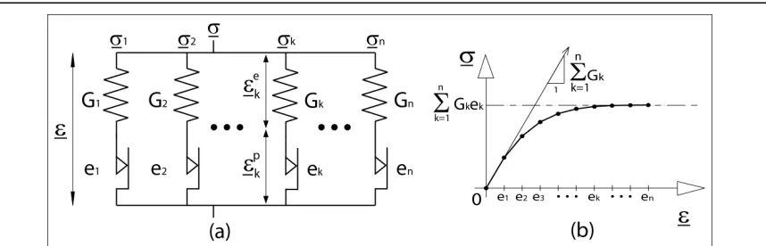
Figure 3. One-dimensional generalized Saint-Venant model (a) and its mechanical response (b).
Intrinsic Properties
The six essential intrinsic properties of the one-dimensional generalized Saint-Venant model are listed below (see Wack et al. (1992)):
1. The total strain in the model is the same for all the elements (Figure 3.a).
2. The first threshold strain tends toward zero, so that the model behavior is always irreversible (Figure 3.b).
3. At each reversal, all the friction sliders lock and the model gets back to its initial elastic modulus ∑ (Figure 4.a).
4. During a cyclic loading, the model observes Masing’s rule. This is illustrated Figure 4.a, where the unload curve CD is the image of the first load curve OC, by a homothety of ratio -2 and center H. Thus, point N', on the CD curve, is the image of point N on the OC curve. 5. During complex cyclic loading, the model can memorize events such as load reversals. This
is illustrated in Figure 4.a by the BAC reload and more particularly by the return to the first load behavior (OAC), after passing through point A.
6. Despite the irreversible behavior of the model, there is a neutral state that can be restored, after any mechanical loading, by a fundamental cycle. This property is illustrated by the cyclic loading OABACDE of Figure 4.a, which corresponds to an irreversible behavior, followed by a fundamental cycle EFO (Figure 4.b). This demagnetization-type cycle EFO consists of a cyclic loading of slowly decreasing strain amplitude through successive steps, until cancellation. The great property of a fundamental cycle is that a reload OG' after it shows a recovery of the initial behavior of first load (curve OG’ is the same as curve OC, as illustrated on Figure 4.a).
respectively. Then, the threshold strains are calculated as follows:
= (1)
= . with ∈ 1, (2)
To define the distribution of the spring elastic moduli , a generative function is adopted, such as:
= . ℎ !"
#". $ (3)
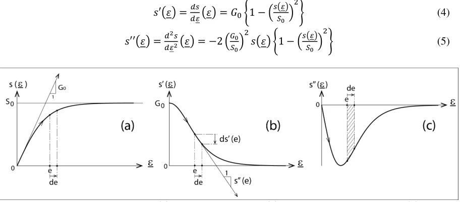
Where represents the initial elastic modulus at the origin and represents the yield limit. Figure 5 illustrates the shape of the generative function and its first and second derivatives, such as:
′ =&(&' = )1 − ' (#
" $ + (4)
′′ =&&(,', = −2 !"
#"$ )1 −
' (
#" $ + (5)
Figure 5. Generative function (a), first derivative ′ (b) and second derivative ′′ (c).
Let us consider the continuous one-dimensional generalized Saint-Venant model, which consists in replacing the discrete sequence of thresholds strains by a continuous sequence of elements indexed by a continuous threshold , varying from 0 to +∞. In this case, a section between and + is equivalent to an elementary Saint-Venant model with an elastic modulus − ′1 2 or − ′′1 2. . Thus, for a discrete sequence of thresholds , the spring elastic moduli are distributed such as:
= − ′′1 2. (6)
Figure 6. Distribution of spring elastic moduli .
One-Dimensional Generalized Saint-Venant Model with an Added Single Spring
The one-dimensional generalized Saint-Venant model can be completed with a single spring of elastic modulus 3 (Figure 7.a). This single spring then corresponds to an elementary Saint-Venant model characterized by an infinite threshold strain. In this case the quasi-reversible behavior, close to the origin and the load reversals, corresponds to an elastic modulus equal to the sum of all the spring elastic moduli, i.e. ∑ + 3 (Figure 7.b). The intersections between the straight line corresponding to the residual elastic modulus 3 and the y-axis, for > 0 and < 0, are the limiting thresholds ± ∑
respectively, as illustrated on Figure 7.b.
Figure 7. One-dimensional generalized Saint-Venant model completed with a single spring of elastic modulus 3 (a) and its mechanical response (b).
THREE-DIMENSIONAL GENERALIZED SAINT-VENANT MODEL
In the three-dimensional case, the friction sliders of the one-dimensional generalized Saint-Venant model are represented by Von Mises-like yield surfaces. During the loading, it is necessary to consider the relative positions of these surfaces with respect to each other and the loading history. The yield surfaces are described in Ilyushin’s five-dimensional deviatoric space (see Zyczkowski et al.
(1984)), in which they are represented by hyperspheres. The deviatoric part of symmetric second order tensors are described by five components vectors in an orthonormal frame of Ilyushin’s space (see Meggiolaro et al. (2016)).
In the remainder of this paragraph, the three-dimensional elementary Saint-Venant model and the three-dimensional generalized Saint-Venant are introduced. The yield surfaces and their movements are illustrated in the classical two-dimensional deviatoric plane.
Three-Dimensional Elementary Saint-Venant Model
(Figure 8.c). The elastic strain vector 88889 can then be deduced from the total strain vector 9 by:
88889 = 9− 88889 (7)
Figure 8. Elementary one-dimensional Saint-Venant model (a), three-dimensional stress-space (b) and strain-space (c) representations.
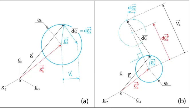
The movement of the yield surface in the strain space is driven by the flow rule. In this study, the normality flow rule, which implies that the plastic strain increment is orthogonal to the yield surface, is adopted. To define this motion, a vector :89 is introduced, such as:
:89 = 88889 + 88889 (8)
Where 88889 denotes a total strain increment during the loading, i.e. the transition from an instant to an instant + (Figure 9).
If the magnitude of vector :89 is less than or equal to the radius of the yield surface, i.e. ;:89 ; ≤ , the behavior is elastic and the center of the yield surface remains fixed (Figure 9.a):
If ;:89 ; ≤ then 88888889 = 089 ; 88888889 = 88889 and 88888889 = .88888889 (9)
On the contrary, if the magnitude of vector :89 is strictly greater than the radius of the yield surface, i.e. ;:89 ; > , then the behavior is elastic-plastic. In this case, the center of the yield surface
moves along an increment of plastic strain 88888889, collinear to vector :89. This flow is then orthogonal to the yield surface and complies with the flow rule normality (Figure 9.b):
If ;:89 ; > then 88888889 = =1 −;?889>
>;@ :89 ; 88888889 = 88889 − 88888889 and 88888889 = .88888889 (10)
Three-Dimensional Generalized Saint-Venant Model
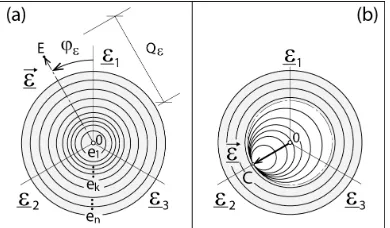
The three-dimensional generalized Saint-Venant model is characterized by a discrete sequence of threshold strains , defined by Equation 2, and by a distribution of the elastic moduli , defined by Equation 6. Figure 10 illustrates, in the two-dimensional deviatoric strain plane, the different yield surfaces corresponding to the discrete sequence of threshold strains. In the initial state, all the yield surfaces are centered at the origin of the deviatoric strain plane (Figure 10.a). During loading, all yield surfaces undergo the same total strain (Figure 10.b). The yield surfaces whose threshold has been reached slide (white yield surfaces on Figure 10.b) and the yield surfaces whose threshold has not been reached remain fixed (gray-colored yield surfaces, see Figure 10.b). In the two-dimensional deviatoric strain plane, a point such that E on Figure 10.a may be parameterized by a vector 9, which depends on two parameters: radius A( and phase B(. Similarly, in the two-dimensional deviatoric stress plane, the pair (AC,BC) is the radius and the phase respectively of a stress vector 9.
Figure 10. Illustration of yield surfaces in the two-dimensional deviatoric strain plane: initial state (a), state after a radial loading OC (b).
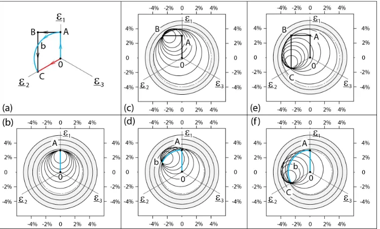
For each yield surface, the flow rule defined by Equation 9 and Equation 10 is adopted. That results in an independent movement of these surfaces, with respect to each other. This is illustrated in Figure 11, which shows simulation results in the two-dimensional deviatoric strain plane of three distinct loading paths that lead to the same point C: OC, OAbC, OABC (Figure 11.a). Figure 11.b shows the positions of the yield surfaces at the end of path OA. Figures 11.c and 11.d show the positions of the yield surfaces at points B and b respectively. Figures 10.b, 11.e and 11.f illustrate the final positions at point C of the yield surfaces, for each of the three loading paths. These three figures, which show relatively different configurations, illustrate a fundamental property of the model: it is highly sensitive to the loading history. This is confirmed by Figure 12.a, which gives distinct responses OC1, OAbC2, OABC3, in
Figure 11. Simulations in the deviatoric strain plane of three loading paths: OC, OAbC, OABC (a); yield surfaces position at the end of: path OA (b), path OAB (c), OAb (d), OABC (e), OAbC (f). Model
parameters: = 16 EF, = 286 HEF, 3= 1.6 EF, = 10, = 5 %.
Figure 12. Simulation results related to Figure 11; stress responses OC1, OAbC2, OCBC3, in the deviatoric
stress plane (a), corresponding to paths illustrated on Figure 11.a; responses in the rheological diagram (A(,AC) (b); deviatoric-plane phase difference between stress and strain (c).
Description of Cyclic Hardening Law Added to the Three-Dimensional Saint-Venant Model
To describe cyclic hardening or softening, the yield limit is replaced by the yield limit
1K , K 2 (Figure 13), where K and K are two cyclic hardening variables. The variable K corresponds
Figure 13. Illustration of the cyclic hardening law response in the case of a hardening material.
IMPLEMENTATION IN FEM CODE AND SIMULATION RESULTS
Tensorial Formulation of the Model
The constitutive equation is expressed with Cauchy stress tensor M, Almansi strain tensor Nand Lamé coefficients (O,P). The model is written in Jaumann’s co-rotational reference frame. This model can therefore take into account finite strains and finite rotations. The constitutive equation is in the form:
M = O + RQ$ . ST1N2. U + ∑ . NVW+
3. N (11)
Implementation in FEM Code, Model Parameters and Identification
The three-dimensional Saint-Venant model has been implemented in FEM code Abaqus (Abaqus 6.13 (2013)), using a user-subroutine UMAT. This subroutine contains 2 numerical parameters and , 4 material parameters for the pure hysteresis part , X (Poisson’s ratio), and 3, and 3 material parameters for the cyclic hardening law L , F and F .
The four parameters of the pure hysteresis part are identifiable with a reduced number of uniaxial tensile tests (5 tests, for repeatability, are sufficient). The three cyclic hardening parameters can be identified with alternating torsion tests using the cyclic hardening and cyclic consolidation curves.
Validation of the Three-Dimensional Generalized Saint-Venant Model
The three-dimensional generalized Saint-Venant model has been validated using confrontations with different experimental results. In this section, the pure hysteresis behavior without cyclic hardening is considered. An hourglass-type path in tension-torsion, performed by Aubin (2001) is considered (Figure 14.a). The four materials parameters have been identified with a monotonic uniaxial tensile curve. The simulation results, in bold lines Figure 14, reproduce in a very satisfactory manner the experimental data in dotted lines, either for the stress response (Figure 14.b), the response in the tensile direction (Figure 14.c) and the response in the shear direction (Figure 14.d).
tests. A three-parameter cyclic hardening law is also proposed to capture the behavior evolution between the first load and the stabilized cycle. The model thus developed provides accurate results in the case of non-proportional loadings. Experimental tests are in progress and may complete this work, on the one hand to confirm the results obtained in pure hysteresis and on the other hand to validate the proposed cyclic hardening law.
ACKNOWLEDGMENT
The support from GE Renewable Energies, Hydro’Like Chair and Fondation Grenoble INP is greatly appreciated.
NOMENCLATURE
\ or ] : Symmetric second order tensor
\ or ] : Deviatoric part of a symmetric second order tensor
F9 or ^9 : Vector (can be a symmetric second order tensor written in vector form) F9 or ^9 : Deviatoric part of a second order tensor written in vector form
F or ^ : Scalar
F or ^ : Scalar where the underlining recalls its deviatoric nature
NW, N_ : Elastic part and plastic part of Almansi strain tensor respectively
U : Second order identity tensor
REFERENCES
Abaqus 6.13, (2013). “Abaqus documentation,” Dassault Systèmes Simulia Corp., Providence, RI, USA. Aubin, V., (2001). “Plasticité cyclique d’un acier inoxydable austéno-ferritique sous chargement biaxial
non-proportionnel,” Ph.D. Thesis, France.
Brown, A.A., Casey, J., Nikkel, D.J., (2003). “Experiments conducted in the context of the strain-space formulation of plasticity,” Int. J. Plasticity, 19 1965-2005.
Guélin, P. (1980). “Remarques sur l’hystérésis mécanique,” J. Mécanique Théorique et Appliquée,
France, 19(2) 217-247.
Heiduschke, K., (1995). “The logarithmic strain space description,” Int. J. Solids Structures, 32 1047-1062.
Lee, J.H., (1995). “Advantages of strain-space formulation in computational plasticity,” Computers and
Structures, 54 515-520.
Meggiolaro, M.A., Pinho de Castro, J.T., Wu, H., (2016). “A general class of non-linear kinematic models to predict mean stress relaxation and multiaxial ratcheting in fatigue problems – Part I: Ilyushin spaces,” Int. J. Fatigue, 82 158-166.
Naghdi, P.M., Trapp, J.A., (1975). “The significance of formulating plasticity theory with reference to loading surfaces in strain space,” Int. J. Engng. Sci., 13 785-797.
Persoz, B. (1960). “Introduction à l’étude de la rhéologie,” Dunod, France.
Wack, B., Tourabi, A., (1992). “Some remarks on macroscopic observations and related microscopic phenomena of the mechanical behavior of metallic materials,” Arch. Mech., 44 621-662.


![Diethyl 2,6 dimethyl 4 [5 (4 methylphenyl) 1H pyrazol 4 yl] 1,4 dihydropyridine 3,5 dicarboxylate](data:image/gif;base64,R0lGODlhAQABAIAAAP///wAAACH5BAEAAAAALAAAAAABAAEAAAICRAEAOw==)