Asynchronous Hierarchical Parallel Evolutionary Algorithm-Based Framework for Water Distribution Systems Analysis.

(1)

ABSTRACT

KUMAR, JITENDRA. Asynchronous Hierarchical Parallel Evolutionary Algorithm-Based Framework for Water Distribution Systems Analysis. (Under the direction of G. Mahinthakumar and S. Ranji Ranjithan.)

Water distribution systems (WDSs) are vulnerable to accidental and intentional contamination that can have serious effect on the public health. Accurate characterization of the contaminant source is usually the first step in designing a response strategy for control and containment of the contaminant during an event. Contaminants can spread quickly in the network due to complex hydraulic conditions requiring a procedure for near real-time identification of the source characteristics and design of response strategy. Limitations associated with the quality and quantity of network monitoring data, unknown nature of the contaminant and its interaction with other chemicals in the water, complexity of the network, and inherent uncertainties make contaminant source characterization a difficult and challenging problem to solve. Solution of source characterization problems requires iterative simulations of flow and transport, which are highly computing intensive posing a computational challenge for near real-time solution of the problem.

(2)

characterization under the conditions of such uncertainties and noise in the system are examined. These methods are applied and tested for an array of contamination scenarios in two different example networks. To enable a near real-time solution, a massively parallel computational framework is developed for modern shared/distributed memory architecture-based parallel computers. This includes the development of a new Asynchronous Hierarchical Parallel Evolutionary Algorithm (AHPEA) to solve complex large-scale global optimization problems. Performance and robustness of AHPEA algorithm is tested using a suite of benchmark function optimization problems and its application to address water distribution contaminant threat management problems is demonstrated. A WDS simulation model and the optimization methodologies are fully integrated into the computational framework for real-time analysis of the system. The computational framework is tested for parallel performance and scaling on different state-of-the-art parallel computers.

(3)

Asynchronous Hierarchical Parallel Evolutionary Algorithm-Based Framework for Water Distribution Systems Analysis

by Jitendra Kumar

A dissertation submitted to the Graduate Faculty of North Carolina State University

in partial fulfillment of the requirements for the Degree of

Doctor of Philosophy

Civil Engineering

Raleigh, North Carolina 2010

APPROVED BY:

--- --- Dr. E. Downey Brill, Jr. Dr. Jeff A. Joines

(4)

ii

DEDICATION

Dedicated to

my parents, sisters and brother

(5)

iii

BIOGRAPHY

(6)

iv

ACKNOWLEDGEMENTS

I wish to express my sincere gratitude to my advisors Dr. G. Mahinthakumar and Dr. Ranji Ranjithan for their guidance, support and encouragement throughout this work. It was a privilege to work with and learn from two great teachers, the skills for problem solving and critical thinking. In the weekly breakfast meetings with Dr. Ranjithan over the last few years, I have learnt a lot more than just research, which would help me a long way in my career. I would like to thank Dr. Downey Brill for his constant support and encouragement. He is undoubtedly the best teacher I ever had. I would also like to thank my committee member Dr. Jeff Joines for his invaluable suggestions and time. I have had an opportunity to interact, learn and share ideas with many other professors in the department and I am very thankful to all of them.

I would also like to acknowledge my officemates and colleagues for the thoughtful discussions, research collaborations, feedback and support. Special thanks to Sarat Sreepathi and Li Liu for their support and collaboration as a team on NSF DDDAS project. I would like to thank the wonderful group of friends in Mann 431 and the department including, Naresh Devineni, Vamsi Sripathi, Jason Simon, Danielle Touma, Brandon Graver, Silesh Amujuri, Ali Mehran and many others for the great fun filled days and amazing „Fridays‟ at NC State. I also want to thank my friends Salil Wadhavkar and Pradeep Sharma for their help and support.

(7)

v

LIST OF FIGURES

(12)

x

Figure 2.14 Potential locations for contamination source for Scenario 10 ... 29

Figure 2.15 Potential locations for contamination source for Scenario 11 ... 30

Figure 2.16 Layout of the Micropolis water distribution network ... 31

Figure 2.17 Contamination injection pattern for the true source in Scenarios 12 and 13... 32

Figure 2.18 Potential source locations identified in the ten random trials for Scenario 12 .... 33

Figure 2.19 source locations identified in the ten random trials for Scenario 13 ... 34

Figure 3.1 Evolutionary algorithm for generating alternatives ... 45

Figure 3.2 Network 1 layout and contamination scenario ... 48

Figure 3.3 Micropolis water distribution network ... 49

Figure 3.4 Injection loading profiles for four solutions of scenario 1 ... 55

Figure 3.5 Convergence of the ES-based search for subpopulation ... 56

Figure 3.6 Injection profiles for two solutions of Scenario 2 ... 57

Figure 3.7 Injection profiles for four solutions of Scenario 3 ... 59

Figure 3.8 Injection profiles for seven solutions of Scenario 4 ... 61

Figure 3.9 Average prediction error for the best-fit solutions for each scenario over 50 random trials ... 62

(13)

xi

Figure 3.11 Average (horizontal bar) and one-standard deviation (vertical bar) of the number

of solutions obtained for each scenario over 50 random trials ... 64

Figure 3.12 Potential contamination source locations for Scenarios 1-4... 65

Figure 3.13 Potential sorce locations for Scenario 5 ... 66

Figure 3.14 Potential source locations for Scenario 6 ... 67

Figure 4.1 Observed chlorine concentrations at a sensor under 1st/2nd order reaction conditions ... 76

Figure 4.2 Network 1 water distribution system ... 80

Figure 4.3 Micropolis water distribution system ... 80

Figure 4.4 Arsenic injection pattern for a typical solution for Scenario 1 ... 83

Figure 4.10 Asenic injection pattern for a typical solution for Scenario 7 ... 90

(14)

xii

Figure 5.1 Examples of hierarchical population topologies ... 102

Figure 5.2 Base serial genetic algorithm ... 104

Figure 5.4 Asynchronous Hierarchical Parallel Evolutionary Algorithm (AHPEA) ... 106

Figure 5.5 Typical convergence of each population in the three-population AHPEA (AHPEA-3) for the 100-dimensional (D=100) Shifted Ackley's function ... 113

Figure 5.6 Typical convergence of each population in the ten-population AHPEA (AHPEA-10) for the 100-dimension Shifted Ackley's function ... 114

Figure 6.1 Population to processor mapping in AHPEA for a 10 population EA ... 125

Figure 6.2 File I/O modes in the AHPEA framework ... 126

Figure 6.3 Migration of individuals using MPI-2 one sided communication ... 128

Figure 6.4 Sharing of centroid information among the populations ... 129

Figure 6.5 Simulation-optimization model integration into AHPEA using MPI-2 dynamic process creations ... 131

Figure 6.6 Scaling of AHPEA for different problem sizes solved on the Cygnus system at NCSU)... 133

(15)

xiii

Figure 6.9 AHPEA-pEPANET scaling for increasing population size when solved on Cygnus

system at NCSU ... 137

Figure 7.1 Simulation-optimization framework ... 143

Figure 7.2 Evolutionary algorithm based optimization model ... 146

Figure 7.3 File based coupling of simulation-optimization models ... 147

Figure 7.4 MPI-2 dynamic process based simulation-optimization coupling ... 150

Figure 7.5 Micropolis water distribution network ... 152

Figure 7.6 Study contamination scenario and results ... 153

Figure 7.7 Scaling study of file based and MPI-2 based versions ... 155

Figure 7.8 Percentage of time spent in I/O operations for the two versions (Abe, NCSA TeraGrid)... 156

(16)

xiv

LIST OF TABLES

Table 2.1 Details of the scenarios analyzed ... 16

Table 2.2 Algorithmic parameter settings for the NCES algorithm ... 17

Table 2.3 The source location and injection start time of the non-unique solutions obtained for a typical trial for Scenarios 1-4 ... 19

Table 2.4 The average prediction error (number of mishits) for non-unique sources located at nodes 10, 12, and 86 ... 25

Table 2.5 The set of solutions obtained for a typical trial for Scenario 10 ... 29

Table 2.6 The set of solutions obtained for a typical trial for Scenario 11 ... 30

Table 3.1 The set of solutions from a representative trial for Scenario 1 ... 53

Table 3.5 Potential locations for alternative solutions for different scenarios ... 64

Table 4.1 Scenarios analyzed for the two example networks ... 82

Table 5.1 Results obtained using serial algorithm for the 100 dimensional (D=100) versions of the test problems. The results are based on 25 random trials. ... 110

(17)

xv

(18)

1

CHAPTER 1.

Introduction

Water distribution systems (WDS) consist of large network of pipes and utilities to enable the supply of fresh drinking water supply to every household. Because of the large spatial extent of these systems, it is not possible to ensure the physical security of the system. WDS are highly interconnected in nature with numerous possible access points in the system making it vulnerable to accidental or intentional contamination. WDS networks are designed purposely for a high degree of redundancy for mixing at the nodes of the network so that the disinfectant (i.e., free chlorine) reaches all parts of the network. Thus, any external contaminant can spread quickly through mixing and transport and might be consumed by consumers, possibly leading to severe public health emergency. During a contamination event, large number of consumers can potentially be affected unless control measures are taken immediately. Accurate knowledge of the possible contamination source characteristics is needed for the design of a control and response strategy in the event of a contamination.

(19)

2

system to normal in shortest possible time, a near real-time solution of the problem is required.

The objective of this research is to develop new algorithms, methodologies and computational tools to address the contaminant source identification in a WDS for a wide range of possible contamination scenarios discussed above.

Source characterization problem can be posed as inverse problem and can be solved using a simulation-optimization approach. Optimization model is used to identify the characteristics of the contaminant source and simulation model is used to predict the contaminant concentration distribution in the network for a given network configuration and demand condition. Optimization problem for source identification involve several discrete and continuous variables. Also, non-uniqueness in the solution is a major issue with more than one set of source characteristics possible to match the observations at the sensors equally well. Determining a single solution might lead to misleading assessment of the contamination event. Thus, the optimization problem needs to be solved not just for a single best solution but all possible solutions which fit the observations. An evolutionary algorithm based simulation-optimization methodology has been developed in this research for the identification of contaminant source characteristics in WDS. The multiple-population optimization algorithm employs a method for generating alternative solutions to address the issue of non-uniqueness in source characterization problems.

The source identification problem was studied using the data from various kinds of sensors providing continuous and accurate observations to filtered threshold based binary signals. Effect of quality and quantity of water quality sensor data on the accuracy and non-uniqueness of source characterization problem was studied in detail. Effect of observation data noise and uncertainties were also studied in detail.

(20)

3

methodology was developed to use routinely recorded chlorine measurements as surrogate to detect the presence of a reactive contaminant in the system and to identify the source characteristics. The issues of uncertainty about the reaction kinetics and parameters and noise in the observation data were studied.

To minimize the impact of a contamination and to develop a response strategy, real time solution of the source identification is needed. However, simulation of a water distribution system is computationally intensive requiring enormous computation for the solution of the inverse problem. A new parallel evolutionary algorithm was developed in this research to enable the solution of large scale optimization problems in near real-time. An asynchronous hierarchical parallel evolutionary algorithm was developed to address the class of large scale global optimization problems in general and was successfully applied for the near real-time solution of WDS source identification problem.

All the algorithms and methods were incorporated into an integrated parallel simulation-optimization framework and were tested on a range of parallel platforms from small clusters to massively parallel supercomputers. An extensive series of parallel performance studies were carried out to optimize the computational performance of the framework.

1.1

Organization of the dissertation

The research conducted in this study has been organized in the dissertation as follow. Chapter 2 describes the development of contaminant source identification method for WDS using imperfect binary sensors. Analysis of the effect of quality and quantity of water quality observation data on accuracy and non-uniqueness of source identification problem has also been reported.

(21)

4

Chapter 4 describes the methodology for source identification in WDS involving reactive contaminants.

Chapter 5 presents a new Asynchronous Hierarchical Parallel Evolutionary Algorithm (AHPEA) framework for large scale global optimization problems.

Chapter 6 describes the design of massively parallel computational framework for the AHPEA and results of the parallel performance analysis conducted on several different parallel platforms.

Chapter 7 describes the development of a computational cyberinfrastructure for contaminant threat management in WDS. Computational framework for coupling of simulation and optimization model has been presented and computational performance results have been reported.

(22)

5

CHAPTER 2.

Contaminant source characterization in water

distribution systems using filtered sensor data

2.1

Introduction

Water distribution systems are vital for supplying safe drinking water to the public, and they are vulnerable to contamination that can be introduced into the system either deliberately or accidentally. The fate and transport of a contaminant and the extent of the contaminant spread through the network depend on the characteristics of the network topology and the resulting hydraulic conditions of the network.

Networks of sensors can be used as an early warning system to detect sudden deterioration in water quality. They are meant to supplement conventional water quality monitoring by quickly providing timely information on unusual threats to a water supply system. The goal of an early warning system is to reliably identify a contamination event in the distribution systems in time to allow an effective targeted response that reduces or avoids entirely the adverse effects of contamination on the system. The contaminant source characterization (i.e., identifying the contaminant source location and injection pattern) problem has been approached as an inverse problem by many researchers (e.g., Waanders et al. 2003; Laird et al. 2005, 2006; Guan et al. 2006). These approaches attempt to reconstruct a contamination injection event by matching the estimated contaminant concentration profiles with the observations at contaminant sensor locations.

(23)

6

defined here to be determined by the detection threshold level; i.e., a more sensitive (therefore more expensive) binary sensor will have a lower detection threshold. A contamination event may even go undetected if the installed sensors have a low sensitivity. Thus, in addition to lowering of information quality due to inherent data filtering in a binary sensor, the sensitivity of the binary sensor also affects the quality of the information used to estimate the source characteristics. Such sensor data quality issues along with errors and uncertainties in model and data associated with a water distribution system results in potential ambiguities in the predicted contaminant source characteristics. One implication is that there may be non-unique solutions to the inverse problem such that a set of different source characteristics match the observations at the sensors. This limits the ability to precisely identify the true source location and the contaminant injection pattern.

The work presented in this paper describes a methodology for characterizing the contaminant source in a particular event using detection signals from a set of binary sensors. This work also includes an investigation of the effect of the quality (i.e., sensitivity of the sensors) and quantity (i.e., number of sensors in the network) of the sensor data on the accuracy in identifying the source characteristics and on resolving the degree of non-uniqueness. The methodology is applied and tested on realistic water distribution networks to assess its applicability and robustness.

2.2

Data filtering effects in binary sensors

(24)

7

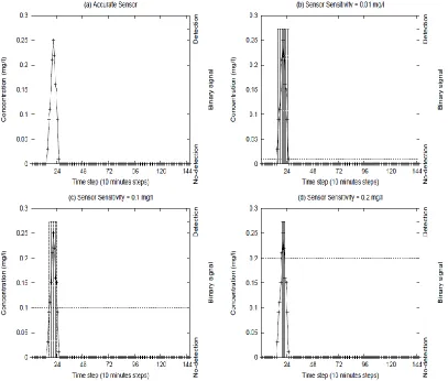
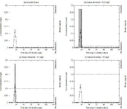
Figure 2.2.a shows the continuous concentration profile with relatively low concentration values, and Figure 2.2.b-Figure 2.2.d show the filtered binary signals for sensors with detection threshold of 0.01 mg/l, 0.1 mg/l, and 0.2 mg/l, respectively. Considering Figure 2.1.b and Figure 2.2.b, there is no discernible difference when comparing the binary signal profiles for the 0.01 mg/l threshold even though the real concentration profiles are different and may have resulted from different contaminant injection patterns. Such effects of data filtering at binary sensors can potentially contribute to non-uniqueness and lack of precision in the source characteristics being identified.

Figure 2.1 Effect of sensor threshold on the filtering of data to produce a binary signal:

(25)

8

Figure 2.2 Effect of sensor threshold on the filtering of data to produce a binary signal:

Example 2

2.3

Characterization of the contaminant source using binary sensor data

(26)

9

(i.e., the location and injection pattern), the binary sensor signals are simulated and compared to the observations. The prediction error is then used as a measure of goodness of fit to direct the search for a set of source characteristics that best fits the observations. The resulting search problem is solved using a coupled simulation-optimization approach.

The following characteristics of the contaminant source are decision variables for the optimization problem:

(a) Location (L) of the contaminant source in the network. Location of the source is assumed to be at one or more of the nodes in the WDS network.

(b) Start time of the contaminant injection into the system (T0). Start time is measured

as the time elapsed from the start time of the simulation.

(c) The pattern of contaminant injection (C0) into the system measured in terms of

milligrams of contaminant injected per minute into the system. Injection rate is assumed to be constant during each water quality time step of the simulation. No assumptions are made regarding the magnitude, pattern or duration of the contaminant injection.

The optimization model for this inverse problem is defined below (Equations 1-3) assuming that the contamination scenario involves only a single source; however, it could be extended to scenarios involving simultaneous contamination at multiple sources.

, ,

1 1

, 0 0

,

, 0 0

, ,

,

(1)

0, ( , , )

( 2 ) 1, ( , , )

0, (3) 1, S S N T s a

i t i t

i t

s

i t th

s

i t _s

i t th

a i t th a

i t _a

i t th

M in im ize E B S B S

if C L T C C

su b ject to B S

if C L T C C

if C C

w h ere B S

(27)

10

The objective function (Equation 1) is a measurement of error represented as the total number of mishits at the sensors. A simulated expected signal for the given values of L, T0,

and C0, will be considered a mishit if it does not match the actual signal. Specifically, there is

a mishit when there is a simulated detection signal when the actual signal was of no-detection or vice versa. The optimization problem is to obtain the values of L, T0, and C0 that minimize

the total number of mishits between the simulated and actual sensor signals. Equation 2 filters the simulated concentration levels for a given set of source characteristics at the sensors into detection/no-detection binary signals depending on the sensitivity of the sensor for the particular contaminant. s_,

i t

B S and a_, i t

B S are respectively, the simulated binary signal and the actual binary signal for given source characteristics at sensor i at any time t; Ns is the

number of sensors in the network; TS is the total time for which contaminant mixing and

transport in the network is being simulated. The simulated concentrations of the contaminant are given by C_{i t}s_, ( ,L T C₀, ₀) for a given solution as a function of location (L), time of measurement (t), start time of the contamination injection (T0), and the contaminant injection

pattern (C0), respectively.

Cth is a constant defining the threshold concentration level for determining detection and

generating a binary signal by the sensors. The constants a_, i t

C are the actual measured concentrations of the contaminant being monitored.

2.4

Methodology

(28)

11

and be able to identify the set of potential source characteristics that provide equally good fit to the given observations. The niched co-evolution strategies (NCES) search procedure (Zechman and Ranjithan, 2004, 2007) was used to solve the above model. Also, given the possibility of error in modeling of the physical distribution network, it is also important to identify near optimal model solutions that might be the solution to the real problem. The NCES procedure also provides this capability.

NCES conducts a global search using evolution strategies (ES), a generalized heuristic optimization approach. A ES works in a continuous space and has the capability to self adapt its major algorithmic parameters such as selection and mutation. ES starts with a randomly initialized population of μ individuals. A probabilistic mutation operator is applied to produce λ new solutions each generation. The next set of individuals is selected from either a combined set of parent and offspring solutions (denoted as (μ + λ) selection) or from the set of offspring alone (denoted as (μ, λ) selection).

(29)

12

selection step. However, the distance measure can easily be extended to include time and contaminant injection pattern also.

While one subpopulation focuses its search on finding the optimal solution based on the prediction error (E in Eqn. 1), the other subpopulations search for alternatives based on the current best prediction error value as well as the degree of difference among the alternative solutions. In the results presented in this paper, every solution that is within one miss-hit from the best prediction error value (i.e., E = 1) is considered as a viable alternative solution.

NCES was applied and tested on two water distribution networks to study: 1) the effect of the sensitivity of binary sensors (quality of data) on the accuracy and non-uniqueness of the solutions to such source identification problems; 2) the effect of the quantity of available data (i.e., number of installed sensors) on the solutions to source identification problems; and 3) the robustness of the method when applied to a set of different contamination scenarios and networks.

2.5

Illustrative case studies

2.5.1 Networks analyzed

(30)

13

(a) Network (b) Injection pattern

Figure 2.3 Layout of the Network 1 water distribution network

(31)

14

Figure 2.4 Layout of the Micropolis water distribution network

2.5.2 Scenarios analyzed

Network 1 was used to construct several hypothetical contamination scenarios (Table 2.1) designed to investigate various aspects of the source characterization problem that is to be solved based on observations from a set of threshold-based binary sensors.

Scenario 1 was designed to serve as a benchmark for an ideal scenario in which

continuous and accurate concentration measurements of the contaminants are assumed to be available. The sum of the squared error between the actual and simulated concentrations at the sensors was used as the metric to be minimized in the optimization problem. Equation 4 represents the mathematical formulation of the objective function for this scenario.

2

2 2

, 0 0 ,

1 1

( , , ) / m in .

S s

N T

s a

i t i t

i t

M in im ize E C L T C C m g

(32)

15

In Scenarios 2, 3 and 4, the sensitivity of the binary sensor was set at 0.2 mg/l, 0.1 mg/l

(33)

16

Table 2.1 Details of the scenarios analyzed

Scenario True source location Node No. (Network)

Sensor type Sensor sensitivity

No. of sensors

Contaminant injection profile

1 12 (Network 1) Ideal - 6 Continuous (1 hr.)

2 12 (Network 1) Binary 0.2 mg/l 6 Continuous (1 hr.)

8 12 (Network 1) Binary 0.1 mg/l 6 Intermittent

9 12 (Network 1) Binary 0.1 mg/l 6 Intermittent

12 787 (Micropolis) Binary 0.1 mg/l 5 Continuous (1 hr.) 13 653 (Micropolis) Binary 0.1 mg/l 5 Continuous (1 hr.)

(34)

17

In all scenarios, the search was conducted to identify up to five alternative potential solutions by including five subpopulations in NCES. Subpopulation 1 was designed to search for the solution with the minimum number of mishits, while the other subpopulations were set to search for alternative solutions that are maximally different from each other and have no more than one mishit more compared to the lowest number of mishits (i.e., the minimum objective function value for subpopulation 1). The NCES algorithmic parameters used in this study are shown in Table 2.2.

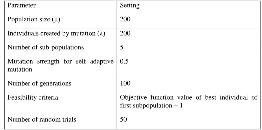
Table 2.2 Algorithmic parameter settings for the NCES algorithm

Parameter Setting

Population size (μ) 200

Individuals created by mutation (λ) 200 Number of sub-populations 5 Mutation strength for self adaptive mutation

0.5

Number of generations 100

Feasibility criteria Objective function value of best individual of first subpopulation + 1

Number of random trials 50

2.6

Results

(35)

18

identified; and 4) locations of all the feasible non-unique solutions identified in the 50 random trials.

2.6.1 Ideal water quality sensor measurements (based on Scenario 1)

(36)

19

Figure 2.5 Contamination injection profiles for a typical solution for Scenario 1 and the true

source

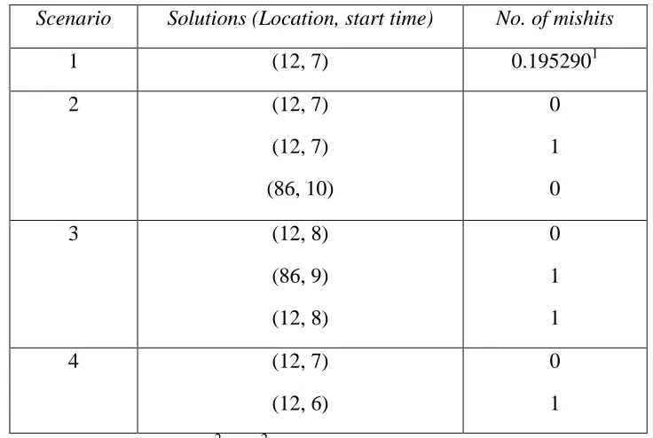
Table 2.3 The source location and injection start time of the non-unique solutions obtained for a typical trial for Scenarios 1-4

Scenario Solutions (Location, start time) No. of mishits

1 (12, 7) 0.1952901

2 (12, 7)

(12, 7) (86, 10)

0 1 0

3 (12, 8)

(86, 9) (12, 8)

0 1 1

4 (12, 7)

(12, 6)

0 1

1

(37)

20

2.6.2 Effect of quality of data (based on Scenarios 2, 3, and 4)

Scenarios 2-4 were run with different values of sensor sensitivity to study the effect of data quality (due to different degrees of data filtering in the binary sensor) on level of non-uniqueness. In each case, 50 trials were run to assess the number of alternative solutions and the relative locations of the source nodes associated with the non-unique solutions.

2.6.2.1Scenario 2: Sensor sensitivity = 0.2 mg/l

(38)

21

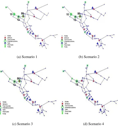
(a) Scenario 1 (b) Scenario 2

(c) Scenario 3 (d) Scenario 4

Figure 2.6 Potential contamination source locations identified by the set of non-unique

solutions for Scenario 1-4

2.6.2.2Scenario 3: Sensor sensitivity = 0.1 mg/l

(39)

22

matched the observation data with a single mishit. Third solution that was identified at the true source location matched the observation data with a single mishit. A solution perfectly matching the observed data was always identified among the set of feasible solutions obtained for each of the 50 trials. Locations of these non-unique solutions are shown in Figure 2.1.c. Based on the 50 trials, on average 2.12 alternative solutions (with a standard deviation of 0.961) were identified with average prediction error of 0.887 mishits and standard deviation 0.238 mishits.

2.6.2.3Scenario 4: Sensor sensitivity = 0.01 mg/l

(40)

23

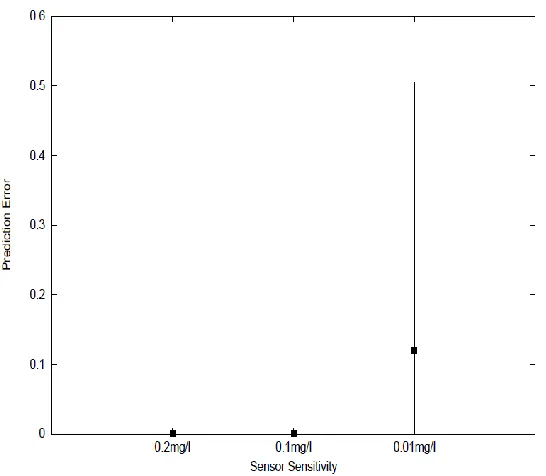
Figure 2.7 For Scenarios 2, 3 and 4, the average (horizontal bar) and one-standard deviation (vertical bar) of prediction error of the best solutions obtained for the 50 trials

(41)

24

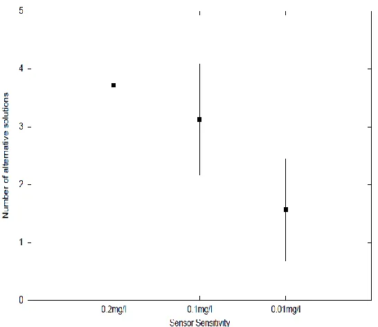
Figure 2.9 For Scenarios 2, 3 and 4, the average (horizontal bar) and one-standard deviation (vertical bar) of the number of non-unique solutions obtained for the 50 trials

(42)

25

Table 2.4 The average prediction error (number of mishits) for non-unique sources located at

nodes 10, 12, and 86

Location Scenario 2 Scenario 3 Scenario 4

Node 10 1.0 N/A1 N/A1

Node12 0.671053 0.523438 0.347222

Node 86 0.55 1.0 N/A1

1 no feasible solution with no more than one mishit was found

2.6.3 Effect of quantity of data (based on Scenarios 5, 6, and 7)

2.6.3.1Scenario 5, 6, 7

The amount of data available for characterizing the source has a significant impact on the source identification problem, which was studied using several scenarios with different numbers of water quality sensors. Scenarios 5, 6, and 7 include 6, 3, and 1 binary sensor, respectively, in the network, and the sensitivity of the sensors was assumed to be 0.1 mg/l. It was observed that as the amount of data decreases with the decreasing number of sensors, the number of alternative solutions that fit the observations (i.e., non-uniqueness) increases. Figure 2.10, Figure 2.11 and Figure 2.12 show the alternative source locations in the network for 6, 3 and 1 sensor scenarios, respectively, and the number of locations where alternative sources were found was 2, 13, and 13 for Scenario 5, 6, and 7, respectively.

(43)

26

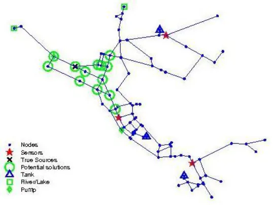
Figure 2.10 Potential source locations identified for the 6-sensor case (Scenario 5)

(44)

27

Figure 2.12 Potential source locations identified for the 1-sensor case (Scenario 7)

2.6.4 Testing under different contamination scenarios (based on Scenarios 8, 9,

10, and 11)

2.6.4.1Scenario 8, 9: Intermittent contaminant injection

(45)

28

(a) (b)

Figure 2.13 Intermittent contaminant injection pattern used in Scenario 8 (a) and Scenario 9 (b)

For both the scenarios, feasible solutions were identified at the true source location (Node 12) and an adjacent node (Node 86). For Scenario 8, the best solution in the first subpopulation was identified with an average error of 1.0 mishit and standard deviation of 1.069 mishits, and on average 1.24 (with a standard deviation of 1.238) alternative solutions were identified. The average prediction error for alternative solutions was found to be 1.398 mishits with a standard deviation of 1.299 mishits. Similarly, for Scenario 9, the average error of the best solution was 0.64 mishit (standard deviation 0.942 mishit), and on average 0.86 (with a standard deviation of 0.989) alternative solutions were identified with an average prediction error of 0.945 mishit (and standard deviation of 1.1612 mishits).

2.6.4.2Scenario 10, 11: Different source locations

To test the ability of the source identification method to identify a source existing at different locations in the network, in scenarios 10 and 11 the source location was placed at Node 20 and Node 54, respectively (Figure 2.14, Figure 2.15). The contaminant injection pattern was the same as in Scenarios 1-7. Six binary sensors with a sensitivity of 0.1 mg/l were included.

(46)

29

solution was identified by the first subpopulation during each of the 50 trials. On average 3.84 (with a standard deviation of 0.370) alternative solutions were identified. The average error for the alternative solutions was 0.83 mishit (with a standard deviation of 0.222 mishit).

Table 2.5 The set of solutions obtained for a typical trial for Scenario 10

Solution Location Start time No. of mishits

1 18 11 0

2 17 12 1

3 13 11 1

4 85 11 1

5 20 8 1

Figure 2.14 Potential locations for contamination source for Scenario 10

(47)

30

all 50 random trials. In all cases, four alternative solutions were identified with a mean error of 0.925 mishit (with a standard deviation of 0.1450 mishit).

Table 2.6 The set of solutions obtained for a typical trial for Scenario 11

Solution Location Start time No. of miss-hits

1 54 7 0

2 18 2 1

3 17 2 1

4 17 5 1

5 17 1 1

Figure 2.15 Potential locations for contamination source for Scenario 11

2.6.5 Testing for a different network (based on Scenarios 12 and 13)

(48)

31

here are two scenarios (12 and 13) with the contamination source located at Node 787 and Node 653, respectively. In both scenarios the contamination source was assumed to be active for one hour starting at 12.00am (i.e., at time step 1) with a injection pattern as shown in Figure 17. For each scenario, the source characterization method was applied with 50 subpopulations to search for a maximum of 50 alternative solutions. Alternative solutions within a single mishit from the best solution were accepted as a feasible solution to the problem. The statistics of the solutions obtained for ten random trials are reported for each scenario.

(49)

32

Figure 2.17 Contamination injection pattern for the true source in Scenarios 12 and 13

2.6.5.1Scenario 12

(50)

33

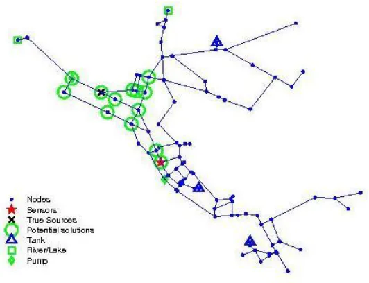
Figure 2.18 Potential source locations identified in the ten random trials for Scenario 12

2.6.5.2Scenario 13

(51)

34

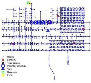
Figure 2.19 source locations identified in the ten random trials for Scenario 13

Results for Scenarios 12 and 13 demonstrate that the methodology described in this paper is able to solve the contaminant source characterization problem for the Micropolis example, which represents a medium-sized network. Besides consistently identifying the true source characteristics, it was also able to identify a set of non-unique solutions that is expected to fit the limited observations. Although the prediction error is relatively higher, the set of alternative source locations is able to pinpoint the potential source location to an area around the true source location.

2.7

Conclusions

(52)

35

monitored using a set of sensors that report a binary signal based on the presence of contamination. The source characteristics were reconstructed using these binary signals.

(53)

36

References

Brumbelow, K., Torres, J., Guikema, S., Bristow, E., and Kanta, L. (2007). “Virtual Cities for Water Distribution and Infrastructure System Research.” World Environmental and Water Resources Congress2007, Tampa, FL.

Dandy, G. C., Simpson, A. R., and Murphy, L. J. (1996). “An Improved Genetic Algorithm for Pipe Network Optimization.” Water Resources Research, 32(2), 449-458.

Holland, J. H. (1975). Adaptation in Natural and Artificial Systems: An Introductory Analysis with Applications to Biology, Control, and Artificial Intelligence. MIT Press, Cambridge, MA.

ILSI (1999). “Early warning monitoring to detect hazardous events in water supplies.” International Life Sciences Institute-Risk Science Institute.

Kumar, J., Zechman, E. M., Brill, E. D., Mahinthakumar, G., Ranjithan, S., and Uber, J. (2007). “Evaluation of Non-Uniqueness in Contaminant Source Characterization Based on Sensors with Event Detection Methods.” World Environmental and Water Resources Congress 2007, Tampa, FL.

Laird, Carl D., Biegler, Lorenz T., van Boleman Waanders, Bart G., Barlett, and Roscoe A. (2005). “Contamination source determination for water networks.” Journal of Water Resources Planning and Management, Vol. 131(2), 125-134.

Laird, Carl D., Biegler, Lorenz T., van Boleman Waanders, Bart G. (2006). “A Mixed-integer approach for obtaining unique solutions in source inversion of drinking water networks.” Journal of Water Resources Planning and Management, 132(4), 242-251.

(54)

37

McKenna, Sean. A., Hart, David., Klise, Katherine., Cruz, Victoria., and Wilson, Mark. (2007). “Event detection from water quality time series.” World Water and Environmental Congress 2007, Tampa, FL.

USEPA (2005), “Technologies and techniques for early warning systems to monitor and evaluate drinking water quality: A state-of-art review.”

Savic, D. A. and Walters, G. A. (1997). “Genetic Algorithms for Least-Cost Design of Water Distribution Networks.” Journal of Water Resources Planning and Management, 123(2), 67-77.

Schwefel, H.-P. (1995). Evolution and Optimum Seeking, Wiley & Sons, New York.

van Bloemen Waanders, B. G., Bartlett, R. A., Bigler, L. T., and Laird, C. D. (2003). “Nonlinear Programming Strategies for Source Detection of Municipal Water Networks.” World Water and Environmental Congress 2003, Philadelphia, PA.

Vitkosvsky, J. P., Simpson, A. R., and Lambert, M. F. (2000). “Leak Detection and Calibration using Transients and Genetic Algorithms.” Journal of Water Resources Planning and Management, 126(4), 262-265.

Zechman, E. M., Brill, E. D., Mahinthakumar, G., Ranjithan, S., and Uber, James. (2006). “Addressing non-uniqueness in a water distribution contamination source identification problem.” Proceedings of 8th Annual Water Distribution System Analysis Symposium, Cincinnati, OH.

Zechman, E. M., and Ranjithan, S. (2004). “An evolutionary algorithm to generate alternatives (EAGA) for engineering optimization problems.” Engineering Optimization, Vol. 36(5), 539-553.

(55)

38

CHAPTER 3.

Water supply contamination source identification

using noisy filtered sensor data

3.1

Introduction

Contamination threat management in a water distribution system (WDS) has received considerable research attention in the wake of recent terrorist attacks on critical infrastructure. A WDS consists of a network of a large number of pipes for supplying water at sufficient pressure for safe drinking as well as for fire fighting. The highly interconnected nature of a typical network topology makes a WDS vulnerable to accidental and intentional contamination. WDS networks are designed purposely for a high degree of redundancy for mixing at the nodes of the network so that the disinfectant (e.g., free chlorine) reaches all parts of the network. Any external contamination could rapidly spread within the network through mixing and transport. One defense against this security threat is to use a set of sensors in the network to monitor the system and to detect a contamination event. The sensor information can potentially be used to accurately and quickly identify the source characteristics (e.g., location and time of injection, and the contaminant mass loading pattern). Subsequently, the source characteristics could be used to help identify appropriate strategies to control the spread of the contaminant while maintaining the services, especially the fire fighting capacity, as much as possible.

(56)

39

of complex optimization problems and EAs have been successfully demonstrated for solving water distribution systems design problems (e.g., Dandy et al. 1996; Savic and Walters 1997). Preis and Ostfeld (2007) used a genetic algorithm for contaminant source identification. The source identification problem can be posed as an inverse problem with the source characteristics as the variables to be identified. In the present work, a simulation-optimization approach was used for solution of the inverse problem. The time series of observations recorded at sensors at spatially distributed monitoring stations in the network were used to reconstruct the source characteristics, i.e., the location of the contaminant source, time of the contaminant injection, and the contaminant injection pattern. The accuracy of source characterization depends on the amount and quality of the observations available. The quantity of observation is relatively invariant once the number of sensors and sampling frequency are predefined.

The quality of the data from the sensors depends upon the type of sensors installed in the system. The accuracy and resolution of the data may vary from a continuous and accurate measurement from an ideal sensor to detection or no-detection binary alarms based on the filtered data. The quality of data from binary sensors in turn depends on their sensitivity (i.e., the lowest detectable concentration) and accuracy. Malfunctions in sensor instruments may introduce additional uncertainty in the recorded data. The quality of data significantly influences the uncertainty in the source identification and limits the ability to uniquely estimate the source characteristics.

(57)

40

This paper presents the results from an investigation using an evolutionary algorithm-based source identification procedure (extending the approach reported by Zechman et al. 2006 and Kumar et al. 2007; 2010), with the focus on assessing the effects of sensor errors on the solution quality. Specifically, this study evaluates the EA-based procedure to identify the source characteristics in the presence of noise in the data caused by malfunctioning and lack of precision of binary sensors.

3.2

Problem formulation

Source identification during a contamination event is assumed in this work to be based on water quality observations at sensors with binary signals, indicating detection or non-detection according to a predefined sensitivity (e.g., non-detection is signaled when the measured concentration is above a threshold concentration). The following optimization problem is formulated mathematically to obtain the source characteristics that yield estimates of contaminant concentrations that closely match the sensor observations. The following characteristics of the contaminant source are decision variables for the optimization problem: (a) Location (L) of the contaminant source in the network. Location of the source is assumed to be at one or more of the nodes in the WDS network.

(b) Start time of the contaminant injection into the system (T0). Start time is measured

as the time elapsed from the start time of the simulation.

(c) The pattern of contaminant injection (C0) into the system measured in terms of

milligrams of contaminant injected per minute into the system. Injection rate is assumed to be constant during each water quality time step of the simulation. No assumptions are made regarding the magnitude, pattern or duration of the contaminant injection.

(58)

41

, ,

1 1

, 0 0

,

, 0 0

, ,

,

(1)

0, ( , , )

( 2 ) 1, ( , , )

0, (3) 1, S S N T s a

i t i t

i t

s

i t th

s

i t _s

i t th

a i t th a

i t _a

i t th

M in im ize E B S B S

if C L T C C

su b ject to B S

if C L T C C

if C C

w h ere B S

if C C

The objective function (Equation 1) is a measurement of error represented as the total number of mishits at the sensors. A simulated expected signal for the given values of L, T0,

and C0, assuming a perfect functioning sensor, will be considered a mishit if it does not

match the actual signal. Specifically, there is a mishit when there is a simulated detection signal when the actual signal was of no-detection or vice versa. The optimization problem is to obtain the values of L, T0, and C0 that minimize the total number of mishits between the

simulated and actual sensor signals. Equation 2 filters the simulated concentration levels for a given set of source characteristics at the sensors into detection/no-detection binary signals depending on the sensitivity of the sensor for the particular contaminant. ,

s i t

B S is the simulated binary signal for the given source characteristics at sensor i at any time t; ,

a i t B S is the actual binary signal for the event at sensor i at time t, recognizing that there may be errors associated with it. Ns is the number of sensors in the network; TS is the total time for which

contaminant mixing and transport in the network is being simulated. The simulated concentrations of the contaminant are given by C_{i t}s_, ( ,L T C₀, ₀) for a given solution as a function of location (L), time of measurement (t), start time of the contamination injection (T0), and the contaminant injection pattern (C0), respectively.

Cth is a constant defining the threshold concentration level for determining detection and

generating a binary signal by the sensors. The constants a_, i t

(59)

42

concentrations of the contaminant being monitored, again recognizing that there may be errors associated with these measurements.

In this study, the sensitivity of a solution to a source identification problem is investigated when there is noise due to uncertainties or errors in the values for a_,

i t

C and ,

a i t B S . Different scenarios (described later in Section 3.4) with different types and degrees of noise in the observations are examined using the following methodology.

3.3

Methodology

The optimization problem described by Equations 1-3 was solved using an evolutionary strategy (ES) based search as described below. As discussed above, the solution to this inverse problem may not necessarily be unique when the observations are insufficient or erroneous. Thus, the search for the solutions to this problem should not only identify the source characteristics that best fit the noisy observations, but also identify the set of all other possible source characteristics, each of which fit those observations within some acceptable level of prediction error. The ES-based search was extended, as describe below, to simultaneously identify such a set of alternative solutions.

3.3.1 Evolutionary algorithm for generating alternatives

(60)

43

work by adapting the concepts of EAGA. A schematic of the ES-based search to identify a set of alternative solutions is shown in Figure 3.1 and the key steps of the algorithm are:

Step 1. Initialization – create an initial population with P subpopulations (each of

population size μ), where P is the number of alternative solutions being sought. Let SPp (p=1,

. . , P) represent the index for subpopulation p. The first subpopulation (SP1) is dedicated to

the search for the solution with the best objective function (i.e., minimum prediction error) value, while the others search for maximally different alternatives.

Step 2. In each subpopulation SPp (p=1, . . ., P), apply an adaptive mutation operator to

generate λ offspring.

Step 3. In SP1, evaluate the fitness (Equation 1) of each solution and identify the solution

in the subpopulation with the best fitness (i.e., minimum prediction error). This solution will serve as the benchmark for determining the relaxed target for solutions in other subpopulations SPp, (p=2, . . ., P).

Step 4. In SPp, (p=2, . . ., P), evaluate all solutions with the respect to the objective

function. If the value of the objective function of a solution is within the relaxed target based on the best fitness in SP1, it is flagged as „feasible‟ (else „infeasible‟).

Step 5. Calculate the centroid of each subpopulation SPp (p=1, . . ., P). The centroid is

calculated in terms of the location decision variable. Spatial coordinates of the locations associated with each individual are used for the calculation of a centroid.

Step 6. In subpopulations SPp, (p=2, . . .,P), calculate the distance of each individual from

the centroid of each of the subpopulations. The distance from the closest centroid is used as the distance metric.

(61)

44

Step 7. In each subpopulation SPp, apply a selection operator. In SP1, the selection is

based on the objective function value only. The solutions (µ+λ) are ranked based on objective function value, and the top μ solutions survive to the next generation.

In subpopulations SPp, (p=2, . . ., P), the selection of an individual is based on its

feasibility (determined in Step 4) and its distance from the other subpopulations. Specifically, solutions flagged as „feasible‟ are ranked from highest to lowest with respect to their distance values. Among the pool of feasible solutions, the individuals with higher distance values are preferred for selection. If the number of feasible solutions is less than the population size, infeasible solutions with best objective function values are selected to be added to the population.

(62)

45

Figure 3.1 Evolutionary algorithm for generating alternatives

3.3.2 Representation of variables

(63)

46

injection, and the rate and pattern of contaminant injection. The following representations schemes were used to encode them:

1. Location of contaminant source: A water distribution system includes a network of pipes and joints. The spatial distribution of these pipes and joints depends on the specific network. Every joint (referred to as a node) in a pipe network is assumed to be a potential location for contaminant injection. The nodes are sequentially numbered, and an integer variable was used to encode the node number, bounded by 1 and the total number of nodes in the network. 2. Start time: An integer variable was used to represent the time when the contaminant injection began. This number refers to the discrete time step in the dynamic simulation of the contaminant mixing and transport. The value of the integer variable is bounded by 1 (i.e., start time of the simulation) and the time step when the first sensor was triggered.

3. Contaminant injection pattern: The contaminant injection pattern is represented as an array of real values denoting the mass loading values, where each value indicates the mass loading during a single time step. As the duration of injection is not predefined, the length of this array varies, enabling each solution to represent contaminant injection patterns of different durations. The injection pattern is encoded as a linked-list, along with a special feasibility preserving mutation operator as described below.

3.3.3 Genetic operators

Except for the integer variable representing the start time, the variables for location and contaminant injection pattern represent problem-specific characteristics that are best addressed using special mutation operators as described below. All mutation is conducted via an adaptive mutation strategy.

(64)

47

information. For each node, a list of one-node-away connected neighbors, two-node-away connected neighbors, and so on was first generated to capture the connectivity and adjacency of the network. Then the mutation parameter, set adaptively, specifies the distance between the current node and the child node. A child node at that distance away is then selected randomly from the connectivity/adjacency preserving list.

2. Start time: A simple adaptive Gaussian mutation operator for an integer variable is used, and the new value is restricted to be selected within the bounds for this variable.

3. Contamination injection pattern: A special mutation operator was designed to operate on this linked-list of real values representing the injection pattern. To allow the length of this linked-list to be flexible, three different mutation operations were defined. The first two are addition of link-items and deletion of link-items, both of which change the duration of the profile, and the third is a standard Gaussian mutation that changes the real value in the linked-list to modify the contaminant injection rate at the corresponding time step. While no restrictions are applied to the length of injection pattern, the operator does not allow the injection loading to continue beyond the end of simulation time, thus ensuring the feasibility of the solution. The value of the injection rate during any time step has a lower bound of zero and a specified upper bound. The mutation operator allows the injection rate to take the value of zero, thus making it possible to explore any possible continuous or intermittent contaminant injection pattern.

3.4

Case studies

3.4.1 The example water distribution networks

(65)

48

(a) Network (b) Injection pattern

Figure 3.2 Network 1 layout and contamination scenario

To generate a set of synthetic observations for an illustrative hypothetical contamination event, a non-reactive contaminant source was introduced into the network. Six sensors (shown by stars in Figure 3.2) were placed in the network based on engineering judgment to monitor the concentration levels as a contaminant spreads through the network. The pipe flows in the network were simulated hourly over a 24-hour time period and were assumed to be at steady-state within each hour of the simulation. For each hourly hydraulic condition, the contaminant transport was simulated at 5-minute intervals, and the concentration values at the sensors were observed at the end of each 10-minute increment. These concentration observations were then processed to trigger a binary signal representing the presence of contamination based on a fixed threshold value. For this study the sensor threshold was assumed to be 0.1mg/l.

(66)

49

Micropolis mimics a small city of approximately 5,000 people in a historically rural region. It is served by a single 440,000 gallon (1,670,000 liter) elevated storage tank. The WDS consists of 1236 nodes, 575 mains (16.25 km total length), 486 service and hydrant connections (11.42 km total length), 197 valves, 28 hydrants, 8 pumps, 2 reservoirs, and one tank. The 458 demand nodes are composed of 434 residential, 15 industrial, and 9 commercial/institutional users. Diurnal demand patterns are defined with hourly time intervals. Total daily demand of the system is 1.20 MGD (4.54 Ml/day) with minimum and maximum hourly demands of 0.68 MGD (2.57 Ml/day) and 1.66 MGD (6.28 Ml/day). For simulating the contamination scenarios in the Micropolis network, water quality simulations were carried out at 5 minutes intervals using EPANET (Rossman 2000). Five threshold based binary sensors of sensitivity 0.1 mg/l were placed in the network based on engineering judgment. All simulations in both the networks were assumed to start at 12:00AM.

(67)

50

3.4.2 Scenarios for Network 1

Scenarios 1-4 were constructed to study the effects of different types and levels of noise in the sensor observations on the solution to the source identification problem for Network 1. The contamination event was assumed to occur at location 12 (see Figure 3.2a) starting at 1:00 AM (i.e., time step 7) with the contaminant injected at a uniform rate of 3000 mg/min for one hour.

Scenario 1: This scenario is the base case representing a perfectly functioning sensor network and perfect measurements. It is used to provide a benchmark for evaluation and comparison of the noisy scenarios.

Scenario 2: The precision of a sensor instrument in detecting contaminant concentration

introduces uncertainty in the data. This scenario studies the effect of noise in data due to inaccuracies of the threshold-based trigger mechanism of a binary sensor. A random fluctuation in the threshold value leads to potential noise in the binary signals observed at these sensors. The result could be a false-positive signal (i.e., be turned on when it should be off) or a false-negative signal (i.e., be turned off when it should be on). To simulate the error scenario, a normally distributed error was introduced in all of the sensors in the network. A maximum error of ±10% was introduced as follows.

0.10 (0,1)

true true

T hreshold T hreshold T hreshold N

(4)

where N(0,1) is a normal variate with mean zero and variance 1.

Scenario 3: Sensors installed in a distribution network continuously monitor the system

(68)

51

the vicinity are signaling otherwise. A false-positive case that is noticed and corrected can still add noise, however, to the overall pattern of sensor observations since the contamination information at that sensor location during the period of its malfunction is lost and remains unknown. A subset of the sensors (two out of the six) is assumed to malfunction intermittently and randomly in this scenario. Five random failure events were introduced at the sensors, each lasting for an hour before it is restored to normal. Sensors were assumed to issue false-positive alarms during failures.

Scenario 4: This is a scenario with conditions similar to those in Scenario 3 with all six

sensors malfunctioning in an intermittent and random manner.

These four scenarios were designed to the test the efficacy and robustness of the methodology under the conditions of increasing level of noise. They were used to test the methodology when applied to Network 1.