Algorithms for Solving the Crosscutting Problem in a Wood Processing Mill

(1)

KARIMI, SAHAR Algorithms for Solving the Crosscutting Problem in a Wood Processing Mill. (Under the direction of Professor Yahya Fathi).

In this thesis, an exact and an inexact method are proposed for solving the crosscutting problem in a wood cutting mill. In a wood cutting mill, boards are first cut along their length (rip) into strips; then the obtained strips are cut along their width (crosscut) into cut-pieces with specific length and demand. Removing the defected areas of wood from the strips gives us clear pieces which must be cut into cut-pieces. The crosscutting problem is the problem of finding cutting patterns for all clear pieces such that demand of all cut-pieces is satisfied with minimum amount of incoming strips.

A Mixed Integer Programming (MIP) model is developed for solving the crosscutting problem optimally; solving the MIP model is, however, very time-consuming. As a result, we added some valid inequalities (VI’s) to the model with the purpose of increasing the efficiency of the model. The VI’s are useful, but the model still couldn’t solve large instances in reasonable time.

(2)

by

Sahar Karimi

A thesis submitted to the Graduate Faculty of North Carolina State University

in partial fulfillment of the requirements for the Degree of

Master of Science

Operations Research

Raleigh

2006

Approved By:

Dr. Thom J. Hodgson

Dr. Xiuli Chao

Dr. Yahya Fathi

(3)

(4)

Biography

Sahar Karimi was born on the 28thof June, 1981 in Tehran, Iran. After completion of her high school studies, she was admitted to the Industrial Engineering program at Sharif University of Technology, the best engineering school in Iran. She received her bachelor degree in 2004.

She joined the Operations Research program at North Carolina State University in August 2004. During her two years study at North Carolina State University she served as a Teaching Assistant.

(5)

Acknowledgments

My most sincere thanks go to my parents and my brother, who were always by my side to o¤er me love, hope and encouragement.

Many respectful thanks to my adviser, Dr. Yahya Fathi, for his valuable comments, support and guidance. Without his help I couldn’t have …nished this task; he introduced me to the subject and patiently guided me through the whole process. I would like to thank my other committee members, Dr. Thom J. Hodgson and Dr. Xiuli Chao who o¤ered guidance and support.

(6)

List of Figures

2.1 Orthogonal (and guillotine) cuts . . . 11

2.2 Non-orthogonal cuts . . . 11

3.1 Clear pieces distribution . . . 22

3.2 Number of nodes vs. number of integer variables . . . 27

3.3 Total incoming strips vs. aggregation parameter . . . 29

3.4 Number of nodes with no cuts vs. number of nodes with default cuts . . . . 32

(9)

List of Tables

1.1 A sample cutbill . . . 4

1.2 A sample frequency table of clear pieces . . . 4

3.1 Constructed instances . . . 24

3.2 Experiment results when CPLEX adds no cuts . . . 26

3.3 Number of nodes vs. number of clear pieces and number of cut-pieces . . . 27

3.4 Required length of incoming strips . . . 28

3.5 Required length of incoming strips vs. aggregation parameter . . . 28

3.6 Experiment results when CPLEX adds the default cuts . . . 30

3.7 Computational e¢ ciency improvement after using default cuts of CPLEX . 31 3.8 Experiment results with VI’s when Cplex adds no cuts . . . 36

3.9 Computational e¢ ciency improvement by the VI’s when CPLEX adds no cuts 37 3.10 Experiment results with VI’s when Cplex adds the default cuts . . . 38

3.11 Computational e¢ ciency improvement by the VI’s in addition to CPLEX cuts 39 4.1 Instance generated for evaluating the heuristic . . . 54

4.2 Experimental results of the proposed heuristic . . . 57

(10)

Chapter 1

Introduction

In this chapter the Crosscutting problem is de…ned. The discussion of this chapter continues by presenting the organization of the thesis and a brief introduction on each chapter of this thesis.

1.1

Crosscutting Problem

(11)

The …rst operation performed on the lumber is called “ripping”. Ripping is the process of cutting lumber along its length to get long but narrow pieces of woods which are called “strips”. The pieces of lumber and therefore the strips have defects in some parts of their length. Cut-pieces must be free of defect in the context of the problem that we are about to de…ne. To avoid having defects in cut-pieces, strips are …rst divided into pieces called “clear pieces” by cutting the defected areas out of them. Clear pieces are the pieces between two consecutive defects. Obviously each clear piece has a speci…c length that can be easily measured. We refer to the length of each clear piece as a “clear length”. Obviously the defected areas cut out of the strips are considered as waste.

In the next stage, the obtained clear pieces are cut along their width into desired lengths. This process is called “crosscutting”. The output of the crosscutting process is defectless pieces of speci…c width and length. These pieces which are now ready for use are called cut-pieces as we previously mentioned.

Cut-pieces are categorized into di¤erent types by their length and their width, i.e. cut-pieces of the same length and width belong to the same type. Each cut-piece type has a demand associated with it. The demand for all cut-piece types must be satis…ed in the crosscutting problem. Furthermore we assume that overproduction of the cut-pieces has no value and is considered as waste. In the crosscutting problem we want to …nd cutting patterns for clear-pieces in a way that demands for all cut-piece types are satis…ed with minimum amount of incoming strips.

(12)

clear pieces, and the resulting cut-pieces are de…ned only by their length. The total length of the incoming strips is measured in linear feet; and it is the summation of lengths of all the incoming strips. Clear lengths and length of cut-pieces are measured in inches or fractions of an inch up to ₁₆1 precision. In this thesis we focus on solving the crosscutting problem for a speci…c width. The crosscutting problem can be solved for all widths similarly to determine the total length of strips of di¤erent widths required to satisfy the demand for all cut-piece types. The requirement of the strips can de…ne a similar problem on the ripping process. The ripping problem can then be de…ned as …nding cutting patterns for incoming lumber in order to satisfy demands for strips with minimum amount of lumber. This problem is addressed in Fathi et al. [5] and in Fathi and Aksakali [6]. In this thesis we focus on the crosscutting problem as de…ned below.

The input parameters (data) to a given crosscutting problem consist of the follow-ing items:

1. Length of each cut-piece type and its demand (i.e. required number of cut-pieces for each type). Recall that all cut-piece types have the same width in this context. 2. Inventory of available uncut clear pieces

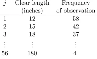
The demand schedule for a cutting job is given through a “cutbill”. A sample cutbill is shown in table 1.1. In this table, p is the index of each cut-piece type and “demand” is the required number of pieces of each type. Notice that each type of cut-piece has a distinct length; and obviously the length of cut-cut-pieces of the same type is the same.

(13)

Table 1.1: A sample cutbill

p Length Demand (inches)

1 14 1,800

2 25 1,500

3 33 1,650

4 40 1,000

Table 1.2: A sample frequency table of clear pieces

j Clear length Frequency (inches) of observation

1 12 58

2 15 42

3 18 37 ..

. ... ...

56 180 4

(14)

When we process the incoming strips (i.e. as we remove the defected areas), the resulting clear pieces have di¤erent lengths, and these clear pieces arrive at the crosscutting operation in a random manner. Each clear piece is cut according to a determined pattern after it arrives at the crosscutting operation. We can, therefore, approximate the expected amount (linear feet) of incoming strips required to satisfy demand for all cut-piece types using the expected number of clear pieces in the incoming strips. We assume that the expected number of clear pieces of a speci…c length in the incoming strips is proportional to the total length of the incoming strips. Once the distribution of clear pieces is obtained for a sample of length L0_{, where} _L0 _{is relatively large, we can approximate the expected}

number of clear piecej in the total lengthLof incoming strips. Leta0_j denote the observed number of clear piecej inL0 forj = 1; : : : ; J. It follows that the expected number of clear piece j inL, denoted by aj, can be approximated by the following equation.

aj

L

L0a0j (1.1)

We are now prepared to de…ne the crosscutting problem:

Given a cutbill withP distinct cut-piece types and the associated demands, and a frequency distribution of clear pieces in incoming strips as depicted byL0 anda0_j, determine a cutting pattern for each clear piecej, forj= 1; : : : ; J, so that the corresponding expected number of cut-pieces of each type obtained is at least as large as the corresponding demand for that cut-piece type and the expected total amount (linear feet) of incoming strips is minimized.

(15)

of the clear piece j for each p = 1; : : : ; P (i.e. a cutting pattern for the clear piece j), for

j = 1; : : : ; J, and the expected total length of the strips required to satisfy the demand

for all cut-piece types. Note that in this context once we decide on a cutting pattern for a particular clear piece, all incoming clear pieces of the same length are cut according to the same cutting pattern. The process of cutting incoming the clear pieces is continued until demand for all cut-piece types are satis…ed.

1.2

Organization of the Thesis

So far we have de…ned the crosscutting problem in this chapter. In chapter 2 we brie‡y review the related literature.

(16)

(17)

Chapter 2

Related Literature

In the sense of the basic principles, crosscutting problem is very similar to the cutting-stock problem (CSP). CSP was one the …rst applications of linear and integer pro-gramming, and this subject has been extensively treated in the open literature. It has a large variety of applications in industry such as steel, glass or wood cutting manufacturing. Lots of e¤orts have been dedicated to solving the CSP e¢ ciently.

(18)

2.1

Cutting Stock Problems

CSP is one of the combinatorial optimization problems which is de…ned as the problem of …nding geometrical cutting patterns for raw material (called objects or stock) so as to …ll an order of items at the minimum cost of the underlying process. This problem attracted lots of research interests over the last 50 years, mainly because of the large number of applications that it has. Lirov [8] presents a survey on (one-dimensional, two-dimensional, and three-dimensional) CSP, and reviews the possible approaches proposed for solving CSP. Hinxman [9] also performed a survey in this area with the focus on trim loss. Dyckho¤ and Finke [4] gathered a bibliography on cutting and packing problems. In this book, a complete de…nition of CSP and di¤erent aspects of it are presented. Below is the most important aspects of CSP

Dimensionality Pattern restriction Objectives

(19)

process has been reduced to two one-dimensional CSP by separating the ripping and cross-cutting processes.

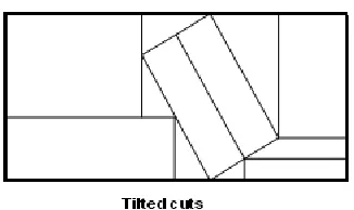
Pattern restriction is another issue which arises in the CSP. Orthogonal and non-orthogonal cuts are two main types of cutting pattern. Orthogonal cuts contain guillotine cuts which are the most common type of cutting pattern. In guillotine cuts all cuts are started from one edge of the object and continued to the opposite edge of it. Guillotine cuts can be categorized into three di¤erent types of single-stage, two-stage and three-stage. Figure 2.1 shows the orthogonal cuts including all types of guillotine cuts. In non-orthogonal cuts, shown in …gure 2.2, items may have angles with edges of objects. In crosscutting problem all cuts are single-stage orthogonal cuts. Cutting lumber into cut-pieces is a two-stage orthogonal cut, which is separated to two one-two-stage orthogonal cuts by performing ripping and crosscutting separately.

Objective is the other key issue which must be determined for the crosscutting problem. Some common objectives, listed in [4], are as follows:

Input minimization: Minimizing the number (or amount) of objects (and/or row material) used.

Trim loss minimization

–Trim loss minimization (absolute): minimizing trim loss quantity.

–Trim loss minimization (relative): minimizing trim loss quantity in relation to input quantity.

(20)

Figure 2.1: Orthogonal (and guillotine) cuts

(21)

Change-over minimization: Minimizing cost for altering cutting facilities.

Inventory cost minimization: Minimizing the (cost of) stock of objects and items. Value maximization: Maximizing the value of obtained items.

In the crosscutting problem we considered input minimization as our objective (which implies cost minimization).

2.2

Proposed Methods for Solving the Cutting Stock

Prob-lems

As we discussed in the previous section, crosscutting problem is a one-dimensional CSP. In this section we review the most common methods proposed for solving the CSP, but we focus our discussion on the methods proposed for solving one-dimensional CSP.

Assume there are available objects (stock) of length L. Note that unlike the crosscutting problem, in CSP we assume that all objects (which are clear pieces in the crosscutting problem) have identical length L. In one-dimensional CSP we want to cut the available stock (of identical length) such that an order consisting of m items is satis…ed. Let li, andNi, for each i= 1; : : : ; m, denote the length and the requested number of item

i; respectively. The one-dimensional CSP can now be de…ned as …nding cutting patterns for the available stock so as to satisfy the order according to an objective (which is usually de…ned as minimizing the cost or minimizing the trim loss). Let J denote the set of all possible cutting patterns, and aij denote the number of items iobtained from each object

(22)

problem, one-dimensional CSP is formulated as follows

Min X

j2J

xjvj

s.t X

j2J

xjaij Ni i= 1; : : : ; m

xj 0 j= 1; : : : ; J and Integer

(2.1)

wherevjis the trim loss associated with thejth cutting pattern (clearlyvj =L Pm_i₌₁liaij),

and xj, for j = 1; : : : ; J, is the number of objects (clear-pieces) cut according to the jth

cutting pattern.

The most common approach for solving the CSP is the linear programming (LP) approach which was …rst proposed by Gilmore and Gomory [7]. The objective that they considered for the CSP was minimizing the cost (or minimizing the total number of the required stock, assuming that there is unique price for each object). The model they developed for the CSP is as follows:

Min X

j₂J

cxj

s.t X

j2J

xjaij Ni i= 1; : : : ; m

xj 0 j= 1; : : : ; J

(2.2)

where c is the price of each object. Notice that the objective function could be replaced with “Min P_j₂_Jxj”, since c is a constant. Also notice that in model 2.2 the integrality

constraints are relaxed. In the LP approach, the LP relaxation (the model obtained by relaxing the integrality constraints on variables) of the problem is considered, and solved instead; then a rounding procedure is used to get an integer solutions.

(23)

by Gilmore and Gomory [7] was developed to overcome this di¢ culty. In this method, the cutting patterns are generated during the process of solving the problem through an auxiliary problem. The method starts with a set of simple patterns (to form the initial basis), then the solution is improved by removing a cutting pattern and generating a new one (same as pivoting procedure in simplex; the cutting pattern which is removed is the leaving variable and the new cutting pattern is the entering variable). The new cutting pattern is generated using the auxiliary problem which is easy to solve; knapsack problem normally serves as the auxiliary problem, and there are several methods for solving this problem. The new column is generated in a manner that it results in the most possible improvement in the solution (based on the same concept as choosing the entering variable to be the nonbasic variable with the most negative reduced cost in the simplex method). The column generation method is summarized below.

1. Initialize the procedure: Let B; the basis matrix, be a collection of some simple (feasible) patterns.

2. Solve the following (auxiliary) problem:

Max CBB 1A

s.t lTA L

A 0 and Integer

(2.3)

where CB (vector of cost coe¢ cient of the basic variable); and B 1 (inverse of the

basic matrix) are known;Ais a (column) vector which contains the decision variables of the problem;lis a vector equal to(l1; : : : ; lm)T; andLis a constant. LetA denotes

the optimal solution of problem 2.3.

(24)

reduced costs, c CBB 1A , are non negative for all non basic variables).

4. If CBB 1A > c, thenA enters the basis (since we maximized CBB 1A, A is the

most pro…table cutting pattern, i.e. it has the most negative reduced cost). 5. Find the leaving variable by the ratio test.

6. Form the new basis, and go back to 2.

Column generation method is discussed in more detail in [7], chapter 11 of [14], and chapter 13 of [2]. After Gilmore and Gomory proposed the column generation method, many researchers used it for their CSP problems. Seth [11] used it for a wood cutting problem, which is similar to crosscutting problem that we discuss later. However in the problem that seth considered the di¤erence of the objects are their thickness, and in the problem that he considered there are only two di¤erent thickness. But in the crosscutting problem we deal with a large number of clear pieces.

Lirov [9] mentioned enumerative approach as another approach for solving the CSP in his survey. Enumerative approach contains discrete optimization methods such as branch and bound or dynamic programming or a combination of these two.

(25)

feasible region into smaller sets; computing the (lower or upper) bounds; and eliminating the sets which can not make any improvement in the solution (having a worse bound than the current solution). Obviously the procedure stops when all the remaining subsets have been shown to contain no better option. See [14] for more information on the basic principles of branch and bound and dynamic programming method.

DP is the most common enumerative method, used for solving CSP. In this method the objective of the problem is normally considered to be maximizing the total obtained value. A value is assigned to each item; each incoming object is cut in a manner that the total obtained value is maximized. Sarker [10] used this approach for solving one-dimensional CSP. It is also noticeable that possible defects are also considered in this paper. In this paper having defects in items are acceptable, but defected items have less value.

Besides all the exact methods reviewed so far, there are a large number of inexact (heuristic) methods for the CSP. Seth et al. [12] developed a heuristic for one-dimensional CSP. Vahrenkamp [13] proposed an interesting heuristic based on the packing concepts for the CSP. Chen et al. [3] presents a simulated annealing procedure for the CSP.

(26)

Chapter 3

An MIP Model for the

(27)

inequalities (as compared with that of the original model). Results of this experiment are presented in section 3.4.

3.1

A Mixed Integer Programming (MIP) Model

In this section we present a MIP model for the crosscutting problem. First in subsection 3.1.1 we introduce the notations used in the model. The MIP model is presented later in subsection 3.1.2.

3.1.1 Notation

The notations used in the model are as follows:

Input Parameters

rp :Length of cut-piece typepin the cutbill (p= 1 P).

dp :Demand for cut-piece typep(p= 1 P).

hj :Length of the clear piece j (j= 1 J).

L0_:_{Total length of strips for a speci…c sample}

a0_j :Frequency (i.e. number of occurrence) of clear piece j in the sample.

Outputs

–Decision Variables

xjp :Number of cut-pieces of type pcut out of a clear piece j.

(28)

3.1.2 The Model

Two sets of constraints must be satis…ed in the crosscutting problem. First set of constraints ensures the total length of all cut-pieces cut out of each clear piece does not exceed the length of that clear piece, and the second set of constraints enforces demand satisfaction for all cut-piece types. We call these sets of constraints the “length constraints” and the “demand constraints”, respectively.

The length constraints can be written as

P

X

p=1

rpxjp hj j= 1; : : : ; J (3.1)

To write the demand constraints we need to make sure that the expected number of cut-pieces of type p produced by cutting the total length L of strips is greater than or equal todp. As mentioned in chapter 1, the expected number of clear piecesj inL,aj, can

be approximated as

aj

L

L0a0j j= 1; : : : ; J: (3.2)

For eachp= 1; : : : ; P; we de…nenp as the total number of cut-pieces of type pexpected to

be obtained after crosscutting the length L of the incoming strips. It follows that np can

be written as

np=

J

X

j=1

ajxjp p= 1; : : : ; P: (3.3)

(29)

np J

X

j=1

L

L0a0jxjp p= 1; : : : ; P: (3.4)

Therefore the demand constraints can be written as

J

X

j=1

L

L0a0jxjp dp p= 1; : : : ; P: (3.5)

The objective is to minimize L. Putting all the constraints and the objective together, the MIP model can be written as follows:

Min L

s.t.

P

X

p=1

rpxjp hj j= 1; : : : ; J

J

X

j=1

L

L0a0jxjp dp p= 1; : : : ; P

xjp 0 Integer

j= 1; : : : ; J

p= 1; : : : ; P

(3.6)

Model 3.6 is not linear because of its demand constraints. Let us introduce a new notation

L, de…ned as L = 1

L. We can now transform model 3.6 to a linear form using L. The

objective function of model 3.6 can be properly changed to maximizingL, since minimizing

L is equivalent to maximizing L. Demand constraints can now be described by linear inequalities as shown below

Max L

s.t

P

X

p=1

rpxjp hj j = 1; ; J

J

X

j=1

a0

j

L0xjp Ldp p= 1; ; P

xjp 0 Integer j = 1; : : : ; J

p= 1; : : : ; P

(3.7)

(30)

3.6 and the corresponding constraints are similar. The number of variables and constraints in this model are J P and J+P, respectively.

3.2

Experimental Analysis of the MIP Model

In this section we experiment with model 3.7 by solving several instances of the problem. We also analyze the results of these experiments. AMPL is used as the mathe-matical programming language to code the model and CPLEX is used as the solver. We present the AMPL-CPLEX code and list of the commands that we used in appendix A.

In the next subsection we explain how the instances of the experiment are con-structed. In subsection 3.2.2 we describe the main features of CPLEX related to the imple-mentation of the experiment. We bring the results and the observations on the experiment in subsection 3.2.3.

3.2.1 Data Sets

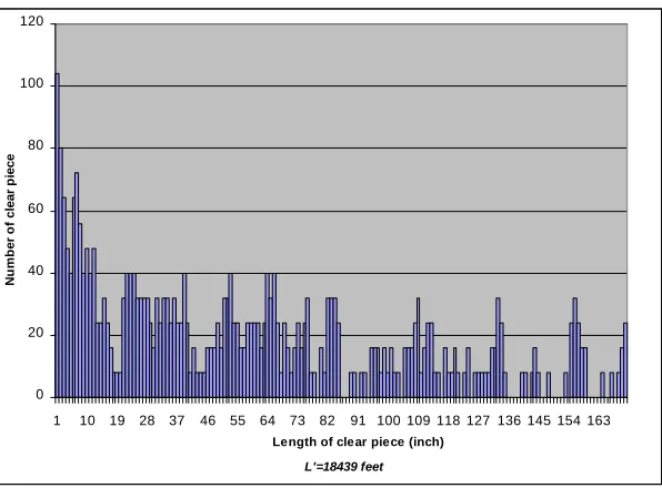
To solve the model with AMPL-CPLEX, parameters of the model must be de…ned in a data …le (.dat …le). These parameters include those mentioned in chapter 1. A frequency distribution was obtained from a sample at a local manufacturing plant and used throughout the experiment. This frequency distribution is shown in …gure 3.1 (at one inch intervals).

(31)

0 20 40 60 80 100 120

1 10 19 28 37 46 55 64 73 82 91 100 109 118 127 136 145 154 163

Nu

m

b

er

o

f clear

p

iece

Length of clear piece (inch) L'=18439 feet

Figure 3.1: Clear pieces distribution

inches. The range for the clear lengths can vary depending on the instances; however we use the range of 13 to 183 inches in this thesis.

(32)

the frequency distribution. In …gure 3.1 we have = 1.

We generated three cutbills with P = 4, 7, and 10, respectively. Let us call the cutbill with 4 cut-piece types CB3-1, the cutbill with 7 cut-piece types CB3-2, and the cutbill with 10 cut-piece types CB3-3. In each of these cutbill, the length of each type of cut-piece is obtained randomly using a uniform distribution between 13 and 98 inches, where 98 is the middle point between the maximum and the minimum clear lengths in our frequency distribution. Demand for each type of cut-piece is also generated randomly using a uniform distribution between 1000, and 3000. These cutbills are presented in appendix B.

(33)

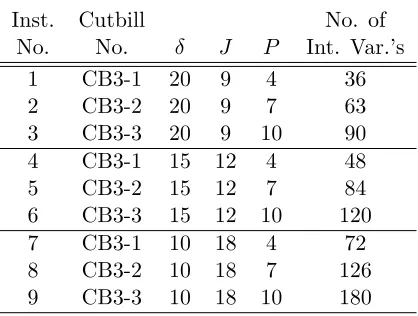
Table 3.1: Constructed instances Inst. Cutbill No. of

No. No. J P Int. Var.’s 1 CB3-1 20 9 4 36 2 CB3-2 20 9 7 63 3 CB3-3 20 9 10 90 4 CB3-1 15 12 4 48 5 CB3-2 15 12 7 84 6 CB3-3 15 12 10 120 7 CB3-1 10 18 4 72 8 CB3-2 10 18 7 126 9 CB3-3 10 18 10 180

3.2.2 CPLEX Features

To solve the proposed MIP model we use CPLEX as the solver and branch and bound as the solving method. CPLEX is capable of deciding on many important aspects of solving a problem with branch and bound method such as the method of branching (i.e. breadth …rst or depth …rst or combination of these two), the variable to branch on, the method of solving the LP relaxation problem of a node, and whether or not to add one of the well-known cuts (such as Gomory’s MIR cuts or Gomory’s fractional cuts) at each node. We use the default values of CPLEX for the priority rule, branching variable, and the method to solve the LP relaxation; however we would like to study the e¤ect of cuts added to the model, since it is also related to the topic of our next section. As a result each instance of the problem has been solved in two di¤erent conditions. In the …rst case no cuts are allowed to be added to the model, and in the other case the default cuts of CPLEX are allowed to be added to the model.

(34)

(depending on the instance of the problem) in order to avoid numerical di¢ culty.

3.2.3 Results and Observations

Our major purpose of the performed experiment is to …gure out the relation be-tween the size of an instance and the computational e¤ort required to solve it. This gives the insight as to whether the MIP model is capable of solving the realistic sized instances of the problem. Since the overall computational requirement of the branch and bound al-gorithm is directly related to the number of nodes in B&B tree, we consider the “number of nodes” as a measure for evaluating the model. Other important issues are “CPU time” and “number of MIP simplex iterations”.

As we mentioned in previous section, in the instances that we consider in this experiment is as large as 20 inches, 15 inches, or 10 inches; however in reality could be equal to an inch or a fraction of an inch (up to ₁₆1 inch) as discussed in chapter 1. Another purpose of performing the experiment is to observe the relationship between and L(total amount (linear feet) of strips required). To this end, we compare the required length of incoming strips (L) obtained from solving each cutbill with each frequency distribution (resulted from changing ), and study the trend ofL as decreases.

(35)

Table 3.2: Experiment results when CPLEX adds no cuts

Inst. Cutbill No. of No. of No. of CPU Time No. No. J P Int. Var.’s Nodes MIP Simplex It. (seconds)

1 CB3-1 20 9 4 36 9 33 0.001

2 CB3-2 20 9 7 63 6,823 11,992 0.609 3 CB3-3 20 9 10 90 59,877 141,895 7.046

4 CB3-1 15 12 4 48 11 49 0.015

5 CB3-2 15 12 7 84 38,428 165,039 7.953 6 CB3-3 15 12 10 120 6,660,362 19,009,951 1,444.593

7 CB3-1 10 18 4 72 33 70 0.001

8 CB3-2 10 18 7 126 1,165,015 3,770,369 175.625 9 CB3-3 10 18 10 180 23,670,341 141,236,093 7,541.22

We can observe that number of nodes increases sharply when the size of the prob-lem gets large either by increasing the number of cut-piece types or by decreasing which results in increasing the number of clear pieces. The same pattern is also observable in number of MIP simplex iterations and the CPU time. The increase rate is so steep that for instance 9 the solver processed 23,670,341 nodes, and the solving time for this instance is about 120 minutes, while in this instance is equal to 10 inches, which is still relatively large.

(36)

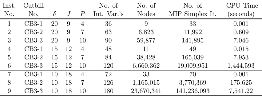
Table 3.3: Number of nodes vs. number of clear pieces and number of cut-pieces

J

P _# 9 12 18

4 9 11 33

7 6,823 38,428 1,165,015 10 59,877 6,660,362 23,670,341

-1 4 9 14 19 24

0 50 100 150 200

M

illio

n

s

number of integer variables

J=9 N um be r of node J=12 J=18

Figure 3.2: Number of nodes vs. number of integer variables

for the latter instance is about six times of the number of nodes for the former instance. Table 3.3 is depicted in …gure 3.2. There are three lines in the …gure, each of which corresponds to a column of table 3.3. The horizontal line shows the number of integer variables, and the vertical line shows number of nodes in millions.

As we previously mentioned, our analysis consists of another part which is studying the e¤ect of decreasing onL(the expected total required length of incoming strips). Table 3.4 summarizes L (1

L; where L is the objective value of model 3.7) for each instance. In

(37)

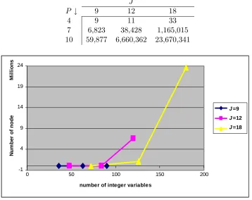
Table 3.4: Required length of incoming strips Inst. Cutbill L

No. No. J P (Linear feet) 1 CB3-1 20 9 4 31,021 2 CB3-2 20 9 7 52,572 3 CB3-3 20 9 10 82,202 4 CB3-1 15 12 4 30,057 5 CB3-2 15 12 7 48,041 6 CB3-3 15 12 10 79,254 7 CB3-1 10 18 4 28,535 8 CB3-2 10 18 7 46,559 9 CB3-3 10 18 10 77,573

Table 3.5: Required length of incoming strips vs. aggregation parameter % reduction in

P _# 20 15 10 optimal value of L

4 31,021 30,057 28,535 8.01 7 52,572 48,041 46,559 11.44 10 82,202 79,254 77,573 5.63

We can observe that for each cutbill the corresponding optimal value ofLdecreases as decreases. The last column in table 3.5 shows the percentage reduction in the optimal value of Lfor each instance as we decrease the corresponding value of from 20 to 10. We can observe that in these instances total amount of incoming strips (L) is reduced by up to 11%when the aggregation parameter ( ) is reduced from 20 inches to 10 inches. Naturally if we further reduce the value of the corresponding optimal value of L would also reduce further. This trend is depicted in …gure 3.3, for = 20;15;and 10.

(38)

20000 30000 40000 50000 60000 70000 80000 90000

5 7 9 11 13 15 17 19 21

P=4

P=7

P=10

L

(l

in

ear

feet)

Figure 3.3: Total incoming strips vs. aggregation parameter

CPLEX cuts and other proper valid inequalities to the model.

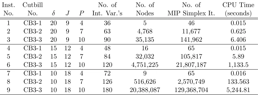
To study how much the computational e¢ ciency of the model can improve by adding the proper cuts to the model, we re-solve the same instances using the same model, and this time we use CPLEX default settings. Using the default settings of CPLEX, the solver is allowed to add cuts to the model when it is applicable. Table 3.6 summarizes the results obtained from solving the same instances by the proposed MIP model and CPLEX when adding the default cuts by CPLEX is allowed.

(39)

Table 3.6: Experiment results when CPLEX adds the default cuts

1 CB3-1 20 9 4 36 5 46 0.015

2 CB3-2 20 9 7 63 4,768 11,677 0.625 3 CB3-3 20 9 10 90 35,135 141,962 6.406

4 CB3-1 15 12 4 48 16 65 0.015

5 CB3-2 15 12 7 84 32,032 105,817 5.89 6 CB3-3 15 12 10 120 4,751,225 21,807,187 1,133.5

7 CB3-1 10 18 4 72 9 65 0.016

8 CB3-2 10 18 7 126 516,626 2,570,749 133.563 9 CB3-3 10 18 10 180 20,388,087 129,368,704 5,244.81 the last two tables, we expect that the number of nodes becomes incredibly larger when the size of the instance becomes larger.

Adding cuts may not be helpful for all instances. Among the collection of 9 instances reported in table 3.6, we can observe that for instance 4 the added cuts caused an increase in the number of nodes and the corresponding number of simplex iterations. However for other instance, especially for the large instances, added cuts were generally useful. The observed deterioration in the performance of the model for small instances is potentially due to the fact that adding cuts enlarges the size of the LP relaxation problem at each node. Thus the MIP simplex iterations and the corresponding time to solve the LP relaxation of each node increase. The increase in number of nodes is harder to explain and it could be due to chance causes.

(40)

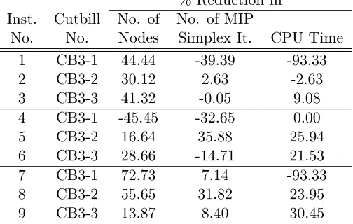
Table 3.7: Computational e¢ ciency improvement after using default cuts of CPLEX % Reduction in

Inst. Cutbill No. of No. of MIP

No. No. Nodes Simplex It. CPU Time 1 CB3-1 44.44 -39.39 -93.33 2 CB3-2 30.12 2.63 -2.63 3 CB3-3 41.32 -0.05 9.08 4 CB3-1 -45.45 -32.65 0.00 5 CB3-2 16.64 35.88 25.94 6 CB3-3 28.66 -14.71 21.53 7 CB3-1 72.73 7.14 -93.33 8 CB3-2 55.65 31.82 23.95 9 CB3-3 13.87 8.40 30.45

Graph 3.4, which visualizes table 3.7, may give a better intuition about the reduc-tion in the computareduc-tional e¤ort required to solve the problem when the cuts are allowed to be added. The horizontal axis of the chart shows number of nodes for the case of having no added cuts, and the vertical axis shows number of nodes for the case of having proper cuts. Line x = y is also drawn in the graph. The graph is in logaritmic scale on both axes; hence the magnitude of the physical distance along the two axes should be interpreted accordingly. It is obvious that a dot below the line shows an improvement (in terms of the number of nodes) for that particular instance after adding the cuts.

(41)

1 10 100 1000 10000 100000 1000000 10000000 100000000

1 10 100 1000 10000 100000 1000000 1E+07 1E+08

Number of nodes for the MIP model

N um be r of node s f or th e M IP mo d e l w it h Va lid In e q u a lit ie s

Figure 3.4: Number of nodes with no cuts vs. number of nodes with default cuts

valid inequalities that we propose for this MIP model are introduced and the e¤ect of these valid inequalities on the computational e¢ ciency of the model is studied.

3.3

Developing Valid Inequalities

(42)

3.2 and the e¤ect of these additional valid inequalities on the computational e¢ ciency of the model is studied.

3.3.1 Valid Inequalities

The valid inequalities we propose in this section deal with the length constraints of model 3.7. Length constraints are as follows:

P

X

p=1

rpxjp hj j= 1; : : : ; J

The above set of constraints representsJ separable constraints, each of which stands for one of the clear lengths. We propose P distinct valid inequalities for each of these constraints. These valid inequalities are based on the fact that due to the length restriction of each clear piece, the maximum number of obtainable cut-pieces out of that clear piece is limited. These valid inequalities are akin to the cover inequalities in the context of the knapsack constraints. The general form of the proposed valid inequalities for the jth constraint in the group and for each value ofi_{2 f}1; : : : ; P_g is as follows:

P

X

p=i

xjp kij i= 1; : : : ; P and j= 1; : : : ; J (3.8)

in which kij is an integer number equal to the maximum number of cut-pieces of type

i; i+ 1; : : : ; P obtainable from the clear-piecej. Informally the preceding constraints means

that at most kij cut-pieces of lengths ri; ri+1; : : : ; rP can be produced from a clear-piece

with lengthhj .

(43)

rep-resent the constant kij simply as k. Its dependence on i and j is clear from the context.

Let us start our discussion with i= 1. So for a speci…c value of j we want to …nd k such that constraint PP_p₌₁xjp k is a valid inequality for model 3.7. It is obvious that the

maximum number of cut-pieces from each clear piece is obtained when we cut only the shortest cut-piece out of that clear piece. Therefore the value ofk associated with the jth clear piece can be obtained as follows:

k= hj=min

P frpg (3.9)

Without loss of generality, let us assume rp’s are ordered in nondecreasing order (i.e. r1

r2 rp). As a result for each value of j, and for i = 1, the corresponding value of

k can be rewritten as k = _bhj=r1c:Thus the collection of all valid inequalities associated

withi= 1 for all values ofj can be written as

P

X

p=1

xjp

hj

r1

j= 1; : : : ; J (3.10)

We now discuss the valid inequalities corresponding toi= 2. Recall the constraint

PP

p=1rpxjp hj, which is the length constraint of model 3.7. Since xj1 0, we can

relax the constraint to get the new constraint PP_p₌₂rpxjp hj. Same procedure can

be repeated on the new constraint to get the new valid inequality PP_p₌₂xjp

j_h j

r2

k

, for

each j = 1; : : : ; J. We can now state the general form of the valid inequality for each

i= 2; : : : ; P, and for each j= 1; : : : ; J. We …rst relax the corresponding length constraint

by removing _fxj1; : : : ; xj(i 1)g, and then we obtain the corresponding valid inequality in

(44)

inequalities, for i= 1; : : : ; P, is as follows:

P

X

p=i

xjp

hj

ri

j= 1; : : : ; J (3.11)

The MIP model after the addition of all valid inequalities is shown below

Min L

s.t.

P

X

p=1

rpxjp hj j= 1; ; J

P

X

p=i

xjp

hj

rp

i= 1; : : : ; P 1; j= 1; ; J

J

X

j=1

a0_j

L0xjp Ldp p= 1; ; P

L 0

xjp 0 Integer

(3.12)

Valid inequalities are shown in model 3.12 after the length constraints. In the next section a similar experiment to that performed in section 3.2 is repeated for the MIP model with the valid inequalities; and the results are compared with those in section 3.2.

3.4

Experimental Analysis of the MIP Model with Valid

In-equalities

(45)

Table 3.8: Experiment results with VI’s when Cplex adds no cuts

1 CB3-1 20 9 4 36 15 45 0.001

2 CB3-2 20 9 7 63 4,539 10,390 0.578 3 CB3-3 20 9 10 90 24,492 98,119 4.593

4 CB3-1 15 12 4 48 7 32 0.001

5 CB3-2 15 12 7 84 24,933 67,282 2.984 6 CB3-3 15 12 10 120 3,717,178 183,657,704 844.593

7 CB3-1 10 18 4 72 21 71 0.015

8 CB3-2 10 18 7 126 336,993 1,482,911 82.484 9 CB3-3 10 18 10 180 18,506,854 128,503,804 5,082.48

The results of solving the instances with MIP model 3.12 (MIP model with the valid inequalities) and CPLEX (when no additional CPLEX cuts are added to the model) are presented in table 3.8. Consistent with our expectation the number of nodes, the number of MIP simplex iterations, and the CPU solving time increase as the size of the problem gets large. Comparing the results of table 3.8 and those of table 3.2, we observe that on average the valid inequalities improve the computational e¢ ciency of the model signi…cantly. Table 3.9, summarizes the e¤ect of the valid inequalities on the performance of the model (using the results of tables 3.8 and 3.2). The format of this table is similar to that of table 3.7 (i.e. values are % reduction in corresponding measures after adding the valid inequalities 3.11 to the model 3.7).

(46)

Table 3.9: Computational e¢ ciency improvement by the VI’s when CPLEX adds no cuts % Reduction in

No. No. Nodes Simplex It. CPU Time 1 CB3-1 -66.67 -36.36 0.00 2 CB3-2 33.48 13.36 5.09 3 CB3-3 59.10 30.85 34.81 4 CB3-1 36.36 34.69 93.33 5 CB3-2 35.12 59.23 62.48 6 CB3-3 44.19 3.39 41.53 7 CB3-1 36.36 -1.43 -93.33 8 CB3-2 71.07 60.67 53.03 9 CB3-3 21.81 -9.01 32.60

the number of nodes. So adding the valid inequalities in some instances can increase the computational e¤ort required to solve the problem by increasing the number of constraints and therefore enlarging the size of the LP relaxation of the model.

Graph 3.5 may give a better understanding about the strength of valid inequalities. It shows the number of nodes when the instances are solved in two cases of solving the problem with model 3.7 and model 3.12 when no cuts are added to the model by CPLEX. The format of the graph is similar to that of …gure 3.4.

Comparing tables 3.8 and 3.6, it is also noticeable that valid inequalities could improve the computational e¢ ciency of the model more than the cuts added by CPLEX. To see whether the valid inequalities could be e¢ cient after adding the cuts of CPLEX, same steps as above are followed when adding cuts by CPLEX is also allowed. Table 3.10 shows the result of solving the MIP model with valid inequalities when adding cuts by CPLEX is also allowed.

(47)

1 10 100 1000 10000 100000 1000000 10000000 100000000

1 10 100 1000 10000 100000 1000000 1E+07 1E+08

Number of nodes for the MIP model

N um be r of node s f or th e M IP mo d e l w it h Va lid In e q u a lit ie s

Figure 3.5: Number of nodes with VI’s vs. without VI’s when CPLEX adds no cuts

Table 3.10: Experiment results with VI’s when Cplex adds the default cuts Inst. Cutbill No. of No. of No. of CPU Time

No. No. J P Int. Var.’s Nodes MIP Simplex It. (seconds)

1 CB3-1 20 9 4 36 0 23 0.001

2 CB3-2 20 9 7 63 5,941 23,961 1.312 3 CB3-3 20 9 10 90 59,588 414,844 18.125

4 CB3-1 15 12 4 48 6 47 0.015

5 CB3-2 15 12 7 84 11,711 77,061 3.719 6 CB3-3 15 12 10 120 2,443,930 11,962,879 691.968

7 CB3-1 10 18 4 72 20 64 0.015

(48)

Table 3.11: Computational e¢ ciency improvement by the VI’s in addition to CPLEX cuts % Reduction in

No. No. Nodes Simplex It. CPU Time 1 CB3-1 100.00 50.00 93.33 2 CB3-2 -24.60 -105.20 -109.92 3 CB3-3 -69.60 -192.22 -182.94 4 CB3-1 62.50 27.69 0.00 5 CB3-2 63.44 27.18 36.86 6 CB3-3 48.56 45.14 38.95 7 CB3-1 -122.22 1.54 6.25 8 CB3-2 41.28 47.53 39.39 9 CB3-3 12.13 8.78 7.86

improvement in computational e¢ ciency of the model obtained from the valid inequalities in addition to the improvement resulted from CPLEX cuts.

Table 3.11 shows that additional valid inequalities indeed strengthen the LP bound and therefore reduce the number of node, although this is not a general rule as it is not true for the small instances. They may, however, increase the number of MIP simplex iterations by enlarging the LP relaxation of the problem.

(49)

(50)

Chapter 4

A Heuristic Algorithm for the

In this chapter we propose a heuristic method for solving the crosscutting problem. In the last chapter we presented a MIP model for this problem. Crosscutting problem could be solved optimally using this MIP model. However, as mentioned earlier, its computational requirement is excessive for large instances of the problem. This raises the necessity of …nding a fast method for solving the problem. As a result we propose a heuristic method for solving the problem quickly, although we can not guarantee that it …nds an optimal solution.

(51)

it is not more than its length; in other words a solution is called feasible when it satis…es the length constraints.

The proposed heuristic is an iterative procedure. We de…ne one parameter as-sociated with each cut-piece type, and we refer to this parameter as the “coe¢ cient” for that cut-piece type. We use these coe¢ cients in the context of the heuristic procedure to determine the cutting pattern xjp. Our objective is to determine the coe¢ cients so as

to minimize the expected total length of incoming strips required to satisfy demand of all cut-piece types. To this end, our heuristic procedure attempts to maximize the minimum of these coe¢ cients. We will later show that under certain condition maximizing the minimum coe¢ cient is equivalent to minimizing the expected total length of the incoming strips. Each iteration starts with a feasible solution. Coe¢ cients of all cut-piece types are calculated using the current solution (xjp’s). Subsequently the feasible solution is changed in a

man-ner that the feasibility of the solution is maintained and the minimum coe¢ cient steadily increases.

As we will show later, once we know a solution, we can then …nd the expected total length of the incoming strips required to satisfy the demand for all cut-piece types (using the coe¢ cients corresponding to that solution). In practice, however, the incoming clear pieces are cut according to the cutting patterns (de…ned by the solution) until demand for all cut-piece types are actually satis…ed. We will show that the total amount of incoming strips expected to be consumed to satisfy the demand for all cut-piece types is the inverse of the minimum coe¢ cient corresponding to the solution (cutting patterns) which is used.

(52)

The heuristic algorithm is presented in section 4.2. In section 4.3 we discuss how the pro-posed heuristic solves the crosscutting problem. Section 4.4 ends this chapter by evaluating the heuristic method empirically.

4.1

Notation and Terminology

In addition to the notation and terminology introduced earlier, we introduce sev-eral new terms that are speci…cally used in the context of the heuristic algorithm that we propose. For completeness we review the previous notation before introducing the new terminology.

Input Parameters

rp :Length of cut-piece typepin the cutbill (p= 1 P).

dp :Demand for cut-piece typep(p= 1 P).

hj :Length of the clear piece j (j= 1 J).

L0:Total length of strips for a speci…c sample

a0

j :Frequency (i.e. number of occurrence) of clear piece j in the sample.

Outputs

–Decision Variables

xjp :Number of cut-piecesp cut out of a clear piecej.

(53)

4.1.1 New Terminology

Below are the new terms that we de…ne in the context of the heuristic, in addition to the terms that we de…ned earlier.

De…nition 1 Waste of clear piece typej, denoted bywj, is the unused length of clear piece

j in the current solution. We de…newj mathematically by the following equation

wj =hj

P

X

p=1

rpxjp j = 1; : : : ; J (4.1)

In the last chapter, we introduced the length constraints as follows:

P

X

p=1

rpxjp hj j= 1; : : : ; J

and we referred to every solution that satis…es this constraint as a “feasible solution”. This inequality can be written as

hj

P

X

p=1

rpxjp 0 j = 1; : : : ; J (4.2)

By de…nition, the left hand side of this inequality is wj. Therefore we can now de…ne

feasibility of a solution in terms of wj’s as follows:

wj 0 j= 1; : : : ; J (4.3)

De…nition 2 Coe¢ cient of cut-piece typep, denoted bycp, is the total number of cut-pieces of type p cut out of one linear foot of the incoming strips (i.e.

PJ j=1a0jxjp

(54)

demand for that cut-piece type (i.e. dp). The coe¢ cientcp can be obtained by the following equation mathematically.

cp=

PJ

j=1 a0

j

L0xjp

dp

p= 1; : : : ; P (4.4)

or

cp=

PJ

j=1a0jxjp

L0_d_p p= 1; : : : ; P (4.5)

From equation 4.5 it is obvious that for each p the corresponding value of cp

changes whenever xjp, for any j = 1; : : : ; J, changes. Therefore we have a distinct set of

values for the coe¢ cientscp’s corresponding to each solutionxjp’s. We will later show that

associated with each solution (cutting pattern), the expected total length of the incoming strips required to satisfy the demand for cut-piece type p is equal to _c1

p. It follows that

the expected total length of incoming strips required to satisfy the demand for all cut-piece types is equal to max

p=1;:::;Pf 1 cpg:

4.2

The Heuristic Algorithm

Below is the outline of the heuristic algorithm that we propose. We …rst present the algorithm, and then we explain each of its steps. We refer to this algorithm as algo-rithm 1. For convenience in presentation, without loss of generality we make the following assumptions:

(55)

Clear pieces are in nondecreasing order of their frequency (i.e. a0₁ a0₂ : : : a0_J).

Algorithm 1

1. Initialization step of the algorithm:

(a) Randomly generate a feasible solution (a solution which does not violate length constraints PP_p₌₁rpxjp hj), i.e., for each clear length j determine a cutting

pattern (xjp for p = 1; : : : ; P) that would satisfy its corresponding length

con-straint.

(b) Calculate cp’s forp= 1; : : : ; P using equation 4.4.

(c) Calculate wj’s forj = 1; : : : ; J using equation 4.1.

2. Iterative step of the algorithm: (this step is repeated while the stopping criteria is not satis…ed)

(a) Find the index of the minimum coe¢ cient. Assume the minimum coe¢ cient happens atq, i.e. cq = min

p fcpg.

(b) For all indices p= 1; : : : ; P andp₆=q, perform the following steps: i. For j= 1; : : : ; J, whilexjp>0 do the following steps:

A. Temporarily reduce xjp by 1, and calculate cp as cp a0_j

L0dp (notice that cp is the coe¢ cient of cut-piece typepif we permanently change current

xjp toxjp 1).

B. If cp > cq; permanently reduce xjp by 1. Replace cp by cp;and update

(56)

(c) Forj =J; : : : ;1 (we will describe the reason of the reversed order later), do the following steps:

i. Find the index of the minimum coe¢ cient (obviously the index of the mini-mum coe¢ cient isq when this step is performed for the …rst time but it may change when this step is repeated due to the fact that each time this step is performedcq increases as we will discuss later) ; if it still happens at q (i.e.

ifcq= min

p fcpg still holds) do the following steps; otherwise go to d:

A. Increase xjq, by

j_w

j

rq k

; let kdenote

j_w j

rq k

:

B. Replacecq by cq+ ka0

j

L0dq, and wj bywj krq:

(d) Forj= 1; : : : ; J, and p=P; : : : ;1, set xjp =

j_w j

rp k

; revisecp; revisewj.

3. Stopping criteria

The procedure stops when the same minimum coe¢ cient is repeated for a certain number (I0) of iterations.

In the …rst step of the algorithm, we initialize the algorithm by …nding an initial solution. The initial solution is a feasible solution which is generated randomly. Then we calculate coe¢ cients and wastes corresponding to the initial solution. Obviously wj 0;

forj= 1; : : : ; J, since the initial solution is a feasible solution.

(57)

The coe¢ cient of a cut-piece type is the ratio of the number of cut-pieces of that type produced in one linear foot of the incoming strips to the demand of that cut-piece type. When the coe¢ cient of a cut-piece type is small, it means that the ratio of the number of cut-pieces of that type produced to its demand is smaller than that of other cut-piece types; therefore it is desirable to increase the number of cut-pieces of that type that we produce. In the proposed heuristic we try to increase the number of cut-pieces of type q that we produce (the cut-piece type with minimum coe¢ cient) at each iteration. To this end at step 2(b) we reduce the number of cut-pieces of other types produced, and in step 2(c) we increase the number of cut-pieces of type q instead. In the next section we show how this procedure can actually reduce the expected total amount (linear feet) of incoming strips required to satisfy demand for all cut-piece types.

As mentioned above, step 2 contains two main blocks which are steps 2(b) and 2(c). The purpose of step 2(b) is to increase wj’s, so we can obtain more cut-pieces of

type q out of them in the next step (hence increasing the value of cq). In this step, for

p = 1; : : : P and p₆=q, we reduce xjp, for j = 1; : : : ; J; however, the reduction procedure

for eachp= 1; : : : ; P continues whilecp remains greater than cq:To do so, we …rst check to

see if cp > cq is satis…ed, wherecp is the coe¢ cient of cut-piece type p ifxjp decreases. If

cp > cq holds thenxjp is reduced andcp is replaced withcp:Notice that in this stepwj, for

j= 1; : : : ; J, increases if it changes at all, so the feasibility of the solution is not violated.

In step 2(c) cut-piece type q is cut out of the waste of each clear-piece whenever it is possible, i.e. xjq, for anyj= 1; : : : ; J, increases bykwherekis the largest integer less

than wj

rq (i.e. k= j_w

j

rq k

(58)

terminated whencq is no longer the minimum coe¢ cient. In 2(d) we simply obtain possible

cut-pieces out of the remaining length of each clear piece.

The reason that we assumed clear pieces are ordered in nondecreasing order of their frequency is to have a control on the decrease in the coe¢ cients of cut-piece type p;

forp= 1; : : : ; P andp₆=q, in step 2(b), and the increase of the coe¢ cient of cut-piece type

q in step 2(c). By this ordering, the reduction step is done as slow as possible, while the increasing step takes sharp steps. The reason that we used the reverse order in step 2(c) is that aJ aJ 1 a1 by the second assumption. If we want to increase cq such that

it will no longer be the minimum coe¢ cient, it is more desirable to usewJ, and thenwJ 1,

and so on.

Last step of the algorithm checks the termination criterion. The algorithm ter-minates when same minimum coe¢ cient is repeated for a certain I0 number of iterations.

Based on some experimental observations we decidedI0 to be 50. In next section we show

how the above algorithm could actually solve the crosscutting problem.

4.3

An Intuitive Argument for the Heuristic Algorithm

Algorithm 1 is obviously an iterative algorithm as mentioned. Below we …rst show that this algorithm keeps feasibility of the solution; then we show that maximizing the minimum coe¢ cient results in minimizing the total length of strips required to satisfy demand for all cut-piece types.

The algorithm starts with an arbitrary feasible solution (i.e. wj 0 for j =

(59)

for each j = 1; : : : ; J, wj decreases whenever xjp, for any p = 1; : : : ; P, increases. In the

above algorithm, only in step 2(c) xjq, for j = 1; : : : ; J, may increase. However, xjq, for

j = 1; : : : ; J, increases by k where k =jwj

rq k

; therefore wj krq = wj rq

j_w

j

rq k

remains nonnegative. So the feasibility of a solution is never lost through the above algorithm.

The above algorithm tries to maximize the minimum coe¢ cient by improving it in each iteration. First we explain how the minimum coe¢ cient increases in each iteration, then we present a lemma which shows how this helps to reduce the total required length of incoming strips. By de…nition, cp changes whenever xjp for any j = 1; : : : ; J changes.

At the beginning of each iteration the minimum coe¢ cient is equal tocq. Letcmin denotes

the minimum coe¢ cient at the beginning of each iteration; so cmin = cq. In step 2(b),

xjp, for j = 1; : : : ; J, is reduced for any p other thanq while cp is still greater than cq. In

step 2(c)xjq increases, for anyj= 1; : : : ; J, whenever it is possible untilcq is no longer the

minimum coe¢ cient. Therefore the minimum coe¢ cient at the end of the iteration happens at cut-piece type p0,where p0 ₆= q: Let cmin denotes the minimum coe¢ cient at the end of

the iteration; socmin =cp0. Sincecp0 is greater thancq (because cp> cq for allp= 1; : : : ; P

and p₆=q), thereforecmin is more than cmin.

Lemma 3 Maximizing the minimum coe¢ cient is equivalent to minimizing the total length

of the incoming strips, L.

Proof. Let n0_p denote the total number of cut-pieces of type p obtained from cutting the length L0 _{of the incoming strips. The value of} _n0

p can be determined by the

(60)

n0_p =

J

X

j=1

a0_jxjp p= 1; : : : ; P (4.6)

Let np denote the number of cut-piece type p expected to be obtained from cutting the

lengthL of the incoming strips. Using the above equation,np can be written as follows.

np

n0

p

L0L p= 1; : : : ; P (4.7)

Satisfying demand for cut-piece typep can now be simply written as follows.

n0_p

L0L dp p= 1; : : : ; P (4.8)

Equation 4.8 can be restated as shown below.

L L

0_d_p

n0_p p= 1; : : : ; P (4.9)

By de…nition 2, L0dp

n0_p is c1p. Above equation can now be written as follows.

L 1

cp

p= 1; : : : ; P (4.10)

Since the demand for all cut-piece types must be satis…ed,L can be stated as below

L= max

p=1;:::;Pf

1

cpg

(4.11) The above equation is equivalent to the following one.

L= 1

min

p=1;:::;Pfcpg

(61)

Increasing min

p=1;:::;Pfcpg could obviously decrease L. Therefore maximizing p=1min;:::;Pfcpg is

equivalent to minimizingL.

The above lemma shows that the proposed heuristic actually reduces the total required length of the strips by increasing the minimum coe¢ cient in each iteration. Of course we can not guarantee that the heuristic algorithm actually …nds the solution that minimizes L (i.e. maximizes the min

p=1;:::;Pfcpg), but intuitively we argue that by increasing

the min

p=1;:::;Pfcpgat each iteration the heuristic algorithm attempts to achieve this objective

in a greedy manner. In next section we evaluate the above algorithm by performing several experiments.

4.4

Implementation and Evaluation of the Proposed

Heuris-tic

We coded the proposed heuristic method in MATLAB. The code of the program is presented in appendix C.

We evaluate the proposed heuristic empirically. To this end, we solve some in-stances of the problem with the proposed heuristic; the same collection of inin-stances is also solved with the MIP model proposed in the last chapter. The results of these two experi-ments are then compared on an empirical basis.

(62)

the MIP model) or MATLAB (for solving the problem with the heuristic method).

4.4.1 Data Sets

The instances that we use in this section are those constructed in section 3.2.1, along with six new instances. The new instances are larger in size, and cover more variety of possible cutbills. In all the new instances, we use the same frequency distribution that we used in the last chapter. However, the aggregation parameter in the new instances is 5; i.e.

= 5. The number of cut-piece types (P) in all the new instances is 7, but the lengths and demand for each type of cut-pieces have di¤erent distributions in these instances. Since the only di¤erence of the new instances is their cutbills, we describe the cutbill of each instance below.

The …rst generated cutbill (CB4-1) has only cut-pieces of length 13 inches to 43 inches, and the demand for each cut-piece type has uniform distribution between 1000 and 3000. The purpose of generating this cutbill is to observe the behavior of the heuristic method when we have a cutbill in which all cut-pieces are relatively short. The second cutbill (CB4-2) on the other hand, contains only relatively long cut-pieces. In this cutbill the length of cut-pieces of each type is between 35 inches and 73 inches, and the demand for each cut-piece type is a random number between 1000 and 3000.

(63)

Table 4.1: Instance generated for evaluating the heuristic

Distribution of

Inst. Cutbill Lengths of Demand for Demand for Demand for No. No. J P CPs short CPs middle CPs long CPs

(64)

4.4.2 Implementation and Performance Ratios

To evaluate the quality of the solutions obtained by the heuristic method, we de…ne two performance ratios. These performance ratios use the required amount of incoming strips as the main factor for evaluating the quality of the solution, since the objective of the crosscutting problem is to satisfy demand for all cut-piece types with minimum amount of incoming strips as we previously discussed. In what follows, we present the related notations and issues then we de…ne the performance ratios used for evaluating the heuristic method. The MIP model developed in chapter 3 …nds the optimal solution (the solution which requires the minimum amount of incoming strips to satisfy demands for all cut-piece types) for reasonably small instances of the problem. Let (M IP) denote the minimum amount of incoming strips required to satisfy demands for all cut-piece types in each in-stance. In other words (M IP) = Lopt, where Lopt is the optimal L found by the MIP

model for each instance.

As it is stated in section 4.2, the proposed heuristic initiates with a randomly generated initial solution. We will see later that the execution time of the proposed heuristic method is about a few seconds. Hence we solve each instance of the problem 100 times (each time with a di¤erent initial solution), and the best solution obtained in 100 runs is reported as the best solution found by the heuristic. let (H) denote the best solution found by the heuristic method.

Let us introduce another notation before de…ning the performance ratios. Let

Lleast denote a constant corresponding to the lower bound ofL, where Lis the total length

(65)

PP

p=1rpdp for each instance.

We are now prepared to de…ne the performance ratios used for evaluating the quality of the solution obtained by the proposed heuristic. The …rst performance ratio, denoted by ₁, is de…ned by the following equation.

1=

(H)

(M IP) (4.13)

This ratio compares the total length of the incoming strips required to satisfy demands for all cut-piece types for two cases of using the best solution found by the heuristic method and using the optimal solution obtained by the MIP model. Obviously ₁ is always greater than or equal to 1, since our problem is a minimization problem. ₁ 1 shows how much the best solution found by the heuristic method is above the optimal.

The second performance ration is de…ned as follows:

2 =

(H) Lleast

(M IP) Lleast

(4.14) Since cutting Lleast is inevitable, we de…ne 2 to compare the amount of incoming strips

that is wasted by using the solution obtained by the heuristic. Obviously ₂ is greater than or equal to ₁; and ₂ 1 shows how much more waste is associated with the solution obtained by the heuristic method.

4.4.3 Results and Observations

(66)

Table 4.2: Experimental results of the proposed heuristic

Inst. Cutbill (M IP) v(H) Lleast 1 2 T imeM IP T imeH

No. No. (100 runs)

1 CB3-1 20 31021 31021 24094 1.000 1.000 0.001 11.469 2 CB3-2 20 52572 52572 42909 1.000 1.000 1.312 19.593 3 CB3-3 20 82202 84750 71406 1.031 1.236 18.125 27.013 4 CB3-1 15 30057 30057 24094 1.000 1.000 0.015 15.954 5 CB3-2 15 48041 49403 42909 1.028 1.265 3.719 26.516 6 CB3-3 15 79254 81340 71406 1.026 1.266 691.968 38.250 7 CB3-1 10 28535 28535 24094 1.000 1.000 0.015 25.469 8 CB3-2 10 46601 47578 42909 1.021 1.265 80.953 39.781 9 CB3-3 10 77573 78973 71406 1.018 1.227 4832.73 47.796 10 CB4-1 5 32058 32081 31174 1.001 1.026 3249.03 109.871 11 CB4-2 5 66063 68631 58011 1.039 1.319 10816.2 92.164 12 CB4-3 5 52156 52704 49119 1.011 1.180 6887.36 90.107 13 CB4-4 5 49415 50014 47290 1.012 1.282 7429.05 89.763 14 CB4-5 5 66553 67252 62559 1.011 1.175 7696.3 91.362 15 CB4-6 5 105598 108225 96892 1.025 1.302 9092.77 79.854 method. The result of this experiment is presented in table 4.2.

From the table we can observe that the execution time for the heuristic method is very short. In almost all instances the CPU time for each run of the heuristic method is less than a second. So obviously the heuristic procedure is very fast.

We can observe that in some instances the heuristic method is able to …nd the optimal solution (i.e. ₁ = 1), and among all instances the value of ₁ is never larger than

(67)

As we discussed in the previous section, ₂ is the performance ratio of the waste of two methods (MIP and Heuristic). Since cutting the total lengthLleast is inevitable, this

indicator gives us the intuition on how much more thanLleast is consumed in each method.

It can be concluded that in worst case, the heuristic method produced almost 40% more waste than the MIP solution.

Furthermore as we mentioned in subsection 4.4.1, the cutbills constructed in this chapter were such that they cover di¤erent types of possible cutbills. Based on our exper-iment, we can observe that among the larger instances (associated with = 5) the best result is obtained for instance 10, where all the cut-pieces of the cutbill were relatively short. For this instance the solution obtained by the heuristic method is 0.1% above the optimal solution. We can also observe that the worst result is obtained for instance 11, where all the cut-pieces of the cutbill are relatively long. This observation stands to reason. When the cut-pieces are longer it is less likely that we can obtain them from the waste of clear pieces; as a result, the iterative step of the proposed heuristic can not improve the obtained solution easily. In other instances where we had both long and short cut-pieces, the heuristic method performed fairly well. The solution obtained for instances 12, 13, 14 is about 1% above optimal. For the last instance the solution obtained by the heuristic is about 2% above optimal, which is a little bit more than what we had for instances 12, 13, and 14. Notice that in last instance the demand of long cut-pieces is about twice the demand of other cut-pieces. This increases the impact of long cut-pieces, since they should be produced more than other cut-pieces.

(68)

larger instances. We have shown in section 3.2.3 that decreasing aggregation parameter ( ) could reduce the expected total length of incoming strips required (L), but there is a strict limitation on the size of the instances which are solvable by the MIP model. However, the proposed heuristic method could easily solve much larger instance. This advantage can be used to solve instances in which is as small as ₁₆1 inch. For the above instances we performed a similar experiment but with considering to be 1.

We de…ne performance ratios 0₁, and 0₂to evaluate quality of the solution obtained via the heuristic when value of in the heuristic is di¤erent from that in the MIP model. Notice that these performance ratios are slightly di¤erent with those described earlier, since aggregation parameter ( ) is di¤erent in the heuristic method and the MIP model. Let v(M IP) 1 denote the optimal value of L (expected total amount of incoming strips

required) obtained via the MIP model when the aggregation parameter is 1;and v(H) 2

denote the best value obtained forLusing the heuristic method and considering aggregation parameter to be 2. Similar to what we described earlier,Lleast is a constant corresponding

to the lower bound of L, which is simply de…ned as Lleast = PPp=1rpdp for each instance.

We now de…ne the performance ratios 0₁( 1; 2) and 02( 1; 2) as follows: 0