Decomposition methods in turbulence research

DECOMPOSITION METHODS IN TURBULENCE RESEARCH

Václav URUBAx

1. I

NTRODUCTION

Abstract: Nowadays we have the dynamical velocity vector field of turbulent flow at our disposal coming thanks advances of either mathematical simulation (DNS) or of experiment (time-resolved PIV). Unfortunately there is no standard method for analysis of such data describing complicated extended dynamical systems, which is characterized by excessive number of degrees of freedom. An overview of candidate methods convenient to spatio-temporal analysis for such systems is to be presented. Special attention will be paid to energetic methods including Proper Orthogonal Decomposition (POD) in regular and snapshot variants as well as the Bi-Orthogonal Decomposition (BOD) for joint space-time analysis. Then, stability analysis using Principal Oscillation Patterns (POPs) will be introduced. Finally, the Independent Component Analysis (ICA) method will be proposed for detection of coherent structures in turbulent flow-field defined by time-dependent velocity vector field. Principle and some practical aspects of the methods are to be shown. Special attention is to be paid to physical interpretation of outputs of the methods listed above.

In fluid dynamics experimental research the data related to various physical quantities are acquired. The data is evaluated by means of sensor in distinct locations. Classical methods perform measurement in a single point in space (pressure probe, hot wire sensor, LDA). Recently, the spatial methods as PIV, evaluating measured quantities in many points distributed in a measuring plane or even in space simultaneously are used very often.

In the presented paper we consider the data acquired in multiple points simultaneously, covering a given measuring zone. The data could be resolved in time as well, meaning that the data acquisition is performed in accordance with the general rules covering a reasonable part of the fluid system response spectrum. The rules to be met include the Nyquist criterion and the autocorrelation functions of the time series, which should be resolved properly, at least in connection with the largest structures characterized by the turbulence integral scale.

In practice this means the acquisition frequency of order of kilohertz for common laboratory conditions in air turbulence, for liquids the frequency could be considerably lower. For time-resolved methods the event data acquisition is supposed, the unevenly acquired LDA data is not suitable, and then only temporal statistics could be performed. The resolution in space (i.e. size of interrogation area) and in time (i.e. acquisition period) should be in equilibrium. The same size of structures should be resolved in both domains. The structures of subgrid scales, if present, will produce the data noise, which could not be used for analysis. The spatio-temporal data could be scalars (temperature, concentration) or vectors (velocity vectors with 2 or 3 components).

x_{Institute of Thermomechanics AS CR, v.v.i., Dolejškova 5, Praha 8,[email protected]}

2. S

PATIO

-T

EMPORAL

D

ATA IN

F

LUID

D

YNAMICS

The analysis could be carried out on a spatio-temporal data representing distribution of any physical quantity. The velocity vectors are considered very often, and then the sum variances could be interpreted as a fluctuating system kinetic energy (to be precise twice of it).

The data sizerepresenting distribution of a physical quantityin space defines the number of degrees of freedom of the underlying dynamical system. That is number of points for scalars, possibly multiplied by number of components for vectors. Number of snapshots should be smaller or equal to number of degrees of freedom to justify assumption of linear independency of the snapshots.

The measured quantities could be velocity components, pressures, temperatures or maybe concentrations. The distribution in a given zone forms a snapshot, for the analysis we suppose an adequate number of snapshots to produce representative statistics. The measuring zone is typically in shape of a rectangle in plane or a rectangular block in the 3D space.

3. D

ECOMPOSITION METHODS

The decomposition methods are based on idea ofthe Hilbert space, which is defined by all snapshots forming the natural basis of the Hilbert space.

The goal of the decomposition methods is to find another appropriate base with a distinct physical meaning. The POD and BOD methods are looking for orthonormal basis corresponding to non-correlated modes maximizing the dynamic data variance. The ICA method makes the modes statistically independent. The POP method evaluates the basis representing oscillating modes, which are characterized by single frequency and damping.

4. E

NERGETIC

M

ETHODS

The existence of so-called “coherent structures” in turbulent flows is now well accepted. Lumley [14] introduced the concept of “building blocks” (i.e. basis of non-specified functions) based on the concept of “energetic modes” on which the velocity field is projected.

Extraction of deterministic features from a random, fine grained turbulent flow has been a challenging problem. Lumley proposed an unbiased technique for identifying such structures. The method consists in extracting the candidate which is the best correlated, in statistical sense, with the background velocity field. The different structures are identified with the orthogonal eigenfunctions of the decomposition theorem of probability theory. This is thus a systematic way to find organized motions in a given set of realizations of a random field.

The spatial modes are, in general, linear combinations of all snapshots. Temporal modes represent time evolution of the given mode appearance, could be interpreted as projection of a given spatial mode to the snapshots series.

Each mode consists of the energy contents (sum of energy of all local velocity components), the spatial mode (topos) and the temporal mode (chronos). The modes are ordered according to decreasing energy content very often. The original series of snapshots could be fully reconstructed using entire set of modes. Neglecting the high order modes we could filter the low-energy random noise, which could arise in consequence of the process randomness, measurement/evaluation errors or in connection with unresolved subgrid structures in flow.

Both toposes and chronoses form orthonormal bases. To study the embedded system dynamics, the toposes multiplied by square root of energy could be used to characterize the system evolution in time.

4.1. P

ROPER

O

RTHOGONAL

D

ECOMPOSITION

The Proper Orthogonal Decomposition (POD) method has applications in almost any scientific field where extended dynamical systems are involved. This fact accounts for the frequency of POD's discovery. Pearson 1901, Hotelling 1933, Kosambi 1943, Loeve 1945, Karhunen 1946, Kosambi 1943, Pougachev 1953 and Obukhov 1954 have all been credited with independent discovery of the POD under one of its many titles, which include Principle Component Analysis, Karhunen-Loeve Decomposition or Expansion, Principle Factor Analysis, Hotelling Transform, and collective coordinates. Details could be found in [19].

Recently, the POD has been widely used in studies of turbulence. Historically, it was introduced in the context of turbulence by Lumley [13] as an objective definition of what was previously called big eddies and which is now widely known as coherent structures. The POD is considered to be a natural idea to replace the usual Fourier decomposition in nonhomogeneous directions. Adrian et al. [1] considers the POD as inhomogeneous filtering applied on the flow data in the framework of the LES method. The classical homogeneous filtering, using the Gaussian filter for example, is inconsistent with the fact that the turbulent eddies increase in size as they move away from the wall. This problem can be addressed by using the method of POD to construct low-pass filters that are inhomogeneous in one or more direction. The POD provides an optimal set of base-functions for an ensemble of data in the sense that it is the most efficient way of extracting the most energetic components of an infinite dimensional process with only a few modes.

Lumley proposed to define a coherent structure with functions of the spatial variablesthat

have maximum energy content. That is, coherent structures are

ij [

's(or linear

combinations of) which maximize the following expression

2

,

,

t

ij [ X [

ij [ ij [

,

(1)

where the expression

f g

,

denotes the inner product

fg d

:

:

³

in

L

2 on the space

domain : and the

f

is mean in time:

0

1

lim

T

means that if the flow-field is projected along

ij [

, the average energy content is

larger than if the flow-field is projectedalong any other structure. Then, in the space

orthogonal to the evaluated

ij [

the maximization process can be repeated, and in this

way a whole set of orthogonal functions

ij [

_i can be determined. The power of the POD

lies in the fact that the decomposition of the flow-field in the POD eigenfunctions basis

converge optimally fast in

L

₂-sense.

Using variation calculus it could be shown that a necessary condition for

ij [

to

maximize expression (1) is that it is the solution of the following Fredholm integral equation of the second type:

_,

2

s

d

O

:

c

c

c

³

R x x

ij [ [

ij [

,

(2)

where: is the flow domain and

R

_s is the space-correlation matrix:

T

,

T

,

s

c

c

³

_T

t

c

t dt

R x,x

u x u x

u x u x

.

(3)

The correlation matrix is symmetric and positive definite. According to Hilbert-Schmidt theory, the equation (2) has a denumerable set of orthogonal solutions – eigenfunctions

i

ij [

with corresponding real and positive eigenvalues

O

_i2.The eigenfunctions are

orthogonal and can be normalized:

ij ij

_i

,

_j

_G

_ij

.

(4)

The closure of the span of the POD eigenfunctions is equal to the set of all realizable flow-fields. Therefore any flow-field could be expressed as a linear combination of the eigenfunctions:

1

,

k k

k

t

a t

f

¦

u x

ij [

.

(5)

The above given formulation represents itself the continuous variant of the POD implementation. However, this formulation is not very appropriate for direct application.

4.2. S

NAPSHOT

POD

The method was proposed by Sirovich[16]. For the snapshot POD we need a set of

N

snapshots

u x

_i of the fluctuating velocity field. The snapshots are taken at different

times from a simulation

,

k

t

k

u x

u x

.

(6) The snapshots should be mutually linearly independent. The maximization problem (1) can be reformulated for the snapshots

2 1

1

,

,

N k k k k

N

¦

ij [ X [

u x u x

.

(7)

Supposing applicability of the ergodicity hypothesis we could rewrite expression for correlation function in the following way:

1

lim

N T

s k k

k k of

c

¦

c

In this equation the time between the snapshots has to be largeenough for the snapshots

to be uncorrelated. The idea is now to take a finite

N

largeenough for a reasonable

approximation of

R x,x

c

. Substituting (8) into the Fredholmintegral equation (2) results

into a degenerate integral equation. Therefore the solutions are linear combinations of the snapshots:

1 N k ki k

k

q

¦

ij [

X [

.

(9)

Thus the problem is reduced to finding the coefficients

q

_ki of the linear combination.If we

substitute (9)into the degenerated integral equation we obtain the followingeigenvalue problem for the coefficients

q

_ki

2

_,

1

_,

ij i j

Q

N

O

Qq

Q

u x u x

.

(10)

The dimension of this eigenvalue problem is equal to the number of snapshots, which is typically much lower than the dimension of the eigenvalue problem(3).The method of

Sirovich uses the ergodicity hypothesis to approximateR, so we canexpect the POD

eigenfunction to converge to the POD eigenfunctions of the continuousformulation. In fact, the snapshot method proves equivalence of information content in space and time correlation. This fact could be utilized for analysis of both space and time structures, as the Bi-Orthogonal Decomposition does.

4.3. B

I

-O

RTHOGONAL

D

ECOMPOSITION

The Bi-Orthogonal Decomposition (BOD) represents itself an extension of the POD. While POD analyses data in spatial domain only, the BOD performs spatiotemporal decomposition.

Aubry et al. [4] presented the BOD as a deterministic analysis tool for complex spatiotemporal signals. First, a complete two-dimensional decomposition was performed. These decompositions were based on two-point temporal and spatial velocity correlations. A set of orthogonal spatial (topos) and temporal (chronos) eigenmodes are to be computed to allow the expansion of the velocity field. The BOD method analyses a

deterministic space-time signal (e.g. velocity)

u x

,

t

, which is decomposed in the

following way:

,

_{k k k}

k

t

¦

O

t

u x

ij [ ȥ

.

(11)

The bar denotes complex conjugate (however all functions are typically real),

ij [

_k are

spatial eigenfunctionstopos,

ȥ

_k

t

are temporal eigenfunctionschronos,

O

_k2 are the

common eigenvalues. Both toposes and chronoses are normalized to form the orthonormal bases:

ij ij

i

,

j

ȥ ȥ

i

,

j

G

ij

.

(12)

Mathematical details of the BOD method could be found in [4].

BOD is closer to analytical and numerical studies where the velocity field is naturally expanded over products of spatial functions and temporal functions.

Evaluation technique of the eigenfunctions uses the same mathematics as the POD does. In principle the Fredholm integral equation could be written in the two forms for space and time correlation matrices, the eigenvalues are common for both problems, but eigenfunctions differ, of course. For the time domain formulation we get the following form (compare with (2)):

_,

2

t

T

t t

c

t dt

c

c

O

t

³

R

ȥ

ȥ

,

(13)

where correlation matrix

R

_t stands for

,

,

T

,

t

t t

c

³

_:

t

t d

c

R

u x u x

x

.

(14)

The sets of toposes and chronoses are mutually related in the following way:

1

1

1

_,

_,

1

_,

_.

N

k i k i

i k

N

k i k i

i k

t

t

t

x t

x

O

O

¦

¦

ij [

X [

ȥ

ȥ

X

ij

(15)

The decomposition allows us to study energy and entropy of the fluid system as well as its dynamical behavior.

The global energy E, temporal energy

E t

_t and spatial energy

E

_s

x

could be defined

as follows: 2 1 N k k

E

¦

O

,

2 2

1 N

t k k

k

E t

¦

O

ȥ

t

,

2 2

1 N

s k k

k

E

x

ij [

¦

O

.

(16)

N

is number of evaluated modes and it is expected to be big. In the similar way the

Shannon-Kolmogorov entropies could be evaluated. Global entropyH, temporal entropy

t

H t

and spatial entropy

H

_s

x

with help of respective probabilities p are defined:

2 2

1 1

1 1

1 1

1

;

log

,

log

1

;

log

,

log

1

;

log

.

log

N N

k k k k k

k k

N N

tk k k k k t tk tk

k k

N N

sk k k k k s sk sk

k k

p

H

p

p

N

p

t

t

t

H t

p

t

p

t

N

p

H

p

p

N

O

O

O

O

O

O

¦

¦

¦

¦

¦

¦

ȥ

ȥ

x

ij [

ij [

[

[

[

(17)

The situation when

H

0

corresponds to uniform distribution of the energy over the

modes, while H 1 characterizes situation, when the all energy is concentrated in the

first mode.

problem of the mean-square projection of the signal as inPOD, although the method of calculation of BOD leads also to an eigenvalue problem of a correlation operator. Thegeometrical interpretation in state space, especially the principal axes of the ellipsoid vanishes in the case of BOD.

4.4. P

HYSICAL

I

NTERPRETATION OF

E

NERGETIC

D

ECOMPOSITION

R

ESULTS

The POD as the standard analysis tool for high-dimensional fields provides areduced-order model of the field, and the subspace represented by this model is the spanof the high energy modes. The mathematical structure of POD analysis provides anorthogonal decomposition of this low-dimensional subspace, since the modes areeigenvectors of the covariance matrix. This mathematical structure follows from themathematical theory of Gaussian processes, but not from the underlying physics of fluidflow. The POD models of pressure fields have, in the past,been challenged with questions of interpretation. The orthogonal modes have nostraightforward interpretation in terms of flow, since they are the result of an orthogonal“mix” of various flow mechanisms.

The problem is that the modes are orthogonal and thus uncorrelated but not necessarily independent. This problem will be addressed hereafter in this paper.

An advantage of the method is its objectivity and lack of bias. Given a realization of an inhomogeneous, energy-integrable velocity field, it consists of projecting the random field on a candidate structure, and selecting the structure which maximizes the projection in quadratic mean. In other words, we are interested in the structure which is the best correlated with the random, energy-integrable field. The Kernel can be expanded in a uniformly and absolutely convergent series of the eigenfunctions and the turbulent kinetic energy is the sum of the eigenvalues. Thus every structure makes a contribution to the kinetic energy and Reynolds stress.

The POD method is optimal in sense that the series of eigenmodes converges more rapidly (in quadratic mean) than any other representation. Convergence is very fast in the flows in which large coherent structures contain a major fraction of the total kinetic energy. As an example the pseudo-periodical vortex streets in wakes or strong shear layers could be mentioned.

In practical application the cumulative energy of POD modes is evaluated very often. The cumulative energy is defined:

1 i

j

CE i

¦

E j

,

(18)

where

E j

is fractional energy on the j-th mode with relation to the total system

energy. Then

CE i

is a monotonic increasing function of the mode order i converging to

1 (meaning the system total energy) for i n (

n

is number of modes). The convergence

rate is quantified by the entropy value H - see(17). If

H

o

0

, that means situation

An example of the cumulative energy convergence for the case of a boundary layer separation is shown in Fig. 1.from[25]. The first mode contains about 28 % of the total energy, the mode order scale is logarithmic.

Figure 1: Cumulative energy as function of the mode order

To study the dynamical system, we truncate the set of modes on a given order

m

and

we model the real system by the dynamical model of order m. The system is represented by toposes and chronoses. As both toposes and chronoses are normalized (see (12)), the chronoses should be multiplied by root square energy to obtain real ratios of variables in phase space.

Typically the most energetic low-order modes are characterized by big structures in topos and low-frequency in chronos. However the spectrum ofchronoses is always continuous, possibly with peaks. The spectra of toposes are very similar in high-frequency region differing in low-frequencies. An example could be seen in Fig. 2

Figure 2: Spectra of 10 lowest chronoses

In Fig. 2 the spectra of the chronoses for frequencies higher than 50 Hz are nearly the same, but for lower frequencies differ considerably.

As mentioned before, in the case of periodical or nearly-periodical patterns the energetic methods give the low-order modes corresponding to those patterns containing high energy. As example see vortex shedding behind circular cylinder data from mathematic

0 0,1 0,2 0,3 0,4 0,5 0,6 0,7 0,8 0,9 1

1 10 100 1000

CE

simulation [2]. The vorticity distributions in first 4 modes show periodical vortical structures development, the basic frequency in the modes 1 and 2, the superharmonics in the modes 3 and 4. The even modes are shifted by quarter period relatively to the odd ones.

Figure 3: First 4 modes of flow behind circular cylinder

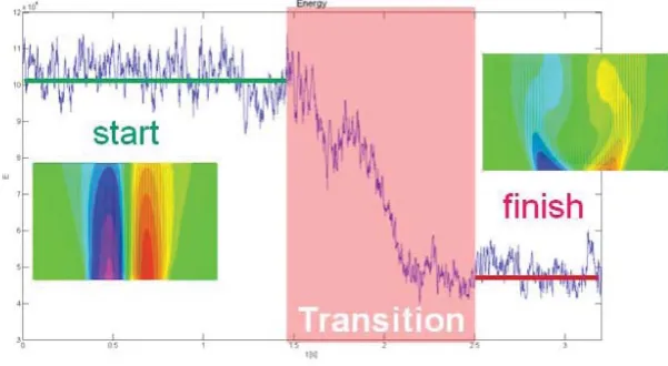
As the example of application of the BOD method on non-stationary data we will show results from the decay process of a swirling jet from [29].

The situation is characterized in Fig. 4, where total instantaneous energy of the system during the transition process from high-energy compact jet state (“start”) to low-energy jet decay state (“finish”) is seen. The transition between the states is covered by pink color.

Figure 4: Swirling jet decay – total energy time development

x [mm]

y [

mm]

Topos4

-60 -40 -20 0 20 40 60 -40

-30 -20 -10 0 10 20 30

-0.04 -0.03 -0.02 -0.01 0 0.01 0.02 0.03 0.04

transient, breakdown), the remaining modes are qualitatively state independent. The state-sensitive modes contain about 89% of the total kinetic energy; among them shift and oscillation modes are identified. Modes 1 to 3 exhibit strong changes during the transient state and more or less constant levels at the stationary states (before/after transient). In Fig. 5 the first mode – topos and chromos are shown, energy content is 75 % of the total energy. The mode 2 shows the similar structure as the mode 1.

Figure 5: The 1sttopos and chromos – a typical shift mode

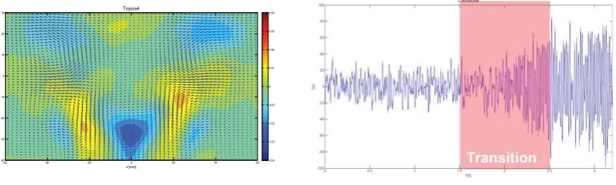
The 4thand 5thmode span the basis for an oscillating mode, as they both show an

oscillating signal, with the same amplitude and 1/4 period phase shift. They exhibit chaotic low intensity fluctuation during the first state and quasi-periodical behavior in the final state - see Fig. 6. These oscillation modes are related to the precision of vortex

breakdown. The energy of 4thmode is no more than about 0.8 % of the total energy.

Figure 6: The 4thtopos and chromos – a typical periodic mode

The typical random modes are characterized by small-grain structures in space distributed more or less uniformly. The chromos is typically random and stationary in statistical sense. There is no qualitative change of the mode during the transition

process. As an example see the 500th mode in Fig. 7 covering no more then 1.4 10-5 of

the total kinetic energy.

Figure 7: The 500thtopos and chromos – a typical random mode

5. S

TATISTICAL

(I

N

)D

EPENDENCE

Individual sources of perturbations in turbulent field could be assigned to independent time signals detected within the flow-field. Although the POD modes are orthogonal and thus uncorrelated, they are not necessarily independent. To decompose the turbulent signals into independent components some other method should be used. We suggest application of Independent Component Analysis (ICA) method. The ICA has been introduced in 80‘s to treat some neurophysiological problems (muscle contraction), while from 90’s it is applied in numerous fields of mathematics and physics. ICA is a statistical method, its goal is decomposition of a given multivariate data into a sum of statistically independent components. The method works with little prior information.

The Proper Orthogonal Decomposition extracts small number of the orthogonal components explaining maximal amount of variance possible. Both POD and ICA are linear transforms of multivariate data with aim of data compression and/or classification. The POD is based on second order statistics (correlations), it is orthogonal and provides optimal coding in least mean square sense, i.e. it maximizes variance content in the components.

The ICA is represented by the higher-order statistics and is related to projection pursuit. It is non-orthogonal transformation.

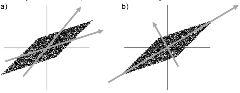
To compare both approaches let us consider the mixed components. The components evaluated using the ICA and POD procedures are shown in Fig. 8.

Figure 8: The mixed data decomposition using ICA (a) and POD (b)

The ICA finds the independent components (aka factors, latent variables or sources) by maximizing the statistical independence of the estimated components. We may choose one of many ways to define independence, and this choice governs the form of the ICA algorithms. The two broadest definitions of independence for ICA are minimization of mutual information and maximization of non-Gaussianity.

The Non-Gaussianity family of ICA algorithms, motivated by the central limit theorem, uses kurtosis and negentropy. The Minimization of Mutual Information family of ICA algorithms uses measures like Kullback-Leibler Divergence and Maximum-Entropy.

Let us define the statistical latent variables model first. We observe

n

linear mixtures

1

,...,

n

x

x

of

m

signals

s

₁

,...

s

_m:

1 1 2 2

...

j j j jm m

x

a s

a s

a s

,

j

1,...

n

(19) Note, that number of signals and mixtures could be different in general, there are no

restrictions even for theirs relation, i.e. the

n

could be equal, larger or even smaller then

m

. All mixtures and independent components are random variables

The starting point for ICA is the very simple assumption that the components

s

_i are

statistically independent. In addition we also assume that the independent components must have Non-Gaussian distributions, however we do not assume these distributions

known. Then, after estimating the matrix

A

, we can compute its inverse and obtain the

independent components. In tensor notation we have vectors

x

,

s

and matrix

A

:

˜

x A s

,

_{s A x}

1

_˜

₍₂₀₎

ICA is very closely related to the method called Blind Source Separation or Blind Signal Separation (BSS). “Blind” means that we know very little, if anything, on the mixing matrix, and make little assumptions on the source signals. ICA is one of the methods, perhaps the most widely used, for performing blind source separation.

Typical algorithms for ICA use centering, whitening (usually with the eigenvalue decomposition), and dimensionality reduction as preprocessing steps in order to simplify and reduce the complexity of the problem for the actual iterative algorithm. Whitening and dimension reduction can be achieved with POD or similar method. Whitening ensures that all dimensions are treated equally a priori before the algorithm is run.

However there are some ambiguities connected with the ICA method. In general, ICA cannot identify the actual number of source signals, a uniquely correct ordering of the source signals, nor the proper scaling (including sign) of the source signals. It could not indicate the components variances as well, because it introduces components normalization.

Uruba [28] has used the ICA method to construct independent modes of the dynamical system represented by reduced order POD model. The independent modes are linear combination of the POD modes, but they are considerably different.

6. S

TABILITY

M

ETHODS

Each stability mode is characterized by a complex frequency involving information on frequency, phase and growth/decay. There are several modifications of the method involving complex or cyclostationary variants.

6.1. P

RINCIPAL

O

SCILLATION

P

ATTERNS

In general the Principal Oscillation Patterns (POPs) method is very effective for studying travelling waves, on the other hand, this is unable to resolve standing oscillations.

The basis of the POPs analysis was formulated by Hasselmann [2] for discrete Markov processes in linearized dynamical systems driven by white noise with application in climatology. The POPs theory is a special case of more general Principal Interaction Patterns (PIPs) method for nonlinear dynamical systems.

In the POPs approach the fluctuating part of Navier-Stokes equation is modeled by Langevin equation for the linear Markov process:

d

t

t

t

dt

˜

u

B u

ȟ

,

(21)

where

u

t

is vector of velocity fluctuations, B is the deterministic feedback matrix,

t

ȟ

is noise driving the system which could be interpreted as influence of smaller,

unresolved scales. The equation (21) is a starting point for both POP and DMD methods,

however the way of the evaluation of eigenmodes of the operator B differs for the two

methods. Details on the DMD method see [18].

The noise

ȟ

t

in equation (21) forms covariance matrix

Q

, while the process itself is

characterized by the covariance matrix ȁ:

;

T T

ȁ

XX

4

ȟȟ

(22)

The Langevin equation (21) is a stochastic differential equation, which could be

transformed into a Fokker-Planck equation (see [3]). It could be rewritten for time lag

W

as followed:

t

W

W

˜

t

t

,

W

u

ȗ

G

u

, (23)

where

G

is the Green function.

1

exp

T

.

t

t

W

W

W

G

ȁ

B

u

u

(24)

The eigenvalues

g

_k of the Green function

G

are related to eigenvalues

E

_k of the

feedback matrix B as follows:

exp

k k

g

{

E W

. (25)

The real part of eigenvalues

E

_k characterizes the decay e-fold time

W

_ek of the POP (more

precisely its reciprocal value), this could be interpreted as the decay rate of our ability to predict development of the POPs. This must be negative for stable system. The imaginary part gives the

k

-th POPs oscillation frequency

f

_k:

Im

1

_;

Re

2

k

ek k

k

f

E

W

E

S

.

(26)

The noise matrix

Q

could be evaluated from the Fokker-Planck equation as well:

T

The POPs modes are the eigenfunctions of the matrix

G

and thus they are the empirically computed eigenmodes of the system.

Common eigenvectors form the set of POPs or normal modes. The right eigenvectors

v

_rk

of the

G

are computed as well as the left eigenvectors

v

_lk ofthe

_G

T_{. The left eigenvectors}

are called adjointor associated patterns very often – see e.g. [33]. The eigenvectors

could be reorganized into modal matrices

v

_r and

v

_land could be normalized in following

manner:

T T r l l r

v v

v v

I

,

(28)

whereI is the identity matrix. The diagonal eigenvalue matrix

ȕ

could be constructed as

well.

Then, the deterministic feedback matrix Band the Green function

G

could be formed:

;

T T

r l r

e

l W

W

ȕ

B v

ȕY

*

Y

Y

. (29)

Note that B and

G

matrices are obtained solely from the time series data

u

t

. If the

system is well described by a linear Markov process, then our estimate of

G

will be

independent of the choice of

W

. On the other hand, if nonlinear effects are important,

then

G

will vary significantly with

W

. As long as the linear approach holds, the

knowledge of the Green function could be used for a short-time forecasting of the system behavior using the equation (23) and neglecting the noise.

The matrix

G

is real non-symmetrical, so eigenvalues

E

and corresponding

eigenvectors

v

are complex and the complex conjugate

E

,

v

satisfy the eigenequation

as well. The complex eigenvectors

v

are defined only to within arbitrary complex

normalizationfactors. The modulus of the normalization factors can be specifiedby requiring, as usual, that

*

_,

₁

v v

.

(30)

This stillleaves the phase of the normalization factor free.A natural choice of phase angle in the complex plane is torequire that the real and imaginary components of the complexpattern, respectively, are orthogonal:

r

_{v v}

,

i

0

_.

(31)

In most cases, all eigenvalues are different and the eigenvectors form a linear basis. So

each state

u

t

may be uniquely expressed in terms of the eigenvectors

k k k

t

¦

z

u

v

. (32)

The coefficients of the pairs of conjugate complex eigenvectors are conjugate complex, too. Inserting (32) into (23) we find that the coupled system (23) becomes uncoupled,

yielding

n

single equations, where

n

is the dimension of the process

u

t

1

z t

˜ ˜

v

E

z t

˜

v

, (33)

so that if

z

0

1

than

t

z t

˜ ˜

v

O

v

. (34)

Then, contribution

V

t

of the complex conjugate pair

v

,

v

to the process

u

t

forms

t

z t

˜

ª

_¬

z t

˜

º

_¼

V

v

v

. (35)

The complex quantities could be written as follows

,

2

.

r i

r i

i

z t

z t

z t

i

˜

˜

v

v

v

(36)

The contribution is

cos

sin

r r i i t r i

t

z t

˜

z t

˜

U

˜

ª

_¬

K

t

˜

K

t

˜

º

_¼

V

v

v

v

v

, (37)

where

E U

˜

exp

i

K

for

z

0

1

. The geometric and physical meaning of (37) is that

between the spatial patterns r

v

and i

v

the trajectory

V

t

performs a spiral (Fig. 9)

with period

T

2

S K

and e-folding time

W

1 ln

U

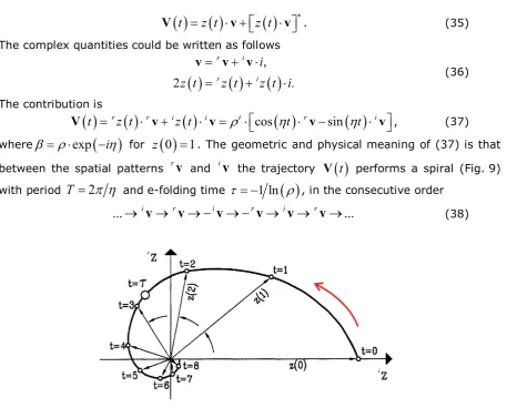
, in the consecutive order

...

_{o o}

i

_v

r

_v

_{o o o o}

i

_v

r

_v

i

_v

r

_v

_o

...

(38)

Figure 9: Time evolution of the POP signal

In Fig. 9 typical evolution the POPs signal is shown for r

z

0

0

andi

z

0

1

. In this

demonstration (from [17]) the period is

T

|

9

and the e-folding time is

W

|

2,8

.

The pattern coefficients

z t

are given as the dot product of

u

and adjoin patterns

v

A_j ,

which are normalized eigenvectors of the matrix

B

T:

T T

A A

j j k j k

k

z

v

u

¦

z

v

v

. (39)

To reduce the number of spatial degrees of freedom in some applications, the data are subjected to a truncated POD expansion, and the POPs analysis is applied to the vector of the first POD coefficients. A positive by-product of this procedure is that noisy components can be excluded from the analysis. Then, the covariance matrix has a diagonal form.

6.2. P

HYSICAL

I

NTERPRETATION OF

S

TABILITY

M

ETHODS

R

ESULTS

The eigenvalue characterizing each mode defines frequency and e-folding time. The frequency has obvious physical meaning. The e-folding time has to be considered with some caution, as noted by von Storch [33]. It represents formally the average time for

an amplitude of strength 1 to reduce to

1

e

. But in the POPs context this time is a

statistic of the entire time interval, it means that it is derived not only from the episodes when the signal is active but also from those times when the signal is weak or even absent. As such, the mode will be dampened less quickly as indicated by the e-folding time when the mode is active. The other limitation refers to the presence or absence of high-frequency variations. If these are filtered out, the e-folding time is lengthened.

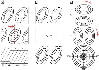
Each spatial pattern stability mode POP could be observed in the snapshots series, however it could be hidden in other modes occurring simultaneously. In Fig. 10 the 3 possible spatial modes are depicted schematically. The imaginary and real parts of a POP

are denoted as P1 and P2 respectively.

Figure 10: 3 types of spatial POP modes

In Fig. 10 the upper two rows show the representation in terms of real and imaginary

parts P1 and P2. Bottom row shows representation by phases (dashed curve) and

amplitudes (solid curve).

The 3 types correspond to (a) a linearly propagating wave, (b) a standing wave, and (c) a purely rotary wave.

The POPs in Figs. 10 (a) and 10 (c) have the amplitudes shown only if they are generated by a uniform phase forcing function. The amplitude distribution in Fig. 10 (c) has minima at the origin and outside the outer circle. The maximum is shown by the light curve. The red arrows indicate the structures movement.

In Figs. 10 (a)the structures propagation rate

U

_p could be calculated from a structure

displacement

s

during the half-period

T

2

or a mode frequency

f

:

2

₂

p

s

U

sf

T

.

(40)

The standing wave case in Fig. 10 (b) corresponds to uniformly decaying non-oscillating mode, because corresponding eigenvalue is real and thus the mode frequency is 0.

The rotation frequency in Fig. 10 (c) is given by mode frequency, of course.

However, distinguishing oscillatory and non-oscillatory modes in practical cases is not straightforward (although the pure real modes are possible). The oscillation of rapidly decaying modes is not very explicit. We could define really oscillating modes for example as those with decaying amplitude by one order (10-times) during one oscillating period.

That means that the ratio

n

of e-fold time

W

_e and oscillating period

T

1

f

should be

bigger than 0.43.

e e

n

f

T

W

_W

_.

(41)

The modes with smaller

n

could be termed pseudoperiodical or nearlyaperiodically

decayingmodes.

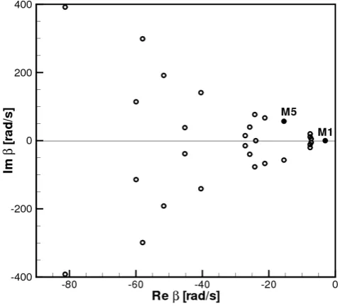
As an example we will present the case of dynamics of a boundary layer separation

presented in details in [25]. In Fig. 11 we see the

E

spectrum of 25 lowest POPs modes.

Figure 11: The POP spectrum

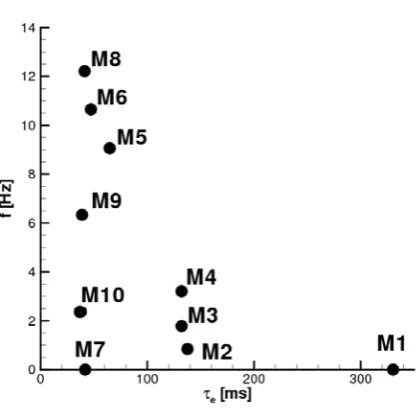
Figure 12: The first 10 modes – frequenciesand e-folding times

The mode 1 is aperiodic with e-fold time 330 ms, imaginary part of the modevanishes, real part is represented by vortical structures over whole separation region,see Fig. 13.

Figure 13: The 1stPOPs

The line represents location of zero mean longitudinal velocity component (the neutral line), arrows are velocity fluctuation vectors and color represents vorticity (red – positive, blue – negative).

The mode 2 is nearly aperiodic with the e-fold time about138 ms and period about 1.2 s

resulting in the ratio

n

0.12

, meaning that during one period the amplitude decays

down to 0.02 % of initial value. The mode 2 is in Fig. 14.

Figure 14: The 2ndPOPs

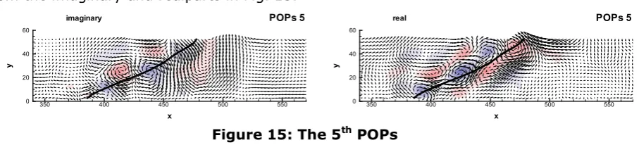
The first really oscillating mode is the mode 5 with e-fold time 65 ms and frequency

9.1 Hz. The resulting

n

0.59

means the decay ratio of 0.18 during the first period. The

x

y

350 400 450 500 550

0 20 40 60

POPs 1 imaginary

x

y

350 400 450 500 550

0 20 40 60

POPs 1 real

x

y

350 400 450 500 550

0 20 40 60

POPs 2 imaginary

x

y

350 400 450 500 550

0 20 40 60

mode represents system of vortexpairs travelling along the neutralline, this could be seen from the imaginary and realparts in Fig. 15.

Figure 15: The 5th POPs

7. C

ONCLUSIONS

The energetic methods rely on energetic contents of the modes, which are decorrelated. Unfortunately decorrelation does not mean necessarily independence of the modes. In reality the structures are not independent and they could be deterministic (e.g. periodical). The energetic modes are pulsating by definition. They are able to represent only Eulerian structures correctly, however the typical structures are Lagrangian, they are convected by the mean stream.

The stability approach offers more physical definition of structures entrained by mean flow and forming waves. The traveling modes are characterized by periodical topology with decaying amplitude and oscillation period. Those modes are really present in flow and could interact with the flow-field and the boundaries. Moreover, the sufficient set of the modes could be used for to build the model of the dynamical system, it could be used for a short-time forecasting.

8. A

CKNOWLEDGEMENTS

This work was supported by the Grant Agency of the Czech Republic, projects Nos. 101/08/1112 and P101/10/1230.

9. R

EFERENCES

[1] Adrian, R.J., Christensen, K.T., and Liu, Z.C., Analysis and interpretation of

instantaneous turbulent velocity fields, Experiments in Fluids, Vol. 29, No. 3,

2000, pp.275–290.

[2] Akhtar, I.,Nayfeh, A.H.,Ribbens, C.J., On the stability and extension of

reduced-order Galerkin models in incompressible flows. A numerical study of vortex

shedding,Theor. Comput. Fluid Dyn.(2009) 23,pp.213–237.

[3] Arnold, L., Stochastic Differential Equations: Theory and Applications. Wiley &

Sons, 1974, 228 pp.

[4] Aubry, N., Guyonnet, R., Lima, R., Spatiotemporal Analysis of Complex Signals:

Theory and Applications, Journal of Statistical Physics, vol.64, Nos.2/3, 1991,

pp.683-739.

[5] Cazemier, W., Proper Orthogonal Decomposition and Low Dimensional Models

for Turbulent Flows, PhD thesis, 1997, Rijksuniversiteit Groningen.

[6] Chang, C., Ding, Z., Yau, S.F. & Chan, F.H.Y., A Matrix-Pencil Approach to Blind

Source Separation of Colored Nonstationary Signals, IEEE Transaction on Signal

Processing, vol. 48, No. 3, 2000, pp. 900-907.

x

y

350 400 450 500 550

0 20 40 60

POPs 5 imaginary

x

y

350 400 450 500 550

0 20 40 60

[7] Garcia, A., Penland, C., Fluctuating Hydrodynamics and Principal Oscillation

Pattern Analysis, Journal of Statistical Physics, Vol.64, Nos.5-6, 1991,

pp.1121-1132.

[8] Gallagher, F., von Storch, H., Schnur R., Hannoschöck, G., The POP Manual

(POPs = Principal Oscillation Patterns), Modellberatungsgruppe, Hamburg, 1991.

[9] Hasselmann, K., PIPs and POPs: The Reduction of Complex Dynamical Systems

Using Principal Interaction and Oscillation Patterns. Journal of Geophysical

Research, 93, D9, 11.015-11.021, 1988.

[10] Hemon, P., Santi, F., Applications of biorthogonal decompositions in fluid–

structure interactions, Journal of Fluids and Structures17, 2003, pp.1123–1143.

[11] Hyvarinen, A. &Oja, E., Independent Component Analysis: Algorithms and

Applications, Neural Networks, vol. 13, No. 4-5, 2000, pp. 411-430.

[12] Hyvarinen, A., Karhunen, J. &Oja, E., Independent Component Analysis, John Wiley & Sons, 2001.

[13] Lumley J.L., The structure of inhomogeneous turbulent flows, Atm.Turb. and Radio Wave Prop., Yaglom and Tatarsky eds.,Nauka, Moskva, 1967,pp.166-178. [14] Lumley, J.L., Coherent structures in turbulence, Transition and Turbulence, (Ed.

R.E.Meyer), Academic Press, New York, 1981, pp.215-242.

[15] Penland, C., Random Forcing and Forecasting Using Principal Oscillation Pattern

Analysis, Monthly Weather Review, Vol.117, October 1989, pp.2165-2185.

[16] Sirovich L.: Turbulence and the dynamics of coherent structures. Quart. Appl.

Math., 45, 1987, pp.561-590.

[17] Springer Handbook of Experimental Fluid Mechanics, (Eds.: Tropea C., Yarin A.L., Foss J.F.), 2007.

[18] Schmid, P.J., Dynamic mode decomposition of numerical and experimental data,

J. Fluid Mech.(2010), vol. 656, pp.5–28.

[19] Tropea, C., Yarin, A.L., Foss, J.F. eds.: Handbook of Experimental Fluid Mechanics, 2007, Springer.

[20] Uruba, V., Knob, M., Popelka, L., Dynamics of a synthetic jet, Colloquium Fluid

Dynamics 2006, Proceedings, Praha, Institute of Thermomechanics AS CR,

(Eds.: Jonáš, P., Uruba, V.), 2006, pp.137-140.

[21] Uruba, V., Knob, M., Dynamics of Controlled Boundary Layer Separation, Colloquium Fluid Dynamics 2007

Uruba V.), pp.95-96.

[22] Uruba, V., Knob, M., Spatiotemporal Analysis of a Synthetic Jet Flow-Field,

Conference Topical Problems of Fluid Mechanics 2007

!"#$*"+<<>?Q-188. (b)

[23] Uruba, V., Boundary Layer Separation Dynamics, Conference Topical Problems

of Fluid Mechanics 2008 !"#$*

K.), pp.125-128.

[24] Uruba, V., Knob, M., Application of the Orthogonal Decomposition Methods,

22nd Symposium on Anemometry, national conference with international

participation, (Eds.: Chára, Z.; Klaboch, L.), Holany-Litice, June 2008, Proceedings, pp.103-108.

[25] Uruba, V., Boundary Layer Separation Dynamics, In: Conference Topical

Problems of Fluid Mechanics 2008 ! ""#$*

[26] Uruba, V., Methods of Dynamical Analysis of Spatio-Temporal Data, 23th

Symposium on Anemometry, (Eds.: Chára, Z.; Klaboch, L.) Institute of

Hydrodynamics ASVR, v. v. i., 2009, pp.110-115.

[27] Uruba, V., Dynamics of a Boundary Layer Separation. In: 14th CMFF 09,

University of Technology and Economics, Budapest, (Ed.:Vad, J.), 2009,

pp.268-275.

[28] Uruba, V., Independent Component Analysis for Identification of Coherent

Structures, In: 24th Symposium on Anemometry (Z.Chára&L.Klaboch eds.),

2010, pp.118-123.

[29] Uruba, V.,Oberleithner, K.,Sieber, M.,Hladík, O., SPATIO-TEMPORAL ANALYSIS

OF SWIRLING JET UNSTEADY BREAKDOWN. In Colloquium Fluid Dynamics

2010: Proceedings. Prague : Institute of Thermomechanics AS CR, v. v. i.,

2010. pp.29-30.

[30] Uruba, V., Independent modes in a boundary layer separation region,17th

International Conference ENGINEERING MECHANICS 2011,Svratka, Czech

Republic, 9 – 12 May 2011, pp.631-634.

[31] von Storch, H., Bruns, T., Fischer-Bruns, I., Hasselmann, K., Principal Oscillation Pattern Analysis of the 30- to 60-Day Oscillation in General Circulation Model

Equiatorial Troposphere, Journal of Geophysical Research, Vol.93, No. D9, 1988,

pp.11.022-11.036.

[32] von Storch, H., Xu, J., Principal Oscillation Pattern analysis of the 30- to 60-day

oscillation in the tropical troposphere, Climate Dynamics (1990) vol.4,

pp.175-190.

[33] vonStorch, H., Burger, G., Schnur, R., von Storch, J.-S., Principal Oscillation