Can compact optimisation algorithms be
structurally biased?
Anna V. Kononova1[0000−0002−4138−7024], Fabio Caraffini2[0000−0001−9199−7368], Hao Wang3[0000−0002−4933−5181], and Thomas B¨ack1[0000−0001−6768−1478]
1 Leiden Institute of Advanced Computer Science (LIACS), Leiden University, The Netherlands
{a.kononova,t.h.w.baeck}@liacs.leidenuniv.nl 2
Institute of Artificial Intelligence, De Montfort University, UK [email protected]
3
LIP6, Sorbonne Universit´e Paris, France [email protected]
Abstract. In the field of stochastic optimisation, the so-called
struc-tural bias constitutes an undesired behaviour of an algorithm that is
unable to explore the search space to a uniform extent. In this paper, we investigate whether algorithms from a subclass ofestimation of
distri-bution algorithms, the compact algorithms, exhibit structural bias. Our
approach, justified in our earlier publications, is based on conducting experiments on a test function whose values are uniformly distributed in its domain. For the experiment, 81 combinations of compact algorithms and strategies of dealing with infeasible solutions have been selected as test cases. We have applied two approaches for determining the pres-ence and severity of structural bias, namely a visual and a statistical (Anderson-Darling) tests. Our results suggest that compact algorithms are more immune to structural bias than their counterparts maintaining explicit populations. Both tests indicate that strong structural bias is found only in one of the algorithms (cBFO) regardless of the choice of strategy of dealing with infeasible solutions andcPSO mirror. For other test cases, statistical and visual tests disagree on some cases classified as having mild or strong structural bias: the former one tends to make harsher decisions, thus needing further investigation.
Keywords: structural bias·compact algorithm·continuous optimisa-tion·estimation of distribution algorithm·infeasible solution.
1
Introduction
Evolutionary algorithms (EAs) [8, 1] are based on a biological metaphor which creates an ontological link between a set of solutions of the optimisation prob-lem, which iteratively approximate its optimum, and a population of biological individuals, which adapt to their environment through evolution. An essential part of this metaphor is an individual, an atomic part of the population, that has been created by some combination of one or more of its parent individuals
in an attempt to build upon previously successful approximations of the opti-mum. Both biological and (most) computational populations typically do not explicitly ‘record’ their history, thus, potentially loosing the already exploited information regarding the ‘successes’ in the past generations. Following the bi-ological metaphor, a ‘success’ in some generation is directly translated into the individual’s reproductive advantage and, therefore, an opportunity to pass on its ‘achievements’.
Striving to exploit the historical information contained in the sequential pop-ulations of an evolutionary algorithm, a special class of algorithms has been been proposed in the 1990s [17, 16] which attempts to buildexplicit probabilistic
mod-els of promising solutions as the optimisation process progresses and steer the
subsequent simulated evolutionary progress towards such solutions. These new algorithms, just like other heuristics [14, 18, 6], are probabilistic, iterative, and thus can suffer from undesirable algorithmic behaviours such as premature con-vergence, stagnation and presence of structural bias (SB) [14, 6]. The latter is
thefocus of this paper.
The aforementioned class of algorithms, referred to asestimation of
distri-bution algorithms (EDAs) [9], do not maintain explicit populations but rather
havevirtual sampling populations. They work through updating their models
in-crementally, starting from some uninformed prior and, ideally, leading up to the model producing only the optimum solution. Clearly, the problem of construct-ing such a model in itself is by far not trivial and can only be solved with some simplifications. It is the scope and extent of suchsimplifications that define the sub-classes of EDAs.
This paper addresses the question of whether asubclass of algorithms with virtual populations exhibit such algorithmic deficiency as structural bias – the tendency of an algorithm to ‘prefer’ some parts of the domain irrespective of the objective function. The paper is organised as follows: Section 2 discusses compact algorithms in general and the particular instances investigated in this study, Section 3 describes the experimental methodology and methods for assessing SB, Section 4 discusses results concerning SB in compact algorithms, and Section 5 provides the conclusions.
2
Compact algorithms
The term ‘compact algorithm’ refers to those EDAs mimicking the behaviour of established population-based algorithms [10] through a ‘memory-saving’ prob-abilistic model where design variables are assumed to be uncorrelated. This minimalist model is fully described with a 2×n matrix (n is problem di-mensionality) that defines the generating distribution4 D
θ, where θ = [µ,σ],
dard deviation values for a truncated Gaussian distribution (the optimisation process takes places in there-normalised domain [−1,1]n).
All ‘elitist’ real-valued compact algorithms share the structure outlined in Algorithm 1 and only differ by the logic used to generate a new solutionx.
Algorithm 1Skeleton of a generic elitist compact algorithm
given:objective functionf, generating distributionDθ with parametersθ= [µ,σ]
initialiseµ,σ withµi= 0 andσi1 .e.g.σi= 10 as in [10]
draw initial solutionxelitefromDθ and evaluate its fitnessfelite=f(xelite) whilebudget condition is not metdo
draw i.i.d. samplesP={x1,x2, . . .}fromDθ .|P|depends on the specific
generate a new candidate solutionxfromP operator (Section 2.1) evaluatef(x);
if f(x)./ felite then . ./∈ {≤,≥}for minimisation/maximisation l←xelite;w←x;xelite←x; .wis the winner,lloser else
l←x;w←xelite; end if
µold←µ
µ←µ+ 1
Vps(w−l) .user defined virtual population sizeVps[10] σ←qσ◦σ+µold◦µold−µ◦µ+
1
Vps(w◦w−l◦l)
end while .◦is the Hadamard product
Output:xelite
2.1 Compact algorithms employed in this study
Details on the employed algorithms, including their suggested and adopted pa-rameters setting, are available in [10]. A brief description of each algorithm is given below. These algorithms are equipped with various strategies of dealing with infeasible solutions (SDIS) generated, see Section 3.4.
Configurable compact differential evolution(cDE/x/y/z): similar to non-compact variants of differential evolution [19], a variety of non-compact configu-rations can be obtained with the combinations x/y/z, where z is either the binary bin or the exponential exp crossover [5, 19], while the x/ycomponent is taken from these options5: (i)
rand/1 (ii) rand/2 (iii) best/1 (iv) best/2 (v) current-to-best/1 (vi) rand-to-best/2 (vii) current-to-rand/1 (does not require a crossover). It must be highlighted that in a DE algorithm, thex/y/z operators require a number of randomly selected individuals from the population to producex. Due to the absence of a stored population, these individuals are drawn from the generating distributionDθ in the compact representation. This implies that logicallycurrent-to-best/1≡rand-to-best/1.
Compact differential evolution light:cDE-Lightis a DE-inspired compact algorithm that requires a smaller number of computationally expensive opera-tions with respect to its predecessor algorithmcDE, thus being faster and lighter
5
in terms of memory consumption. This algorithm employs a specific mutation referred to asmutation-light, which mimics the behaviour of therand/1 mu-tation, and specific crossover operator referred to as crossover-light, which emulates theexpcrossover without the need of looping through the solutions to exchange their variables.
Compact particle swarm optimisation (cPSO): generates novel candidate solutionsxthrough the simplePSOperturbation logic based on a weighted sum of the currently available solution and the so-called ‘velocity’ vectorv, i.e.x← γ1x+γ2v. Before perturbing the position of x in the search space with the previous formula, the v is updated through the following minor alteration of the standard methodv←φ1v+φ2u1◦(xlb−x) +φ3u2◦(xgb−x), in which
u1 and u2 are two n-dimensional vectors containing uniformly drawn random
numbers; xlb is the ‘local best’ solution, which is not present in the compact
representation and therefore has to be drawn from Dθ and evaluated; xgb is
the ‘global best’ solution, i.e., xgb ←xelite. It must be pointed out thatDθ is updated withw andlobtained by comparing the objective function valuesxlb
andxwhile thexelite solution is subsequently updated.
Compact bacterial foraging optimisation(cBFO) reproduces the same search logic of the original BFO algorithm [7] with the difference that, at each iteration, a candidate solutionxis drawn fromDθrather than being taken from a popula-tion. Such solution undergoes a series of perturbations to perform the so called ‘chemotaxis’, ‘tumble’ and ‘swim’ moves in the search space by means of the operatorx←x+√c◦∆
∆T∆, wherecis ann-dimensional vector whose components
are the so-called ‘run-length’ unit parameters [7], which control the step-size, and ∆is an n-dimensional vector whose components are uniformly sampled in the interval [−1,1] as indicated in [7] for each one of the three moves.
Compact genetic algorithm: the real-valued compact genetic algorithmrcGA [10], orcGAhere, is the simplest example of compact algorithm as it only draws a new solution fromDθ(i.e.P ={x}) to produce a new candidate solution.
3
Methodology
3.1 Structural bias
In the EA/EC community, variations of the first two of the aforementioned dimensions are traditionally used. However, most performance measures come with a difficulty: dependence on the objective function [21]. Moreover, in practice, classes of objective functions are typically hard to be defined exhaustively and extensively and benchmarking over a set of diverse functions strongly depends on the choice of such functions.
In an attempt to characterise the performance of optimisation algorithms
from a different angle, an additional fitness-free comparison ‘dimension’ has
been suggested in [14]: the so-called structural bias (SB) has been defined as
an intrinsic deficiency of a probabilistic iterative algorithm dictated solely by
its structure. An algorithm is said to possess SB when it is unable to explore all areas of the search space to a uniform extent, irrespective of the objective function.
In other words, characterising the algorithm in terms of SB allows one to judge how muchgeneral-purpose the algorithm is, since a fully general-purpose optimisation algorithm is expected to be able to locate the optima regardless of where they are located in the search space. It has been established [14] that for a general objective function, the movement of solutions in the populations evolving over time is dictated by the superposition of two forces: the gradient formed by the values of objective function in the current population and the force originating from the structure of algorithm. Thesetwo forces are not necessarily
in agreement in terms of direction and strength. The problem with the existence
of the second force is that it can potentially pull the search away from some areas of the domain, thus limiting the algorithm’s ability to find the optima herein.
It must be remarked that due to the stochastic nature of the utilised test function f0 (see Section 3.2), there is no sense in tracking objective function improvements over time. The goal of tests onf0 isonly to establish deficiencies in movements of the populations during the optimisation process andnot to rank
the methods according to their ‘objective-function-improvement’ onf0.
3.2 Structural bias via visual tests
The procedure for testing for presence of SB is based on atheoretical result [14]
that true minima/maxima of f0 : [0,1]n →[0,1] where ∀x f0(x)∼ U(0,1) are
distributed uniformly in its domain. Thus, through examination of the
distribu-tion of locadistribu-tions of the optima identified by the algorithm and its subsequent comparison to the true uniform distribution across the domain, one can establish whether the algorithm exhibits any SB [14].
To date, such comparison is done visually due to the lack of a good
‘all-encompassing’ measure, see Section 3.3 for more discussion. Plotting locations
3.3 Structural bias via statistical tests
To identify SB, we build on the previous studies [14, 13] where Kolmogorov-Smirnov test has been used for hypothesis testing. Here, we propose a different statistical approach whichtests the uniformityof final points per dimensionvia a
non-parametric goodness-of-fit test – the Anderson-Darling (AD) test is chosen
given its high statistical power [20]. The motivation behind this approach is two-fold: first, testing the multivariate uniformity is known to be achallenging
task [12]; second, it is methodologically erroneous to merge samples from all dimensions to perform one univariate good-of-fit test as the design variables could be correlated and not identically distributed, thus resulting in a potential loss of information on each dimension.
Hence, for each dimensioni∈[1..n] the AD test is applied to theith compo-nent of final points{x(1)i , . . . , x(Nr)
i }obtained overNrindependent runs (Nr= 50 here). When testing the uniformity of the sample distribution along each dimen-sion, the AD test-statistic is formulated as:A2=R1
0(FbNr(t)−t)
2/t(1−t)dt,where
b
FNr(t) =
PNr
k=11(x (k)
i ≤ t) is the empirical cumulative distribution function (ECDF) of theith component. Intuitively,A2quantifies the proximity between the ECDF and the theoretical distribution function of the uniform distribution. We shall denote the resulting test statistics andp-values as{A2
i}ni=1and{pi}ni=1 respectively. The significance levelα= 0.01 is used to reject the null hypotheses H0. WheneverH0 is rejected we conclude that the ECDF differs from the uni-form distribution by an amount ofA2, with an error rate ofα. The SB ‘degree’ is then determined by counting therejected dimensions.
Moreover, we propose an aggregated measure of SB over results from all dimensions, defined as the sum ofA2i test statistics that are associated with a statistical significance over all dimensions: SB = 1nPn
i=1A 2
i1(pi ≤α), where1 stands for the indicator function. We shall contrast this new measure of SB with the visual test shown in Section 4.2.
3.4 Strategy of dealing with infeasible solutions as operator
Practical optimisation problems to be solved via computer simulations are de-fined in a bounded domain whose most typical shape is hyperrectangular. Re-search into the algorithmic design of optimisation methods from the field of com-putational intelligence [6] has shown that the chosen strategy of dealing with the solutions generated outside such domain – theinfeasible solutions (ISs) – is an
essential part of the algorithm that to a large extent decides the success of the
optimisation method. Unfortunately, in the majority of papers in the field, the choice of such strategy is typically overlooked or omitted from the publications, thus limiting the reproducibility of the results and lowering the overall impact of such studies.
3.5 Experimental setup
This experimentation involves 13cDE/x/y/zvariants and the 4 other algorithms described in Section 3.4. All of them but cGA (which generates only feasible solutions) are considered with 5 SDIS – the total of 16×5+1 = 81 configurations considered.
Results on the SB presented in this paper are based onexperiments: (i)
min-imising the test functionf0 (see Section 3.2) forn= 30 (ii) by 81 algorithmic
configurations described in Sections 2.1 and 3.4; (iii) each configuration is run 50 times; (iv) each run has independently seededJava random.utils pseudorandom generator – seed is initialised with the current time since January 1, 1970 in milliseconds via Java’s System.currentTimeMillis; (v) each run is budgeted in terms of the number of objective function evaluations as 10000n.
All algorithms refer to their persistent elitist variants. All experiments are executed on a standard desktop using the SOS platform [3] implemented in Java (algorithms’ source code is available online). It is worth mentioning that the aforementioned pseudorandom generator used for all experiments is considered
on the better side of the scale for linear congruential generators [15]
4
Discussion of results
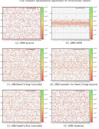
Using the approaches described in Sections 3.2 and 3.3, all 81 configurations have been investigated. Results in these figures are shown inparallel coordinates [11]
andshould be read as follows: final positions attained in a series of 50 independent
runs of each configuration are shown with 50 ‘+’ markers on each of the n = 30 parallel vertical ‘axes’. Positions of these ‘axes’ identify dimensions and are shown on the traditional horizontal axis; meanwhile, the traditional vertical axis shows the range of the dimension ([0,1] here). Values off0attained by the final solutions are shown in colour (a recap: this is a minimisation problem). Due to the page limit in this publication, only a few figures are shown in Fig. 1. All results can be obtained from [5].
4.1 Visual tests
Following the methodology of visual testing described in Section 3.2, out of 81 configurations considered in this paper, only 6 configurations have been found to be structurally biased (e.g. Figs. 1(a), 1(b)), meanwhile 40 configurations exhibit only mild SB. It is worth highlighting that decisions in visual tests on whether mild SB is present are highly subjective and should be contrasted with results from statistical testing in Section 4.2.
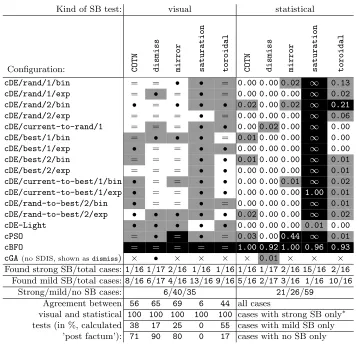
The summary of results discussed in this Section can be found in Table 1 in the columns marked as ‘visual SB test’ for all basic compact configurations (rows) and all strategies of dealing with IS (smaller columns)6.
6
Table 1.Comparison of results on the presence and strength of structural bias based
on visual and statistical tests across all 81 configurations (see [5]). For both tests,
cells with background inblack mark configurations exhibiting strong SB, ingrey -configurations with mild SB and inwhite- configuration with no SB identified based on the corresponding tests (i.e. colour marks the corresponding decision of the test). Cells containing ‘×’ mark configurations that are not possible by design.Symbols mark
results of comparing the two tests: symbol ‘=’ stands for cells where results of the
visual and statistical tests coincide (colour of the symbol has no meaning) and ‘•’ - for the differences in results from visual and statistical tests (colour of the symbol has no meaning). Values shown in columns for statistical test are thecorresponding values of
the statistic. Thresholds for decisions based on these values are given in Section 4.2.
Kind of SB test: visual statistical
Configuration: COTN dismiss mirror saturation toroidal COTN dismiss mirror saturation toroidal
cDE/rand/1/bin = = • • = 0.00 0.00 0.02 ∞ 0.13 cDE/rand/1/exp = • = • = 0.00 0.00 0.00 ∞ 0.02 cDE/rand/2/bin • = • • • 0.02 0.00 0.02 ∞ 0.21
cDE/rand/2/exp = = = • = 0.00 0.00 0.00 ∞ 0.06 cDE/current-to-rand/1 = = = • • 0.00 0.02 0.00 ∞ 0.00 cDE/best/1/bin = • • • = 0.01 0.00 0.00 ∞ 0.00 cDE/best/1/exp • = = • • 0.00 0.00 0.00 ∞ 0.00 cDE/best/2/bin = = = • • 0.01 0.00 0.00 ∞ 0.01 cDE/best/2/exp = = = • • 0.00 0.00 0.00 ∞ 0.01 cDE/current-to-best/1/bin • = = • • 0.00 0.00 0.01 ∞ 0.02 cDE/current-to-best/1/exp • = = • • 0.00 0.00 0.00 1.00 0.01 cDE/rand-to-best/2/bin • = = • = 0.00 0.00 0.00 ∞ 0.01 cDE/rand-to-best/2/exp • • • • • 0.02 0.00 0.00 ∞ 0.02 cDE-Light • • • • • 0.00 0.00 0.00 0.01 0.00
cPSO = • = • = 0.03 0.000.44 ∞ 0.01
cBFO = = = = = 1.00 0.92 1.00 0.96 0.93
cGA(no SDIS, shown asdismiss) × • × × × × 0.01 × × × Found strong SB/total cases:1/16 1/17 2/16 1/16 1/16 1/16 1/17 2/16 15/16 2/16
Found mild SB/total cases: 8/16 6/17 4/16 13/16 9/16 5/16 2/17 3/16 1/16 10/16 Strong/mild/no SB cases: 6/40/35 21/26/59
Agreement between 56 65 69 6 44 all cases
visual and statistical 100 100 100 100 100 cases with strong SB only∗ tests (in %, calculated 38 17 25 0 55 cases with mild SB only
0 0.2 0.4 0.6 0.8 1
1 2 3 4 5 6 7 8 9 10 11 12 13 14 15 16 17 18 19 20 21 22 23 24 25 26 27 28 29 30 finpos cPSOmD30f0 0 5x10⁻⁶ 1x10⁻⁵ 1.5x10⁻⁵ 2x10⁻⁵ 2.5x10⁻⁵ 3x10⁻⁵ 3.5x10⁻⁵
(a)cPSO mirror
0 0.2 0.4 0.6 0.8 1
1 2 3 4 5 6 7 8 9 10 11 12 13 14 15 16 17 18 19 20 21 22 23 24 25 26 27 28 29 30 finpos cBFOcD30f0 0 5x10⁻⁶ 1x10⁻⁵ 1.5x10⁻⁵ 2x10⁻⁵ 2.5x10⁻⁵ 3x10⁻⁵ 3.5x10⁻⁵
(b) cBFO COTN
0 0.2 0.4 0.6 0.8 1
1 2 3 4 5 6 7 8 9 10 11 12 13 14 15 16 17 18 19 20 21 22 23 24 25 26 27 28 29 30 finpos cDEboetD30f0 0 5x10⁻⁶ 1x10⁻⁵ 1.5x10⁻⁵ 2x10⁻⁵ 2.5x10⁻⁵ 3x10⁻⁵ 3.5x10⁻⁵
(c)cDE/best/1/exp toroidal 0 0.2 0.4 0.6 0.8 1
1 2 3 4 5 6 7 8 9 10 11 12 13 14 15 16 17 18 19 20 21 22 23 24 25 26 27 28 29 30 finpos cDEctboemD30f0 0 5x10⁻⁶ 1x10⁻⁵ 1.5x10⁻⁵ 2x10⁻⁵ 2.5x10⁻⁵ 3x10⁻⁵ 3.5x10⁻⁵
(d)cDE/current-to-best/1/exp mirror
0 0.2 0.4 0.6 0.8 1
1 2 3 4 5 6 7 8 9 10 11 12 13 14 15 16 17 18 19 20 21 22 23 24 25 26 27 28 29 30 finpos cDErobtD30f0 0 5x10⁻⁶ 1x10⁻⁵ 1.5x10⁻⁵ 2x10⁻⁵ 2.5x10⁻⁵ 3x10⁻⁵ 3.5x10⁻⁵
(e)cDE/rand/1/bin toroidal 0 0.2 0.4 0.6 0.8 1
1 2 3 4 5 6 7 8 9 10 11 12 13 14 15 16 17 18 19 20 21 22 23 24 25 26 27 28 29 30 finpos cPSOdD30f0 0 5x10⁻⁶ 1x10⁻⁵ 1.5x10⁻⁵ 2x10⁻⁵ 2.5x10⁻⁵ 3x10⁻⁵ 3.5x10⁻⁵
(f)cPSO dismiss
Fig. 1. Distribution of locations of final best solutions, example configurations that exhibitstrongSB in Figs. 1(a), 1(b),mild SB with:local clustering in Fig. 1(c),
clus-tering across domain in Fig. 1(d), clustering on boundaries domain in Fig. 1(e) and
large gaps in Fig. 1(f). See Section 4 for explanation on how to read this figure.
Based on the visual tests only, overall, compact configurations appear to
be more ‘immune’ to the strong SB than their equivalents maintaining explicit
and not in the span of the domain (with exception of all cBFO configurations as discussed below). It means that, on the whole, compact configurations of algorithms considered in this studyshould have more exploratory potential and be more successful in finding optima wherever they are situated in the domain. The latter one, however, isnot guaranteed without the use of good exploitative operators (such investigation is out of the scope of this paper).
One of the exceptions to the above statement is all thecBFOconfigurations that have turned out to be badly biased towards the middle of the domain regardless of the choice of correction strategy, e.g. Fig. 1(b). More precisely, cBFO appears to be unable to find optima on f0 outside the region [0.4,0.6]30 (with only a handful of exceptions per configuration).
Another exception to the above statement is thecPSO mirrorconfiguration which exhibits strong SB towards all corners of the domain (see Fig. 1(a)) –
interestingly enough, such situation resembles the case of non-compact PSOwith
a small population size [14].
When talking aboutmild SB, resulting distributions of the locations of final best solutions appear tomarginallydeviate from the uniform distribution in the following non-exclusive aspects:
1. ‘higher-than-expected’ clustering of pointswithinthe domain (e.g. Fig. 1(c)); 2. ‘higher-than-expected’ clustering of pointsacrossthe domain (e.g. Fig. 1(d); 3. ‘higher-than-expected’ clustering of points on theboundaries7(e.g. Fig. 1(e));
4. large empty gaps consistently identified in all 30 dimensions (e.g. Fig. 1(f)).
When analysing results forcDE/x/y/zonly, out of 30 binand 30exp con-sidered configurations, 16 and 13, respectively, appear to bemildly biased. Out 5 cDE/current-to-rand/1 configurations that require no crossover, 3 appear to be mildly biased. To some extent, it is fair to say that simpler cDE/x/y/z
configurations with y>1 appear to befreer of mild SB.
4.2 Statistical tests
Here, we present the calculated values of the statistical measure of structural bias (defined in Section 3.3) in the ‘statistical SB test’ column of Table 1 (the meaning of symbols and colour scales are explained in the table caption). We use the 20- (0.00) and 90-quantiles (0.158)8 of the statistical values over all combinations asthresholds to determine the level of SB. More specifically, zero values of statistic shall be classified as havingnoSB; ranges formild andstrong
SB are (0,0.158] and (0.158,1]∪ {+∞}, respectively.
From results presented in the table, it is obvious thatcBFO is exceptionally biased regardless of the SDIS. Also, thesaturationSDIS seems to yield strong SB for all the algorithms except cDE-Light. For the remaining combinations, we observe either no or mild SB.
7 This is easily explained if saturationis used but is not trivial if toroidalis used. 8
Comparing to the visual test on the same combinations, it seems that cases classified as strongly biased by the visual tests are always indicated as strongly biased as well from the statistical side – see the third line from the bottom in Table 1, marked with ∗. However, since there are at most two discoveries of the strong bias from both tests,the reliability of this agreement is questionable. In contrast, cases with mild SB in the visual test are largely mis-classified as possessing no SB in the statistical approach. Also, most of the algorithms with thesaturationSDIS are indicated as strongly biased by the statistical measure while those cases are considered mildly biased in the visual test. We conjecture the observed mismatches between those two approaches as follows: (i) the SB measure is calculated from a multiple testing procedure, where the p-value is corrected, thus the SB measure can suffer from a reduction of its statistical power (i.e., more false-negative decisions are made). This leads to a scenario that the Anderson-Darling test is rejected on all dimensions for those cases with mild SB in the visual test and hence the statistical measure classifies them as not biased; (ii) the SB measure is not scale-invariant and can be less informative after the performed normalisation. In this light, when no bias is displayed, we shall conclude that some SB degree is exhibited but negligible if compared to the bias shown by the most biased algorithm (i.e., cBFO). Such relativity in the statistical approach might be different from that in the visual test, which leads to the observed discrepancy.
5
Conclusions
The extensive experimentation presented in this piece of research has unveiled the presence of mild structural biases for most compact algorithms exceptcBFO, which carries a so strong SB that can be categorically detected by visual inspec-tion of the generated graphs. More precisely, incBFO, regardless of the employed SDISs, only the middle section of the search domain is populated by the best solutions, while its peripheral areas are left completely out. This undesired al-gorithmic behaviour suggests that cBFO is not suitable for general-purpose op-timisation, since displaying design flaws limiting its applicability to problems whose optimum/optima is/are at the centre of the search space. Similarly, also cPSO mirrordisplays a visible strong bias. However, it is interesting to observe that in this case, the solutions obtained over multiple runs accumulate towards the corners of the search space. This behaviour is in line with the one of the standard PSOalgorithm – when employed with a small population size [14].
SB is mainly visible only for those cases equipped with mutation operators using one difference vector – e.g. this is evident for thebest/1mutation, in particular when used in combination with binomial crossover bin.cDE variants equipped with mutation operators using two difference vectors, on the other hands, seem to be freer from SB – e.g. the case of rand/2, in particular when followed by exponential crossoverexp.
To summarise, it can be stated that the compact algorithms under investi-gations appeared to be more ‘immune’ to the SB than their population-based equivalents according to the proposed visual test. However, it is important to con-clude this study by observing that the proposed statistical SB detection method agrees with the visual test on strong SB cases while disagrees on most of the visually detected mild SB cases. We speculate that this discrepancy is caused by the insufficient sample size as well as the conservative nature of this testing procedure and we commit to investigating this aspect further in our future stud-ies. We plan to increase the sample-size in future experimentation and, most importantly, improve upon the sensitivity of the proposed statistical measure with respect to the number of independent runs.
References
1. B¨ack, T.: Evolutionary Algorithms in Theory and Practice. Oxford University Press, New York, NY (1996)
2. Campelo, F., Aranha, C.: EC Bestiary: A bestiary of evolutionary, swarm and other metaphor-based algorithms (Jun 2018). https://doi.org/10.5281/zenodo.1293352 3. Caraffini, F.: The SOS platform: designing, tuning and
statisti-cally benchmarking optimisation algorithms. MDPI Preprints (2020). https://doi.org/10.20944/preprints202003.0381.v1
4. Caraffini, F., Kononova, A.V.: Structural bias in differential evolution: a prelimi-nary study. In: LeGO 2018 - 14th International Workshop on Global Optimization. vol. 2070, p. 020005. AIP, Leiden, The Netherlands (2018)
5. Caraffini, F., Kononova, A.V.: Structural Bias in Optimisation Algorithms: Ex-tended Results (2020). https://doi.org/10.17632/zdh2phb3b4.2, mendeley Data 6. Caraffini, F., Kononova, A.V., Corne, D.W.: Infeasibility and structural
bias in differential evolution. Information Sciences 496, 161–179 (2019). https://doi.org/10.1016/j.ins.2019.05.019
7. Das, S., Biswas, A., Dasgupta, S., Abraham, A.: Bacterial Foraging Optimiza-tion Algorithm: Theoretical FoundaOptimiza-tions, Analysis, and ApplicaOptimiza-tions, pp. 23–55. Springer (2009). https://doi.org/10.1007/978-3-642-01085-9 2
8. De Jong, K.A.: An Analysis of the Behavior of a Class of Genetic Adaptive Systems. Ph.D. thesis, University of Michigan, USA (1975)
9. Hauschild, M., Pelikan, M.: An introduction and survey of estimation of distri-bution algorithms. Swarm and Evolutionary Computation1(3), 111–128 (2011). https://doi.org/10.1016/j.swevo.2011.08.003
11. Inselberg, A.: The plane with parallel coordinates. The Visual Computer 1(2), 69–91 (1985). https://doi.org/10.1007/BF01898350
12. Justel, A., Pe˜na, D., Zamar, R.: A multivariate Kolmogorov-Smirnov test of good-ness of fit. Statistics & Probability Letters35(3), 251–259 (1997)
13. Kononova, A.V., Caraffini, F., Wang, H., B¨ack, T.: Can single solu-tion optimisasolu-tion methods be structurally biased? MDPI Preprints (2020). https://doi.org/10.20944/preprints202002.0277.v1
14. Kononova, A.V., Corne, D.W., Wilde, P.D., Shneer, V., Caraffini, F.: Structural bias in population-based algorithms. Information Sciences 298, 468–490 (2015). https://doi.org/10.1016/j.ins.2014.11.035
15. L’Ecuyer, P., Simard, R.: TestU01: A C Library for Empirical Testing of Random Number Generators. ACM Transactions on Mathematical Software33(4) (2007). https://doi.org/10.1145/1268776.1268777
16. M¨uhlenbein, H., Paaß, G.: From recombination of genes to the estimation of distri-butions i. binary parameters. In: Voigt, H.M., Ebeling, W., Rechenberg, I., Schwe-fel, H.P. (eds.) Parallel Problem Solving from Nature – PPSN IV. pp. 178–187. Springer (1996)
17. Pelikan, M., Goldberg, D., Lobo, F.: A survey of optimization by building and using probabilistic models. In: Proceedings of the 2000 American Control Conference. vol. 5, pp. 3289–3293 (2000)
18. Piotrowski, A.P., Napiorkowski, J.J.: Searching for structural bias in particle swarm optimization and differential evolution algorithms. Swarm Intelligence10(4), 307– 353 (2016). https://doi.org/10.1007/s11721-016-0129-y
19. Price, K.V., Storn, R., Lampinen, J.: Differential Evolution: A Practical Approach to Global Optimization. Springer (2005). https://doi.org/10.1007/3-540-31306-0 20. Razali, N.M., Wah, Y.B.: Power Comparisons of Shapiro-wilk,
Kolmogorov-Smirnov, Lilliefors and Anderson-Darling Tests. Journal of Statistical Modeling and Analytics2(1), 21–33 (2011)