Higher Order Fitting based Image De-noising
using ANN
Barjinder Kaur#1, Manshi Shukla*2
1#M Tech, Research Scholar, Department of Computer Science and Engineering, RIMT-IET, Mandi Gobindgarh, Fatehgarh Sahib, Punjab, India.
2*Assistant Professor , Department of Computer Science and Engineering ,RIMT-IET, Mandi Gobindgarh, Fatehgarh Sahib, Punjab, India.
Abstract -The images usually contain different types of noises
while processing, coding etc. Image usually contains noise because of poor transmission purposes. As a result, it produces bad image which is difficult for processing purposes. The currently available methods are usually based on wavelet transformation. Some of these methods still have problem in tackling with noise. This paper presents an artificial neural network approach to de-noise an image even if the level of noise is high .The training algorithm involves scale gradient conjugate back-propagation. In this paper, we have worked with salt and pepper noise as well as with Gaussian noise. We have proposed a method in which the noise will be detected by the algorithm and the neural network will be trained accordingly. After that a Feature Vector Table (FVT) will be prepared. On the basis of FVT neural network will be trained. Experimental result shows that our proposed method could achieve a higher peak signal-to-noise ratio (PSNR) on images as compared to other methods.
Keywords—Artificial neural network, training algorithm,
image de-noising, salt and pepper noise, Gaussian noise
I INTRODUCTION
Image de-noising is becoming an important front-end procedure for high level tasks. In the digital image processing images usually tend to be corrupted with different level of noises. As a result, image De-noising becomes the most integral part of image processing for further processing purposes. This paper focuses on de-noising of an underlying image which is corrupted by zero mean additive noise. We can formulate this problem as follows:
In equation (1), Y is the noisy image, Z is the real image, and v is the additive zero-mean white Gaussian noise, with standard deviation σ [1].The noises we are considering are Gaussian noise and uniform noise.
Many recent studies in the field of artificial neural networks (ANNs) had proved that neural networks have powerful pattern classification and prediction capabilities. In the field of business, industry and science ANNs have been successfully used for a variety of tasks [2].Interest in the field neural networks can be seen from the rapid growth in the number of papers that have been published in various journals. A neural network has the capability to work parallel with input data and at the same time handle large sets of data in very short interval of time. The structure of
neural networks is useful in capturing the complex relationship in today’s real world problems. Hence neural network is more versatile method for applications like forecasting.
In today’s life, image is the most important source of information accessing. Images are widely used in the fields of weather forecasting, military purposes, in industries and agricultural fields [3]. In image processing system, processes include image acquisition, processing, sending, transmission, receiving etc. In the process of image acquisition, the quality of the image decreases because of the complex system and the equipment used for acquisition is not good. This is the reason that every link of the system meet the different noise levels.
The major challenging problem in image processing is de-noising of the natural and unnatural images. Approaches based on wavelets transform has resulted better noise reduction in photographic images [4, 5, 6] and better results are seen in these references. Multiple wavelets based image de-noising methods had also proved their performance [7, 8]. But, somehow these approaches still have problems on a high level noise [9, 10].There are various methods that 8]. But, somehow these approaches still have problems on a
high level noise [9, 10]. There are various methods that
have been proposed for de-noising of an image. One of the method is to transfer image signals into an alternative domain where they can be easily separated from the noise [10, 11, 12]. For instance, Bayes Least Square with a Gaussian Scale-Mixture (BLS-GSM), which was proposed by Portilla et al, is based on the transformation to wavelet domain [11].
Next approach is to directly capture image statistics in the image domain .Succeeding this approach, family of models that uses sparse coding method have drawn increasing results recently [4, 5, 6, 7, 8, 9]. In recent researches, the dictionary is learned from data instead of hand crafted as before. One example of these methods is the KSVD sparse
coding algorithm proposed in [6]. Some more advantages
of ANN include:
1.Adaptive learning: ANN has the ability to learn to do tasks based on the inputs given for training or to learn from the initial experience.
3. Real Time Operation: ANN computations are carried out in parallel which speed up the processing.
This paper proposes a technique that uses Artificial Neural Network as its base because of its adaptive learning feature. In this method we will load the image from the database and then add noise to the image to make it corrupt. After this the corrupted image will be converted into wavelet domain. Then NN training will be done using Scaled Conjugate Gradient Algorithm. As a result we will get de-noised image in testing process. Section II describes about the proposed work. Experimental results of the work are discussed in Section III. Section IV gives the conclusion and the future scope.
II PROPOSED WORK
Image De-noising is one of the biggest problems considered nowadays. Noise is easily added into the image through various transmissions or processing purposes. So, here we are proposing a unique method to get better results as compared to other de-noising methods. This paper investigates the de-noising algorithms in terms of PSNR. Over the past years, ANN had received a lot of attention from researchers from various areas.
In this section, we are going to discuss the approach used in this paper. We are working with uniform as well as non-uniform noise in this paper. Below is the method discussed which carried our successful result. The proposed is divided in two phases: first phase include training of the neural network and the second phase include the testing of the trained algorithm.
A.TRAINING OF THE NEURAL NETWORK
The proposed method includes training of the neural network. Neural network has the capability to learn from the given inputs and prepare a non-linear network itself. The training of the neural network is done using Scaled Conjugate Gradient Method. The various steps included in the training process are discussed below:
1. In the very first level we read the host image from
the database on which we are going to implement our algorithm to MATLAB workspace and do the needful changes.JPEG format has been used in the proposed method. If the format of an image is in RGB then we will first convert it into gray scale and then the method is proceed further. If the size of the image is too large then convert it to the nominal size. The standard size taken for this method is 512*512.
2. In this step, we have image loaded from the
MATLAB database. Now, we will add Salt & Pepper Noise or Gaussian Noise accordingly. During the step the noise will be added to the image on which training is to be performed.
3. In the third step, we will have the noisy image in
the MATLAB. Now we will apply wavelet to the noisy image using Symlet8 family of wavelets.Symlet8 is of the wavelets has been used as it works well with the noisy pixels.
4. In the fourth step, we will prepare the Feature
Vector Table (FVT) which will include the values
of all the neighboring pixels of the corrupted pixel. The value of all the neighboring pixels of the corrupted pixel will act as the input for the neural network training. The output considered here would be the clean pixel from the clean image which is to be corrected in the corrupted image. Neural network will automatically map the inputs with the output. Various filters have been used while predicting the noisy pixels Mean filter, Median filter, Max filter and Min filter. The penalty functions of the filters are [13]:
(2)
Equation (2) shows the penalty function for Min Filter.
(3)
Equation (3) represents the penalty function for Median Filter
(4) Equation (4) represents penalty function for Mean Filter.
5. Now neural network is ready for training and will
be trained using Scaled Conjugate Gradient Algorithm. The inputs and output for the training will be provided by the FVT. The algorithm used is as:
Consider a neural network in which weight will be expressed in vector form. Let W be the weight vector defined by:
(5) Where wij(1) Is the weight from unit I in layer 1 to unit J in layer i+1.The complexity of calculating E(w) or E’(w) is O(n2 ),E’(w) is given by :
(6)
The addition weight, subtraction weight, weight product and weight division are defined as follows:
(7) The weight length is defined by:
Error function can be well defined by Taylor’s expansion:
(9) 6. In the sixth step, the neural network will be trained
and we will save the results and will proceed toward the testing phase.
Fig1. Flowchart of trained method
The pseudo code applied is as follows:
F=1
For i=2 to i=n-1 For j=2 to j=m-1 If |I (ij) –NI(ij)| > th T=0;
For k= -1 to 1 For k1 = -1 to 1
Neg_comt = IW ( i+k , j+k1) T=T+1
End for End for End if
Meanf =mean (Neg_com)
Maxf =mean (Neg_com)
Minf =mean (Neg_com1) Medianf =mean (Neg_com1) F=f+1
End for End for
Where m & n are the rows and columns of an image. I is
the original image and NI is the noisy image. IW is the
image after applying wavelets. Mean is the mean fn. Max is to determine max value fn. Min is to determine Min value. Median defines the median for given matrix.
B.TESTING OF THE TRAINED NETWORK
After training of the neural network we will test the neural network for different images. The images we consider are “Barbara”, “Lena”, “Monarch” and “Straw”. The testing steps are explained below and figure 2 represents the pictorial view of the phase:
1. In the first step we will load the image from the
image database in the MATLAB. The standard size of the image taken is 256*256 and the format taken is JPEG.
2. In the second step, we will add noise to the image.
In this paper we have used Salt and Pepper as well as Gaussian noise. Add noise to the image according to our need and will proceed further.
Fig2. Flowchart for testing method
3 In the third step, we will have the noisy image
in the MATLAB. Now we will apply wavelet to the noisy image using Symlet8 family of
START
LOADING OF IMAGE FROM THE IMAGE DATABASE
ADDING SALT & PEPPER NOISE OR GAUSSIAN NOISE
APPLY WAVELET TO IMAGE USING SYM8
PREPARING FEATURE VECTOR TABLE (FVT)
NN TRAINING USING SCALED CONJUGATE GRADIENT METHOD
SAVING IF TRAINED NETWORK
STOP
START
LOADING OF IMAGE FROM IMAGE DATABASE
ADDING NOISE TO IMAGE
APPLYING WAVELETS USING SYMLET8
LOADING OF TRAINED NETWORK
ROW AND COLUMN SCANNING FOR NN TEST
PREDICTING NOISE FREE IMAGE USING CURRENT FEATURE VECTOR TABLE
EVALUATING PARAMETERS
wavelets.Symlet8 is of the wavelets has been used as it works well with the noisy pixels.
4 In the fourth step, Neural Network will be
loaded. Here, we will supply inputs and target values to the neural network.
5 In the fifth step, row and column scanning
will be done by the neural network. The neural network will scan each and every pixel of the image row and column wise.
6 In the sixth step, neural network will predict
noise free image using current Feature Vector Table (FVT). As a result, we will get our de-noised image.
7 The last step of our process after getting
de-noised image is to evaluate various parameters. The parameters we evaluate are MSE & PSNR.
The pseudo code for the testing process is as follows:
F=1
For i=2 to i=n-1 For j=2 to j=m-1 If |I (ij) –NI(ij)| > th T=0;
For k= -1 to 1 For k1 = -1 to 1
Neg_comt = IW ( i+k , j+k1) T=T+1
End for End for End if
Meanf =mean (Neg_com)
Maxf =mean (Neg_com)
Minf =mean (Neg_com1) Medianf =mean (Neg_com1) F=f+1
Iout ( I, j)=Net (Meanf , Maxf , Minf , Medianf ) End for
End for
Where Iout is the de-noised image predicted with the trained neural network denoted with Net.
III. EXPERIMENTAL RESULTS
In this section, our proposed method is evaluated and compared with many other methods. Many experiments are performed on noisy images which are produced by adding two types of noises Uniform noise and Gaussian noise to four standard gray scale images: “Barbara”, “Lena”, “Monarch”, “Straw”. The methods are compared with various other methods.
TABLE-I COMPARISSON ON THE BASIS OF PSNR VALUE FOR THE IMAGE BARBARA CORRUPTED BY GAUSSIAN NOISE
BARBARA 512*512
σ 10 20 25 50 75
BLS-GSM 33.12 29.08 27.80 27.02 22.95 K-SVD 34.82 31.11 29.8 26.93 23.20
BM3D 34.98 31.78 30.71 27.22 25.12
LSSC 35.36 31.82 30.66 27.06 25.14
NHDW 35.34 31.79 30.70 27.31 25.22
HOFB 39.95 36.82 35.67 32.11 30.31
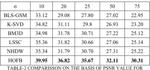
TABLE-2 COMPARISSON ON THE BASIS OF PSNR VALUE FOR THE IMAGE MONARCH CORRUPTED BY GAUSSIAN NOISE
MONARCH 512*512
σ 10 20 25 50 75
BLS-GSM 33.79 29.77 28.55 25.94 22.82
K-SVD 33.74 30.00 28.91 25.34 22.81 BM3D 34.12 30.35 29.25 25.82 23.91 LSSC 34.49 30.71 29.52 26.54 24.76 NHDW 34.48 30.72 29.49 26.72 24.99
HOFB 39.95 37.11 36.28 34.50 33.88
TABLE-3 COMPARISSON ON THE BASIS OF PSNR VALUE FOR THE IMAGE LENA CORRUPTED BY GAUSSIAN NOISE
LENA 512*512
σ 10 20 25 50 75
BLS-GSM 35.24 32.24 31.26 28.19 26.45 K-SVD 35.63 32.67 31.67 28.61 26.85 BM3D 35.93 33.05 32.07 29.05 27.25
LSSC 35.83 32.91 31.88 28.87 27.16
NHDW 35.89 32.99 32.02 29.06 27.39
HOFB 39.92 37.07 36.23 34.19 33.35
TABLE-4 COMPARISSON ON THE BASIS OF PSNR VALUE FOR THE IMAGE STRAW CORRUPTED BY GAUSSIAN NOISE
STRAW 512*512
σ 10 20 25 50 75
BLS-GSM 30.51 26.26 24.99 21.53 19.99 K-SVD 30.99 26.95 25.70 21.52 19.45
BM3D 30.92 27.08 25.89 22.41 20.72
LSSC 31.51 27.50 26.21 23.05 21.62
NHDW 31.70 27.72 26.68 23.38 21.91
Comparison of proposed method with the help of graph
10 15 20 25 30 35 40
0 10 20 30 40 50 60 70 80 90 100 noise PS N R
Leena with gaussian noise
Hierarchical Dictionary Learning Proposed
10 15 20 25 30 35 40
0 10 20 30 40 50 60 70 80 90 100 noise PS N R
barbara with gaussian noise
Hierarchical Dictionary Learning Proposed
10 15 20 25 30 35 40
0 10 20 30 40 50 60 70 80 90 100 noise PSN R
monarch with gaussian noise
Hierarchical Dictionary Learning Proposed
10 15 20 25 30 35 40
0 10 20 30 40 50 60 70 80 90 100 noise PSN R
straw with gaussian noise
Hierarchical Dictionary Learning Proposed
10 15 20 25 30 35 40
0 10 20 30 40 50 60 70 80 90 100 noise PS N R
straw with salt and pepper noise
Hierarchical Dictionary Learning Proposed
10 15 20 25 30 35 40
0 10 20 30 40 50 60 70 80 90 100 noise PSN R
Leena with salt and pepper noise
Hierarchical Dictionary Learning Proposed
10 15 20 25 30 35 40
0 10 20 30 40 50 60 70 80 90 100 noise PS N R
barbara with salt and pepper noise
Hierarchical Dictionary Learning Proposed
10 15 20 25 30 35 40
0 10 20 30 40 50 60 70 80 90 100 noise PS N R
monarch with salt and pepper noise
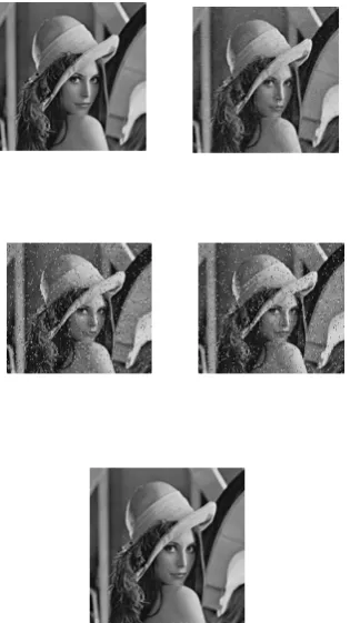
Fig. 3. De-noising results for the image “Barbara” with σ = 25 (Gaussian noise).
Fig. 4. De-noising results for the image “straw” with σ = 50 (Gaussian noise).
TABLE-5 COMPARISSON ON THE BASIS OF PSNR VALUE FOR THE IMAGE BARBARA CORRUPTED BY UNIFORM NOISE
BARBARA 512*512
α 10 20 30 40
BLS-GSM 34.10 27.99 24.34 23.29 K-SVD 35.13 29.89 26.64 24.47
BM3D 36.43 32.53 29.85 29.77 LSSC 36.72 32.53 29.85 29.77 NHDW 36.69 33.49 31.73 30.33
HOFB 41.00 37.97 37.35 35.84
TABLE-6 COMPARISSON ON THE BASIS OF PSNR VALUE FOR THE IMAGE LENA CORRUPTED BY UNIFORM NOISE
LENA 512*512
α 10 20 30 40
BLS-GSM 34.03 30.61 28.95 27.33
K-SVD 35.39 31.76 29.41 27.72 BM3D 36.84 34.10 32.52 31.44 LSSC 36.41 32.88 31.27 29.05 NHDW 36.53 34.99 32.88 31.75
HOFB 46.07 41.59 41.39 39.58
TABLE-7 COMPARISSON ON THE BASIS OF PSNR VALUE FOR THE IMAGE MONARCH CORRUPTED BY UNIFORM NOISE
MONARCH 512*512
α 10 20 30 40
BLS-GSM 33.15 29.32 25.34 24.69
K-SVD 34.50 29.62 27.21 25.63 BM3D 35.82 31.51 29.56 28.32 LSSC 35.81 30.99 29.68 27.98 NHDW 35.94 31.82 29.91 28.66
HOFB 42.94 39.90 37.87 36.17
TABLE-8 COMPARISSON ON THE BASIS OF PSNR VALUE FOR THE IMAGE STRAW CORRUPTED BY UNIFORM NOISE
STRAW 512*512
α 10 20 30 40
BLS-GSM 32.22 26.85 23.21 22.08 K-SVD 31.89 26.12 22.78 19.96
BM3D 33.46 28.07 25.71 24.30 LSSC 33.23 27.37 24.55 23.38 NHDW 33.51 28.44 26.23 24.75
Fig 4. De-noising results for the image “Lena” with α= 40 (Uniform noise).
Fig. 5. De-noising results for the image “Monarch” with a = 30 (uniform noise).
IV. CONCLUSION
A unique algorithm for Image De-noising has been proposed. It overcomes the major shortcomings of noisy image and de-noises the image to correct extent. Experimental results show that it works better than the other methods. We have got better PSNR values than the other methods discussed. The methodology of the given work uses Scaled Conjugate Gradient Algorithm for detecting and removing of noise from the given image.
ACKNOWLEDGEMENT
The author would like to thank the RIMT Institutes, Mandi Gobindgarh, Fatehgarh Sahib, Punjab, India. Author would also wish to thank editors and reviewers for their valuable suggestions and constructive comments that help in bringing out the useful information and improve the content of paper.
REFERENCES
1) J. Hui-Yan, C. Zhen-Yu, H. Yan, Z. Xiao-Jie Zhou; C. Tian-You. “Research on image denoising methods based on wavelet transform and rolling-ball algorithm”. Proceedings of the International Conference on Wavelet Analysis and Pattern Recognition, Beijing, China, 2007, pp. 1604-1607
2) Jing-Qing Zhao. Research on the algorithm of image de-noising based on wavelet transform [J]. Science and Technology innovation herald, 2009 NO.35.
3) M.Aharon and M.Elad. Image de-noising via sparse and redundant representations over learned dictionaries. IEEE Transactions on Image Processing, 15(12):3736–3745, December 2006
4) A. A. Bharath and J. Ng, “A steerable complex wavelet construction and its application to image de-noising,” IEEE Trans. Image Processing, Vol. 14, No. 7, pp. 948–959, 2005.
5) J. Zhong and R. Ning, “Image denoising based on wavelets and multifractals for singularity detection,” IEEE Trans. Image Processing, Vol. 14, No. 10, pp. 1435–1447, 2005.
6) H. Choi and R. G. Baraniuk, (2004) “Multiple wavelet basis image denoising using Besov ball projections,” IEEE Signal Processing Letters, Vol. 11, No. 9, 2004, pp. 717–720.
7) Z. Tongzhou; W. Yanli R. Ying; L. Yalan “Approach of Image Denoising Based on Discrete Multi-wavelet Transform International Workshop on Intelligent Systems and Applications, 2009, pp: 1-4. 8) L. Dalong , S. Simske, R.M. Mersereau. “Image Denoising Through
Support Vector Regression. Proceedings of IEEE International Conference on Image Processing, Vol. 4, 2007, pp. 425-428. 9) J. Hui-Yan, C. Zhen-Yu, H. Yan, Z. Xiao-Jie Zhou; C. Tian-You.
“Research on image denoising methods based on wavelet transform and rolling-ball algorithm”. Proceedings of the International Conference on Wavelet Analysis and Pattern Recognition, Beijing, China, 2007,pp. 1604-1607.
10) J. Xu, K. Zhang, M. Xu, and Z. Zhou. An adaptive threshold method for image denoising based on wavelet domain. Proceedings of SPIE, the International Society for Optical Engineering,7495:165, 2009. 11) J. Portilla, V. Strela, M.J. Wainwright, and E.P. Simoncelli. Image
denoising using scale mixtures of Gaussians in the wavelet domain. Image Processing, IEEE Transactions on, 12(11):1338–1351, 2003. 12) F. Luisier, T. Blu, and M. Unser. A new SURE approach to image
denoising: Interscale orthonormal wavelet thresholding. IEEE Transactions on Image Processing, 16(3):593–606, 2007.