Diffusion Matrices from Algebraic-Geometry Codes with Efficient SIMD
Implementation
?Daniel Augot1,2, Pierre-Alain Fouque3,4, and Pierre Karpman1,5,2 1 Inria, France
2 LIX — École Polytechnique, France 3 Université de Rennes 1, France 4 Institut universitaire de France, France 5 Nanyang Technological University, Singapore
{daniel.augot,pierre.karpman}@inria.fr,[email protected]
Abstract. This paper investigates large linear mappings with very good diffusion and efficient software implementations, that can be used as part of a block cipher design. The mappings are derived from linear codes over a small field (typicallyF24) with a high dimension (typically 16) and a high minimum distance. This results in diffusion matrices with equally high dimension and a large branch number. Because we aim for parameters for which no MDS code is known to exist, we propose to use more flexible algebraic-geometrycodes.
We present two simple yet efficient algorithms for the software implementation of matrix-vector multi-plication in this context, and derive conditions on the generator matrices of the codes to yield efficient encoders. We then specify an appropriate code and use its automorphisms as well as random sampling to find good such matrices.
We provide concrete examples of parameters and implementations, and the corresponding assembly code. We also give performance figures in an example of application which show the interest of our ap-proach.
Keywords: Diffusion matrix, algebraic-geometry codes, algebraic curves, SIMD, vector implementation, SHARK.
1 Introduction
The use ofMDSmatrices over finite fields as a linear mapping in block cipher design is an old trend, followed by many prominent algorithms such as theAES/Rijndaelfamily [6]. These matrices are called MDS as they are derived frommaximum distance separablelinear error-correcting codes, which achieve the highest minimum distance possible for a given length and dimension. This no-tion of minimum distance coincides with the one ofbranch numberof a mapping [6], which is a measure of the effectiveness of a diffusion layer. MDS matrices thus have an optimal diffusion, in a cryptographic sense, which makes them attractive for cipher designs.
The good security properties that can be derived from MDS matrices are often counter-balanced by the cost of their computation. The standard matrix-vector product is quadratic in the dimension of the vector, and finite field operations are not always efficient. For that reason, there is often a focus on finding matrices allowing efficient implementations. For instance, theAESmatrix is circu-lant and has small coefficients. More recently, thePHOTONhash function [8] introduced the use of matrices that can be obtained as the power of a companion matrix, which sparsity may be useful in lightweight hardware implementations. The topic of finding such so-called recursive diffusion lay-ers has been quite active in the past years, and led to a series of paplay-ers investigating some of their various aspects [17,22,2]. One of the most recent developments shows how to systematically con-struct some of these matrices from BCH codes [1]. This allows in particular to concon-struct very large recursive MDS matrices, for instance of dimension 16 overF28. This defines a linear mapping over a full 128-bit block with excellent diffusion properties, at a moderate hardware implementation cost. As interesting as it may be in hardware, the cost in software of a large linear mapping tends to make these designs rather less attractive than more balanced solutions. An early attempt to use a large matrix was the block cipherSHARK, aRijndaelpredecessor [15]. It is a 64-bit cipher which
uses an MDS matrix of dimension 8 overF28for its linear diffusion. The usual technique for imple-menting such a mapping in software is to rely on a table of precomputed multiples of the matrix rows. However, table-based implementations now tend to be frown upon as they may lead to tim-ing attacks[20], and this could leave ciphers with a structure similar toSHARK’s without reasonable software implementations when resistance to these attacks is required. Yet, such designs also have advantages of their own; their diffusion acts on the whole state at every round, and therefore makes structural attacks harder, while also ensuring that many S-Boxes are kept active. Additionally, the simplicity of the structure makes it arguably easier to analyze than in the case of most ciphers.
Our contributions. In this work, we revisit the use of aSHARKstructurefor block cipher design and endeavour to find good matrices and appropriate algorithms to achieve both a linear mapping with very good diffusion and efficient software implementations that are not prone to timing attacks. To be more specific on this latter point, we target software running on 32 or 64-bit CPUs featuring an SIMD vector unit.
An interesting way of trying to meet both of these goals is to decrease the size of the field from F28 toF24. However, according to the MDS conjecture, there is no MDS code over F24 of length greater than 17, and no such code is known [14]. Because a diffusion matrix of dimensionn is typically obtained from a code of length 2n, MDS matrices overF24 are therefore restricted to di-mensions less than 8. Hence, the prospect of finding an MDS matrix overF24 diffusing on more than 8×4=32 bits is hopeless. Obviously, 32 bits is not enough for a large mappingà laSHARK. We must therefore search for codes with a slightly smaller minimum distance in the hope that they can be made longer.
Our proposed solution to this problem is to usealgebraic-geometry codes[21], as they precisely offer this tradeoff. One way of defining these codes is as evaluation codes on algebraic curves; thus our proposal brings a nice connection between these objects and symmetric cryptography. Although elliptic and hyperelliptic curves are now commonplace in public-key cryptography, we show a rare application of an hyperelliptic curve to the design of block ciphers. We present a spe-cific code of length 32 and dimension 16 over F24 with minimum distance 15, which is only 2 less than what an MDS code would achieve. This lets us deriving a very good diffusion matrix on 16×4=64 bits in a straightforward way. Interestingly, this matrix can also be applied to vectors over an extension ofF24such asF28, while keeping the same good diffusion properties. This allows for instance to increase the diffusion to 16×8=128 bits.
We also study two simple yet efficient algorithms for implementing the matrix-vector multi-plication needed in aSHARK structure, when avector permuteinstruction is available. From one of these, we derive conditions on the matrix to make the product faster to compute, in the form of a cost function; we then search for matrices with a low cost, both randomly, and by using au-tomorphisms of the code and of the hyperelliptic curve on which it is based. The use of codes automorphisms to derive efficient encoders is not new [10,5], but it is not generally applied to the architecture and dimensions that we consider in our case.
We conclude this paper by presenting examples of performance figures of assembly implemen-tations of our algorithms when used as the linear mapping of a block cipher.
2 Preliminaries
We noteF2m the finite field with 2m elements. We often considerF24, and implicitly use this spe-cific field if not mentioned otherwise. W.l.o.g. we use the representationF24 ∼=F2[α]/(α4+α+1). We freely use “integer representation” for elements ofF24 by writingn ∈{0 . . . 15}=P3i
=0ai2i to represent the elementx∈F24=P3
i=0aiα
i.
Bold variables denote vectors (in the sense of elements of a vector space), and subscripts are used to denote theirithcoordinate, starting from zero. For instance,x=(1, 2, 7) andx2=7. IfMis a matrix ofncolumns, we callmi=(Mi,j, j=0 . . .n−1) the row vector formed from the coefficients of itsithrow. We use angle brackets “〈” and “〉” to write ordered sets.
Arrays, or tables, (in the sense of software data structures) are denoted by regular variables such asxorT, and their elements are accessed by using square brackets. For instance,T[i] is the ithelement of the tableT, starting from zero.
We conclude with two definitions.
Definition 1 (Systematic form and dual of a code) LetCbe an[n,k,d]F2mcode of length n,
dimen-sion k and minimum distance d with symbols inF2m. A generator matrix forC is insystematic form
if it is of the form(Ik A), with Ik the identity matrix of dimension k and A a matrix of k rows and n−k columns. A systematic generator matrix for thedualofC is given by(In−k At).
Definition 2 (Branch number [6]) Let A be the matrix of a linear mapping overF2m, andwm(x)be
the number of non-zero positions of the vectorxoverF2m. Then thedifferential branch numberof A is
equal tominx6=0(wm(x)+wm(A(x))), and thelinear branch numberof A is equal tominx6=0(wm(x)+ wm(At(x))).
Note that ifAis such that (Ik A) is a generator matrix of a code of minimum distancedwhich dual code has minimum distanced0, then A has a differential (resp. linear) branch number ofd (resp.d0).
3 Efficient algorithms for matrix-vector multiplication
This section presents software algorithms for matrix-vector multiplication overF24. We focus on square matrices of dimension 16. This naturally defines linear operations on 64 bits, which can also be extended to 128 bits, as it will be made clear in §5. Both cases are a common block size for block ciphers.
Targeted architecture. The algorithms in this section target CPUs featuring vector instructions, in-cluding in particular avector shuffleinstruction such as Intel’spshufbfrom the SSSE3 instruction set extension [11]. These instructions are now widespread and have already been used success-fully in fast cryptographic implementations, seee.g.[9,19,3]. We mostly considered SSSE3 when designing the algorithms, but other processor architectures do feature vector instructions. This is for instance the case of ARM’s NEON extensions, which may also yield efficient implementations, seee.g.[4]. We do not consider these explicitly in this paper, however.
Because it plays an important role in our algorithms, we briefly recall the semantics ofpshufb. Thepshufbinstruction takes two 128-bit inputs1. The first (the destination operand) is anxmmSSE vector register which logically represents a vector of 16 bytes. The second (the source operand) is either a similarxmmregister, or a 128-bit memory location. The result of callingpshufbx y is to overwrite the inputxwith the vectorx0defined by:
x0[i]=
½
x[by[i]c4] if the most significant bit ofy[i] is not set
0 otherwise
whereb·c4denotes truncation to the 4 least significant bits. This instruction allows to arbitrarily
shufflea vector according to a mask, with possible repetition and omission of some of the vector values2. Notice that this instruction can also be used to perform 16 parallel 4-to-8-bit table lookups: let us callT this table; take as first operand topshufbthe vectorx=(T[i],i=0 . . . 15), as second operand the vectory=(a,b,c,d, . . .) on which to perform the lookup; then we see that the first byte of the result isx[y[0]]=T[a], the second isx[y[1]]=T[b], etc.
Finally, there is a three-operand variant of this instruction in the more recent AVX instruction set and onward [11], which allows not to overwrite the first operand.
Targeted properties. In this paper we focus solely on algorithms that can easily be implemented in a way that makes them immune to timing-attacks [20]. Specifically, we consider the matrix as a known constant but the vector as a secret, and we wish to perform the multiplication without secret-dependent branches or memory accesses. It might not always be important to be immune (or even partially resistant) to this type of attacks, but we consider that it should be important for any cryptographic primitive or structure to possibly be implemented in such a way. Hence we try to find efficient such implementations for theSHARKstructure and therefore for dense matrix-vector multiplications.
We now go on to describe the algorithms. In all of the remainder of this section,xandyare two (column) vectors ofF1624, andM a matrix ofM16(F24). We first briefly recall the principle of table implementations, which are unsatisfactory when timing attacks are taken into account.
3.1 Table implementation
We wish to computey=M·x. The idea behind this algorithm is to use table lookups to perform the equivalent multiplicationyt=xt·Mt,i.e.yt=P15
i=0xi·(m
t)i (where (mt)iis theithrow ofMt). This can be computed efficiently by tabulating beforehand the productsλ·(mt)i,λ∈F24(resulting in 16 tables, each of 16 entries of 64 bits), and then for each multiplication by accessing the table for (mt)i at the indexxiand summing all the retrieved table entries together. This only requires 16 table lookups per multiplication. However, the memory accesses depend on the value ofx, which makes this algorithm inherently vulnerable to timing attacks.
Note that there is a more memory-efficient alternative implementation of this algorithm which consists in computing each termλ·(mt)iwith a singlepshufbinstruction instead of using a table-lookup. In that case, only the 16 multiplication tables need to be stored, but their accesses still depend on the secret valuex.
3.2 A generic constant-time algorithm
We now describe our first algorithm, which can be seen as a variant of table multiplication that is immune to timing attacks. The idea consists again in computing the right multiplicationyt =
xt·Mt,i.e.yt=P15 i=0xi·(m
t)i. However, instead of tabulating the results of the scalar multiplication of the matrix rows (mt)i, those are always recomputed, in a way that does not explicitly depend on the value of the scalar.
Description of algorithm 1. We give the full description of Alg. 1 in appendix A.1, and focus here on the intuition. We want to perform the scalar multiplicationλ·zfor an unknown scalarλand a known, constant vectorz, overF24. Let us write λas the polynomialλ3·α3+λ2·α2+λ1·α+
λ0with coefficients inF2. Then, the result ofλ·zis simplyλ3·(α3·z)+λ2·(α2·z)+λ1·(α·z)+
λ0·z. Thus we just need to precompute the productsαi·z, select the right ones with respect to
the binary representation ofλ, and add these together. This can easily be achieved thanks to a broadcastfunction defined as:
broadcast(x,i)n= ½
1n if theithbit ofxis set 0n otherwise
where1nand0ndenote then-bit binary string made all of one and all of zero respectively. The full algorithm then just consists in using this scalar-vector multiplication 16 times, one for each row of the matrix.
Implementation of algorithm 1 with SSSE3 instructions. We now consider how to efficiently im-plement algorithm 1 in practice. The only non-trivial operation is thebroadcastfunction, and we show that this can be performed with only one or twopshufbinstructions.
To computebroadcast(λ,i)64, withλa 4-bit value, we can use a singlepshufbwith first operand
x, such thatx[j]=111111112 if theithbit of j is set and 0 otherwise, and with second operand
y=(λ,λ,λ, . . .). The result ofpshufbx yis indeed (x[λ],x[λ], . . .) which is164if theithbit ofλis set, and064otherwise, that isbroadcast(λ,i)64.
In practice, the vectorxcan conveniently be constructed offline and stored in memory, but the vectorymight not be readily available before performing this computation3. However, it can easily be computed thanks to an additionalpshufb. Alternatively, if the above computation is done with a vectory=(λ, ?, ?, . . .) instead (with ? denoting unknown values) and callz its result (x[λ], ?, ?, . . .), then we havebroadcast(λ,i)n=pshufbz(0, 0, . . .).
In the specific case of matrices of dimension 16 overF24, one can take advantage of the 128-bit widexmmregisters by interleaving, say, 8·xwith 4·x, and 2·xwithx, and by computing a slightly more complex version of thebroadcastfunction broadcast(x,i,j)2n which interleavesbroadcast(x,i)n withbroadcast(x,j)n. In that case, an implementation of one step of algorithm 1 only requires two broadcastcalls, two logicaland, folding back the interleaved vectors (which only needs a couple of logical shift and exclusive or), and adding the folded vectors together. We give a snippet of such an implementation in appendix B.1.
3.3 A faster algorithm exploiting matrix structure
The above algorithm is already reasonably efficient, and has the advantage of being completely generic w.r.t. the matrix. Yet, better solutions may exist in more specific cases. We present here an alternative that can be much faster when the matrix possesses a particular structure.
The idea behind this second algorithm is to take advantage of the fact that in a matrix-vector product, the same constant values may be used many times in finite-field multiplications. Hence, we try to take advantage of this fact by performing those in parallel. The fact that we now focus on multiplications by constants (i.e.matrix coefficients) allows us to compute these multiplications with a singlepshufbinstead of using the process from algorithm 1.
Description of algorithm 2. We give the full description of Alg. 2 in appendix A.2, and focus here on the intuition. Let us first consider a small example, and computeM·xdefined as:
1 0 2 2 3 1 2 3 2 3 3 2 0 2 3 1 · x0 x1 x2 x3 . (1)
It is obvious that this is equal to: x0 x1 0 x3
+2·
x2 x2 x0 x1
+ 2·
x3 0 x3 0
+3·
0 x0 x1 x2
+3·
0 x3 x2 0 ,
where both the constant multiplications of the vector (x0 x1 x2 x3)t and the shuffles of its coef-ficients can be computed with a singlepshufbinstruction each, while none of these operations directly depends on the value of the vector. This type of decomposition can be done for any matrix, but the number of operations depends on the value of its coefficients.
We now sketch one way of obtaining an optimal decomposition as above. We consider a ma-trix product M·xwithM constant andxunknown, wherexis seen as the formal arrangement of variablesxi. Let us defineS(M,γ) as one of the minimal sets of shuffles of coefficients ofx, such that there exists a unique vectorz∈S(M,γ) withzi =xj iffMi,j =γ. For instance, in the above example, we haveS(M, 2)={(x2 x2x0x1)t, (x30x30)t}. Equivalently, we could have taken
S(M, 2)={(x3x2x30)t, (x20x0x1)t}. These sets are straightforward to compute from this particu-lar matrix, and so are they in the general case.
From the definition ofS, it is clear that we haveM·x=P γ∈F∗
24
P
s∈S(M,γ)γ·s. Once the values of the setsS have been determined, it is clear that we only need to compute this sum to get our result, and this is precisely what this second algorithm does.
Cost of algorithm 2. The cost of computing a matrix-vector product with algorithm 2 depends on the coefficients of the matrix, since the size of the setsS(M,γ) depends both on the density of the matrix and of how its coefficients are arranged.
If we assume that a vector implementation of this algorithm is used, and if the dimension and the field of the matrix are well chosen, we can assume that both the scalar multiplication ofxby a constant and its shuffles can be computed with a singlepshufband a few ancillary instructions. Hence, we can define a cost function for a matrix with respect to its implementation with algo-rithm 2 to becost2(M)=¡ Pγ∈F24∗1(S(M,γ))+#S(M,γ)
¢
−1(S(M, 1)), where1(E) withE a set is one ifE 6= ;, and zero otherwise. We may notice that #S(M,γ) is equal to the maximum number of occurrence ofγin a single row ofM, and thecost2function is therefore easy to compute. As an example the cost of the matrixMfrom equation 1 is 7.
In order to find matrices that minimize thecost2function, we would like to minimize the sum of the maximum number of occurrence ofγfor everyγ∈F∗24. A simple observation is that for matrices with the same number of non-zero coefficients, this amount is minimal when every row can be deduced by permutation of a single one; an important particular case being the one ofcirculant matrices. More generally, we can heuristically hope that the cost of a matrix will be low if all of its rows can be deduced by permutation of a small subset thereof.
We can try to estimate the minimum cost for an arbitrary dense circulant matrix of dimension 16 overF24. It is fair to assume that nearly all of the values ofF24 should appear as coefficients of such a matrix, 14 of them needing a multiplication. Additionally, 15–16 permutations are needed if all the rows are to be different. Hence we can assume that thecost2function of such a matrix is about 30.
Finally, let us notice that special cases of this algorithm have already been used for circulant matrices, namely in the case of theAES MixColumnmatrix [9,3].
Implementation of algorithm 2 with SSSE3 instructions. The implementation of algorithm 2 is quite straightforward. We give nonetheless a small code snippet in appendix B.2.
3.4 Performance
4 Diffusion matrices from algebraic-geometry codes
In this section, we present so-called algebraic-geometry codes and show how they can give rise to diffusion matrices with interesting parameters. We also focus on implementation aspects, and investigate how to find matrices with efficient implementations with respect to the algorithms of §3, and in particular algorithm 2.
4.1 A short introduction to algebraic-geometry codes
We first briefly present the concept of algebraic-geometry codes (or AG codes for short), which are linear codes, and how to compute their generator matrices. Because the codes are linear, these encoders are matrices. We do not give a complete description of AG codes, and refer toe.g.[21] for a more thorough treatment. We present a class of AG codes as a generalization of Reed-Solomon (RS) codes. We give a quick presentation of RS codes in appendix C for the reader not familiar with them.
We see AG codes asevaluation codes: to build the codeword for a messagew, we considerwas a function, and the codeword as a vector of values of this function evaluated on some “elements”. In our case, the elements are points of the two-dimensional affine spaceA2(F2m), and the functions
are polynomials in two variables, that is elements ofF2m[x,y]. The core idea of AG codes is to
con-sider points of a (smooth) projective curve of the projective spaceP2(F2m) and functions from the
curve’s function space. Points at infinity are never included in the (ordered) set of points. However, points of the curve at infinityareuseful in defining the curve’s function (sub)-space, which is why we do consider the curve in the projective space instead of the affine one.
We first give the definition of the Riemann-Roch space in the special case where it is defined from a divisor made of a single point at infinity. We refer toe.g.[18] or [21] for a more complete and rigorous definition.
Definition 3 (Riemann-Roch space) LetX be a smooth projective curve ofP2(F2m)defined by the
homogeneous polynomial p(x,y,z), and let p0(x,y)be the dehomogenized of p. We defineF
2m[X]=
F2m[x,y]/p0as thecoordinate ringofX, and its corresponding quotient fieldF2m(X)as thefunction
fieldofX. Assume Q is the only point ofX at infinity, and let r be a positive integer. The Riemann-Roch spaceL(r Q)is the set of all functions ofF2m(X)with poles only at Q of order less than r . This
is a finite-dimensionalF2m-vector-space. Furthermore, letoQ(x)andoQ(y)be the order of the poles
of x and y in Q4, then a basis ofL(r Q)is formed by all the monomial functions xiyj that are such that i·oQ(x)+j·oQ(y)≤r .
This space is particularly important because of the following theorem, which links its dimen-sion with the genus ofX [18].
Theorem 1 (Riemann and Roch) LetL(r Q)be a Riemann-Roch space defined onX, and g be the genus ofX. We havedim(L(r Q))≥r+1−g , with equality when r>2g−2.
We have also mentioned earlier that a basis for a spaceL(r Q) can be computed as soon as the order of the poles ofxand y inQ are known, and the dimension of the space can obviously be computed from the basis. In practice, computing oQ(x) and oQ(y) can be done from a local parameterization ofxandy inQ. Both this parameterization and the values oQ(x) and oQ(y) can easily be obtained from a computational algebra software such as Magma. Again, we refer to [21] for more details.
We are now ready to define a simple class of AG codes.
Definition 4 (Algebraic-Geometry codes) Let X be a smooth projective curve of P2(F2m) with a
unique point Q at infinity, and call#X its number of affine points (that is not counting Q). As-sume that#X ≥n and let r be s.t.dim(L(r Q))=k, and call(f0, . . . ,fk−1)one basis of this space. We
define the codeword of the[n,k,d]F2m algebraic-geometry codeCAGassociated with the messagem
as the vectorP
i=0...k−1(mi·fi(pj),j=0 . . .n−1), where P= 〈p0, . . . ,pn−1〉is an ordered set of points
ofX/{Q}. The codeCAGis the set of all such codewords.
These codes have the following properties: for fixed parametersnandk and a curveX, there are¡#X
n ¢
·n!equivalent codes, which corresponds to the number of possible ordered setsP; it is also obvious that the maximal length of a code overX is #X. We also have the following proposi-tion [21]:
Proposition 1 LetCAG be a code of length n and dimension k, and let r be an integer such that dim(L(r Q))=k. Then the minimum distance ofCAGis at least n−r . IfXis of genus g and r>2g−2, this is equal to n−((k−1)+g)=n−k−g+1. Therefore, the “gap” between this code and an MDS code of the same length is g . The same holds for the dual code.
The minimum distance of AG codes thus depends on the genus of the curves used to define them. Because the maximal number of points on a curve increases with its genus, there is a tradeoff be-tween the length of a code and its minimum distance.
Construction of a generator matrix of an AG code. Once the parameters of a code have been fixed, including the ordered setP, one just has to specify a basis ofL(r Q), and to form the encoding matrixM∈Mk,n(F2m) obtained by evaluating this basis onP. A useful basis is one such that the
encoding matrix is in systematic form, but it does not necessarily exist for anyP. Note however that in the case of MDS codes (such as RS codes) this basis always exists whatever the parameters and the choice ofP: this is because in this case every minor ofMis of full rank [14]. When such a basis exists, it is easy to find as one just has to start from an arbitrary basis and to compute the reduced row echelon form of the matrix thus obtained.
Example 1: An AG code from an elliptic curve. We give parameters for a code built from the curve defined onP2(F24) by the homogeneous polynomialx2z+xz2=y3+y z2, or equivalently defined on
A2(F24) byx2+x=y3+y. It is of genus 1, and hence it is an elliptic curve. It has 25 points, including one point at infinity, the pointQ=[1 : 0 : 0]; the order of the poles ofxandyinQare respectively 3 and 2. From this, a basis for the spaceL(12Q) can easily be obtained. This space has dimension 12+1−g=12, and can be used to define a [24, 12, 12]F24 code by evaluation over the affine points
of the curve. This allows to define a matrix of dimension 12 overF24, which diffuses over 12×4=48 bits and has a differential and linear branch number of 12.
Example 2: An AG code from an hyperelliptic curve. We increase the length of the code by using a curve with a larger genus. We give parameters for a rather well-known code, built from the curve defined onP2(F24) by the homogeneous polynomialx5=y2z+y z4. This curve has 33 points, in-cluding one point at infinity, the pointQ =[0 : 1 : 0]; the order of the poles ofx and y inQ are respectively 2 and 5. From this, a basis for the spaceL(17Q) can easily be defined. This space has dimension 17+1−g=16, and can be used to define a [32, 16, 15]F24 code by evaluation over the
affine points of the curve. This code has convenient parameters for defining diffusion matrices: from a generator matrix in systematic form (I16 A), we can extract the matrixA, which naturally diffuses over 64 bits and has a differential and linear branch number of 15. Furthermore, the code isself-dual, which means thatA is orthogonal: A·At =I16. The inverse of A is therefore easy to compute.
The problem for the rest of the section is now to find good point ordersPfor the hyperelliptic code of Ex. 2 such that efficient encoders can be constructed thanks to algorithm 2 of §3.3. For convenience, we nameCH E any of the codes equivalent to the one of Ex. 2.
4.2 Compact encoders using code automorphisms
We consider matrices in systematic form (I16 A). For dense matrices, Alg. 2 tends to be most effi-cient when all the rows of a matrix can be deduced by permutation of one of them, or more gener-ally of a small subset of them. Our objective is thus to find matrices of this form.
The main tool we use to achieve this goal areautomorphismsofCH E. Let us first give a defini-tion. (In the following,Sndenotes the group of permutations ofnelements.)
Definition 5 (Automorphisms of a code) The automorphism group Aut(C)of a codeC of length n is a subgroup ofSnsuch thatπ∈Aut(C)⇒(c∈C ⇒π(c)∈C).
Because we consider here the codeCH E which is an evaluation code, we can equivalently de-fine its automorphisms as being permutations of the points on which the evaluation is performed. Ifπis an automorphism ofCH E, if {O0, . . . ,Ol} are its orbits, and if the code is defined with a point orderPsuch that for each orbit all of its points are neighbours in the orderP, then the effect ofπ on a codeword ofCH E is to cyclically permute its coordinates along each orbit.
To see that this is useful, assume that there is an automorphismπwith two orbitsO0andO1of sizen/2 each. Then, ifM=(In/2 A) is obtained with point orderP = 〈O0,O1〉, each row ofMcan be obtained by the repeated action ofπon, say,m0, and it follows thatAis circulant (and therefore has a low cost w.r.t. algorithm 2). More generally, if an automorphism can be found such that it has orbits of size summing up ton/2, the corresponding matrixMcan be deduced from a small set of rows. We give two toy examples with Reed-Solomon codes, which can easily be verified.
π: F24 →F24, x7→8x. This automorphism hasO0= 〈1, 8, 12, 10, 15〉andO1= 〈2, 3, 11, 7, 13〉for orbits, among others. The systematic matrix for the [10, 5, 6]F24 code obtained with the points in
that order is then such that A is circulant and obtained from the cyclic permutation of the row (12, 10, 2, 6, 3).
π: F24 →F24, x7→7x. This automorphism hasO0= 〈1, 7, 6〉,O1= 〈2, 14, 12〉,O2= 〈4, 15, 11〉, and
O3= 〈8, 13, 5〉for orbits, among others. The systematic matrix for the [12, 6, 7]F24code obtained with
the points in that order is then of the form µ
I303 A B 03 I3C D
¶
withA,B,CandDcirculant matrices. It can thus be obtained by cyclic permutation of only two rows.
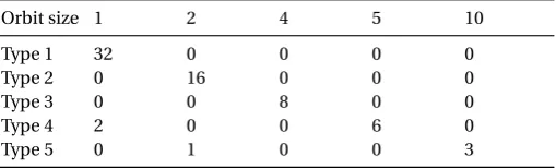
Application toCH E. Automorphisms ofCH E are quite harder to find than ones of RS codes. They can however be found within automorphisms of the curveX on which it is based [18]. This is quite intuitive, as these will precisely permute points on the curve, which are the points on which the code is defined. We mostly need to be careful to ensure that the point at infinity is fixed by these automorphisms. We considered the degree-one automorphisms ofX described by Duursma [7]. They have two generators:π0: F224→F224, (x,y)7→(ζx,y) withζ5=1, andπ1(a,b): F
2
24→F224, (x,y)7→ (x+a,y+a8x2+a4x+b4), with (a,b) an affine point ofX. These generators span a group of order 160. When considering their orbit decomposition, the break-up of the size of the orbits can only be of one of five types, given in Table 1.
From these automorphisms, it is possible to define a partitions ofPin two sets of size 16, which are union of orbits. We may therefore hope to obtain systematic matrices of the type we are looking for. Unfortunately, after an extensive search5, it appears that orderingP in this fashionneverresults in obtaining a systematic matrix. We recall that indeed, because AG codes are not MDS, it is not always the case that computing the reduced row echelon form of an arbitrary encoding matrix yields a systematic matrix.
5Both onC
Table 1.Possible combination of orbit sizes of automorphisms ofCH E spanned byπ0andπ1. A numbernin col.c means that an automorphism of this type hasnorbits of sizec.
Orbit size 1 2 4 5 10
Type 1 32 0 0 0 0
Type 2 0 16 0 0 0
Type 3 0 0 8 0 0
Type 4 2 0 0 6 0
Type 5 0 1 0 0 3
Extending the automorphisms with the Frobenius mapping. We extend the previous automor-phisms with the Frobenius mappingθ: F224 →F224, (x,y)7→(x2,y2); this adds another 160 auto-morphisms forX. However, these will not anymore be automorphisms for thecodeCH E in gen-eral, and we will therefore obtain matrices of a form slightly different from what we first hoped to achieve.
The global strategy is still the same, however, and consists in ordering the points along orbits of the curve automorphisms. By using the Frobenius, new combinations of orbits are possible, no-tably 4 of size 8. We study below the result of orderingPalong the orbits of one such automorphism. We take the example ofσ=θ◦σ2◦σ1, withσ1: (x,y)7→(x+1,y+x2+x+7),σ2: (x,y)7→(12x,y), andθthe Frobenius mapping. The key observation is that in this case, onlyσ0andσ4are automor-phisms ofCH E. Note that not all orbits orderings ofσforP yield a systematic matrix. However, unlike as above, we were able to find some orders that do. In these cases, the right matrix “A” of the full generator matrix (I16A) is of the form:
(a0,a1,a2,a3,σ4(a0),σ4(a1),σ4(a2),σ4(a3),a8,a9,a10,a11,σ4(a8),σ4(a9),σ4(a10),σ4(a11))t,
witha0, . . . ,a3,a8, . . . ,a11 row vectors of dimension 16. For instance, the first and fifth row of one such matrix are:
a0=(5, 2, 1, 3,8, 5, 1, 5, 12, 10, 14, 6,7, 11, 4, 11) a4=σ4(a0)=(8, 5, 1, 5, 5, 2, 1, 3,7, 11, 4, 11, 12, 10, 14, 6).
We give the full matrix in appendix D.1. We have therefore partially reached our goal of being able to describeAfrom a permutation of a subset of its rows. However this subseta0, . . . ,a3,a8, . . . ,a11 is not small, as it is of size 8 —half of the matrix dimension. Consequently, these matrices have a moderate cost according to thecost2function, when implemented with algorithm 2, but it is not minimal. Interestingly, all the matrices of this form that we found have the same cost of 52.
4.3 Fast random encoders
We conclude this section by presenting the results of a very simple random search for efficient encoders ofCH E with respect to algorithm 2. Unlike the above study, this one does not exploit any kind of algebraic structure. Indeed, the search only consists in repeatedly generating a random permutation of the affine points of the curve, building a matrix for the code with the corresponding point order, tentatively putting it in systematic form (I16A), and if successful evaluating thecost2 function from §3.3 onA. We then collect matrices with a minimum cost.
5 Applications and performance
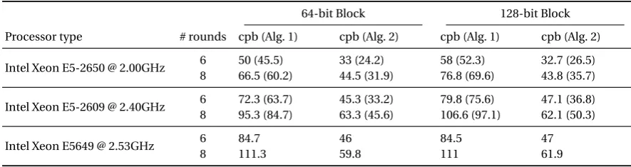
This last section presents the performance of straightforward assembly implementations of both of our algorithms when applied to a fast encoder of the codeCH E from §4. More precisely, we consider the diffusion matrix “MH16” of appendix D.2; it is of dimension 16 over F24 and has a differential and linear branch number of 15. We do this study in the context of block ciphers, by assuming thatMH16is used as the linear mapping of two ciphers with aSHARKstructure: one with 4-bit S-Boxes and a 64-bit block, and one with 8-bit S-Boxes and a 128-bit block. What we wish to measure in both cases is the speed in cycles per byte of such hypothetical ciphers, so as to be able to gauge the efficiency of this linear mapping and of the resulting ciphers. In order to do this, we need to estimate how many rounds would be needed for the ciphers to be secure.
Basic statistical properties of a 64-bit block cipher with 4-bit S-Boxes andMH16as a linear
map-ping. We use standardwide-trailconsiderations to study differential and linear properties of this cipher [6]. This is very easy to do thanks to the simple structure of the cipher. The branch number ofMH16is 15, which means that at least 15 S-boxes are active in any two rounds of a differential path or linear characteristic. The best 4-bit S-boxes have a maximum differential probability and a maximal linear bias of 2−2(seee.g.[16,13]). By using such S-boxes, one can upper-bound the prob-ability of a single differential path or linear characteristic for 2nrounds by 2−2·15n. This is smaller than 2−64as soon asn>2. Hence we conjecture that 6 to 8 rounds are enough to make a cipher resistant to standard statistical attacks.
If one were to propose a concrete cipher, a more detailed analysis would of course be needed, especially w.r.t. more dedicated structural attacks. However, it seems reasonable to consider at a first glance that 8 rounds would indeed be enough to bring adequate security. It is only 2 rounds less thanAES-128, which uses a round with comparatively weaker diffusion. Also, 6 rounds might be enough. Consequently, we present software performance figures for 6 and 8 rounds of such an hypothetical 64-bit cipher with 4-bit S-Boxes in Table 2, on the left. We include data both for a strict SSSE3 implementation and for one using AVX extensions, which can be seen to bring a considerable benefit. Note that the last round is complete and includes the linear mapping, unlike e.g.AES. Also, note that the parallel application of the S-Boxes can be implemented very efficiently with a singlepshufb, and thus has virtually no impact on the speed.
Basic statistical properties of a 128-bit block cipher with 8-bit S-Boxes andMH16 as a linear
mapping. Although the codeCH E from which the matrixMH16is built was initially defined with
F24as an alphabet, this latter can be replaced by an algebraic extension ofF24 such asF28, to yield a codeCH E0with the same parameters, namely a [32, 16, 15]F28 code. Indeed, by using a suitable
representation such asF24∼=F2[α]/(α4+α3+α2+α+1);F28∼=F24[t]/(t2+t+α)6, an element ofF28 is represented as a degree-one polynomialat+boverF24. It follows that the minimum weight of a codewordw=(ait+bi),i ∈{0 . . . 31} ofCH E0is at least equal to the minimum weight of words (ai),i=0 . . . 31 and (bi),i∈{0 . . . 31}. If those are taken among codewords ofCH E, their minimum weight is 15, and thus so is the one ofw. It is also possible to efficiently compute the multiplication byMH16overF28from two computations overF24: because the coefficients ofMH16are inF24, we haveMH16·(ait+bi)=(MH16·(ai)·t)+(MH16·(bi)). As a result, applyingMH16toF28 has only twice the cost of applying it toF24, while effectively doubling the size of the block.
From wide-trail considerations, the resistance of such a cipher to statistical attacks is compar-atively even better than when using 4-bit S-Boxes, when an appropriate 8-bit S-Box is used. For instance, theAESS-box has a maximal differential probability and linear bias of 2−6[6]. This im-plies that the probability of a single differential path or linear characteristic for 2nrounds is upper-bounded by 2−6·15n, which is already much smaller than 2−128as soon asn>1. Again, 8 rounds of such a cipher should bring adequate security, and 6 rounds might be enough. We provide perfor-mance figures for both an SSSE3 and an AVX implementation in Table 2, on the right. However, in
the case of 8-bit S-Boxes, the S-Box application is rather more complex and expensive a step than with 4-bit S-Boxes. In these test programs, we decided to use the efficient vector implementation of theAESS-Box from Hamburg [9].
Table 2.Performance of software implementations of the hypothetical 64 and 128-bit cipher, in cycles per byte (cpb). Figures in parentheses are for an AVX implementation (when applicable).
64-bit Block 128-bit Block
Processor type # rounds cpb (Alg. 1) cpb (Alg. 2) cpb (Alg. 1) cpb (Alg. 2)
Intel Xeon E5-2650 @ 2.00GHz 6 50 (45.5) 33 (24.2) 58 (52.3) 32.7 (26.5) 8 66.5 (60.2) 44.5 (31.9) 76.8 (69.6) 43.8 (35.7)
Intel Xeon E5-2609 @ 2.40GHz 6 72.3 (63.7) 45.3 (33.2) 79.8 (75.6) 47.1 (36.8) 8 95.3 (84.7) 63.3 (45.6) 106.6 (97.1) 62.1 (50.3)
Intel Xeon E5649 @ 2.53GHz 6 84.7 46 84.5 47
8 111.3 59.8 111 61.9
Discussion. The performance figures given in Table 2 are average for a block cipher. For instance, it compares favourably with the optimized vector implementations of 64-bit ciphersLEDandPiccolo in sequential mode from [3], which run at speeds between 70 and 90 cpb., depending on the CPU. It is however slower than Hamburg’s vector implementation ofAES, with reported speeds of 6 to 22 cpb. (9 to 25 for the inverse cipher) [9,19].
6 Conclusion
We revisited theSHARKstructure by replacing the MDS matrix of its linear diffusion layer by a ma-trix built from an algebraic-geometry code. Although this code is not MDS, it has a very high min-imum distance, while being defined overF24 instead ofF28. This allows to reduce the size of the coefficients of the matrix from 8 to 4 bits, and has important consequences for efficient implemen-tations of this linear mapping. We studied algorithms suitable for a vector implementation of the multiplication by this matrix, and how to find matrices that are most efficiently implemented with those algorithms. Finally, we gave performance figures for assembly implementations of hypothet-icalSHARK-like ciphers using this matrix as a linear layer.
This work provided the first generalizations ofSHARKthat are not vulnerable to timing attacks as is the original cipher, and also the first generalization to 128-bit blocks. It also showed that even if not the fastest, such potential design could be implemented efficiently in software.
As a future work, it would be interesting to investigate how to use the full automorphism group of the code to design matrices with a lower cost. In that case, we would not restrict ourselves to derive the rows from a single row and the powers of asingleautomorphism, but could use several independent automorphisms instead.
Acknowledgments
References
1. Augot, D., Finiasz, M.: Direct Construction of Recursive MDS Diffusion Layers using Shortened BCH Codes. In: FSE. Lecture Notes in Computer Science (to appear), Springer. Available athttps://www.rocq.inria.fr/secret/ Matthieu.Finiasz/research/2014/augot-finiasz-fse14.pdf.
2. Augot, D., Finiasz, M.: Exhaustive Search for Small Dimension Recursive MDS Diffusion Layers for Block Ciphers and Hash Functions. In: ISIT, IEEE (2013) 1551–1555
3. Benadjila, R., Guo, J., Lomné, V., Peyrin, T.: Implementing lightweight block ciphers on x86 architectures. In Lange, T., Lauter, K., Lisonek, P., eds.: Selected Areas in Cryptography. Volume 8282 of Lecture Notes in Computer Science., Springer (2013) 324–351
4. Bernstein, D.J., Schwabe, P.: NEON Crypto. In Prouff, E., Schaumont, P., eds.: CHES. Volume 7428 of Lecture Notes in Computer Science., Springer (2012) 320–339
5. Chen, J.P., Lu, C.C.: A Serial-In-Serial-Out Hardware Architecture for Systematic Encoding of Hermitian Codes via Gröbner Bases. IEEE Transactions on Communications52(8) (2004) 1322–1332
6. Daemen, J., Rijmen, V.: The Design of Rijndael: AES — The Advanced Encryption Standard. Information Security and Cryptography. Springer (2002)
7. Duursma, I.: Weight distributions of geometric Goppa codes. Transactions of the American Mathematical Society
351(9) (1999) 3609–3639
8. Guo, J., Peyrin, T., Poschmann, A.: The PHOTON Family of Lightweight Hash Functions. In Rogaway, P., ed.: CRYPTO. Volume 6841 of Lecture Notes in Computer Science., Springer (2011) 222–239
9. Hamburg, M.: Accelerating AES with Vector Permute Instructions. In Clavier, C., Gaj, K., eds.: CHES. Volume 5747 of Lecture Notes in Computer Science., Springer (2009) 18–32
10. Heegard, C., Little, J., Saints, K.: Systematic Encoding via Gröbner Bases for a Class of Algebraic-Geometric Goppa Codes. IEEE Transactions on Information Theory41(6) (1995) 1752–1761
11. Intel Corporation: Intel® 64 and IA-32 Architectures Software Developer’s Manual. (March 2012)
12. Knudsen, L.R., Wu, H., eds.: Selected Areas in Cryptography, 19th International Conference, SAC 2012, Windsor, ON, Canada, August 15-16, 2012, Revised Selected Papers. In Knudsen, L.R., Wu, H., eds.: Selected Areas in Cryptography. Volume 7707 of Lecture Notes in Computer Science., Springer (2013)
13. Leander, G., Poschmann, A.: On the Classification of 4 Bit S-Boxes. In Carlet, C., Sunar, B., eds.: WAIFI. Volume 4547 of Lecture Notes in Computer Science., Springer (2007) 159–176
14. MacWilliams, F.J., Sloane, N.J.A.: The Theory of Error-Correcting Codes. North-Holland Mathematical Library. North-Holland (1978)
15. Rijmen, V., Daemen, J., Preneel, B., Bosselaers, A., Win, E.D.: The Cipher SHARK. In Gollmann, D., ed.: FSE. Volume 1039 of Lecture Notes in Computer Science., Springer (1996) 99–111
16. Saarinen, M.J.O.: Cryptographic Analysis of All 4×4-Bit S-Boxes. In Miri, A., Vaudenay, S., eds.: Selected Areas in Cryptography. Volume 7118 of Lecture Notes in Computer Science., Springer (2011) 118–133
17. Sajadieh, M., Dakhilalian, M., Mala, H., Sepehrdad, P.: Recursive Diffusion Layers for Block Ciphers and Hash Func-tions. In Canteaut, A., ed.: FSE. Volume 7549 of Lecture Notes in Computer Science., Springer (2012) 385–401 18. Stichtenoth, H.: Algebraic Function Fields and Codes. 2 edn. Volume 254 of Graduate Texts in Mathematics. Springer
(2009)
19. Suzaki, T., Minematsu, K., Morioka, S., Kobayashi, E.: TWINE: A Lightweight Block Cipher for Multiple Platforms. [12] 339–354
20. Tromer, E., Osvik, D.A., Shamir, A.: Efficient Cache Attacks on AES, and Countermeasures. J. Cryptology23(1) (2010) 37–71
21. Van Lint, J.H.: Introduction to Coding Theory. 3 edn. Volume 86 of Graduate Texts in Mathematics. Springer (1999) 22. Wu, S., Wang, M., Wu, W.: Recursive Diffusion Layers for (Lightweight) Block Ciphers and Hash Functions. [12]
355–371
A Algorithms for matrix-vector multiplication
A.1 Broadcast-based algorithm
Algorithm 1Broadcast-based matrix-vector multiplication Input: x∈F16
24,M∈M16(F24)
Output: y=xt·Mt Offline phase 1: fori∈{0 . . . 15}do
2: 8mi←α3·mi
3: 4mi←α2·mi
4: 2mi←α·mi
5: end for
Online phase 6: y←064
7: fori∈{0 . . . 15}do
8: γ8
i←8mi∧64broadcast(xi, 3)64
9: γ4i←4mi∧64broadcast(xi, 2)64 10: γ2
i←2mi∧64broadcast(xi, 1)64 11: γ1i←mi∧64broadcast(xi, 0)64 12: γi←γ8i+γ4i+γ2i+γ1i
13: y←y+γi
14: end for
15: return y
A.2 Shuffle-based algorithm
The shuffle-based algorithm for matrix-vector multiplication of §3.3 is given in Algorithm 2.
Algorithm 2Shuffle-based matrix-vector multiplication Input: x∈F16
24,M∈M16(F24)
Output: y=M·x
Offline phase 1: fori∈{1 . . . 15}do
2: si[ ]←S(M,i).Initialize the array siwith one of the possible sets of shufflesS(M,i)
3: end for
Online phase 4: y←064
5: fori∈{1 . . . 15}do
6: forj<#sido
7: y←y+i·si[j]
8: end for
9: end for
10: return y
B Excerpts of assembly implementations of matrix-vector multiplication
B.1 Excerpt of an implementation of algorithm 1
; c l e a n i n g m a s k
cle : dq 0 x 0 f 0 f 0 f 0 f 0 f 0 f 0 f 0 f , 0 x 0 f 0 f 0 f 0 f 0 f 0 f 0 f 0 f
; m a s k for the s e l e c t i o n of v , 2 v
oe1 : dq 0 x f f 0 f f 0 0 0 f f 0 f f 0 0 0 , 0 x f f 0 f f 0 0 0 f f 0 f f 0 0 0
; m a s k for the s e l e c t i o n of 4 v , 8 v
oe2 : dq 0 x f 0 f 0 f 0 f 0 0 0 0 0 0 0 0 0 , 0 x f f f f f f f f 0 f 0 f 0 f 0 f
; m0 and 2 m0 i n t e r l e a v e d
c01 : dq 0 x 9 1 a 7 e f a 7 6 c 1 2 6 c b 5 , 0 x 9 1 2 4 f d 9 1 c b 3 6 3 6 d 9
; 4 m0 and 8 m0 i n t e r l e a v e d
c02 : dq 0 x 2 4 e f d 9 e f b 5 4 8 b 5 a 7 , 0 x 2 4 8 3 9 1 2 4 5 a c b c b 1 2
; e t c .
c12 : dq 0 x 8 3 2 4 6 c 8 3 3 6 0 0 5 a b 5 , 0 x b 5 9 1 4 8 3 6 7 e 2 4 a 7 7 e c21 : dq 0 x f d d 9 b 5 1 2 2 4 2 4 b 5 9 1 , 0 x a 7 3 6 1 2 e f 1 2 2 4 3 6 d 9 c22 : dq 0 x 9 1 1 2 a 7 4 8 8 3 8 3 a 7 2 4 , 0 x e f c b 4 8 d 9 4 8 8 3 c b 1 2
; [ ... ]
; m a c r o for one m a t r i x row m u l t i p l i c a t i o n and a c c u m u l a t i o n ; ( n a s m s y n t a x )
; 1 is i n p u t
; 2 , 3 , 4 , 5 are s t o r a g e ; 6 is c o n s t a n t z e r o ; 7 is a c c u m u l a t o r ; 8 is i n d e x
% m a c r o m _ 1 _ r o w 8
; s e l e c t s the r i g h t double - m a s k s
m o v d q a %2 , [ oe1 ] m o v d q a %3 , [ oe2 ] p s h u f b %2 , %1 p s h u f b %3 , %1
; s h i f t the i n p u t for the n e xt r o u n d
p s r l d q %1 , 1
; e x p a n d
p s h u f b %2 , %6 p s h u f b %3 , %6
; s e l e c t the r ow s w i t h the double - m a s k s
p a n d %2 , [ c01 + % 8 * 1 6 * 2 ] p a n d %3 , [ c02 + % 8 * 1 6 * 2 ]
; s h i f t and xor the r o w s t o g e t h e r
m o v d q a %4 , %2 m o v d q a %5 , %3 p s r l q %2 , 4 p s r l q %3 , 4 p x o r %4 , %5 p x o r %2 , %3
; a c c u m u l a t e e v e r y t h i n g
p x o r %2 , %4 p x o r %7 , %2 % e n d m a c r o
; the i n p u t is in xmm0 , w i t h o n l y the f o u r lsb of e a c h by t e set
_ m 6 4 :
; c o n s t a n t z e r o
p x o r xmm5 , x m m 5
; a c c u m u l a t o r
p x o r xmm6 , x m m 6 . m a i n s t u f f :
m _ 1 _ r o w xmm0 , xmm1 , xmm2 , xmm3 , xmm4 , xmm5 , xmm6 , 0 m _ 1 _ r o w xmm0 , xmm1 , xmm2 , xmm3 , xmm4 , xmm5 , xmm6 , 1 m _ 1 _ r o w xmm0 , xmm1 , xmm2 , xmm3 , xmm4 , xmm5 , xmm6 , 2
; [ ... ]
. f i n :
; the r e s u l t is in xmm0 , and s t i l l of the s a m e f o r m
p a n d xmm6 , [ cle ] m o v d q a xmm0 , x m m 6 ret
B.2 Excerpt of an implementation of algorithm 2
; m u l t i p l i c a t i o n t a b l e s ( in the o r d e r w h e r e we n e e d t h e m )
t t i m 2 : dq 0 x 0 e 0 c 0 a 0 8 0 6 0 4 0 2 0 0 , 0 x 0 d 0 f 0 9 0 b 0 5 0 7 0 1 0 3 t t i m 8 : dq 0 x 0 d 0 5 0 e 0 6 0 b 0 3 0 8 0 0 , 0 x 0 1 0 9 0 2 0 a 0 7 0 f 0 4 0 c
; s h u f f l e s
; 0 xff for not s e l e c t e d n i b b l e s ( it w i l l z e r o t h e m )
p p 1 0 : dq 0 x 0 0 0 5 0 0 0 5 0 7 0 4 0 d 0 2 , 0 x 0 f 0 1 0 4 0 a 0 3 0 6 0 8 0 9 p p 1 1 : dq 0 x f f f f 0 e 0 c 0 e 0 b f f f f , 0 x f f 0 b 0 8 f f 0 4 0 c f f f f p p 1 2 : dq 0 x f f f f f f 0 e f f 0 d f f f f , 0 x f f f f f f f f f f f f f f f f
p p 2 0 : dq 0 x 0 5 0 3 0 6 0 7 0 6 0 2 0 4 0 e , 0 x 0 4 0 8 0 1 0 c 0 1 0 0 0 b 0 4 p p 2 1 : dq 0 x 0 c 0 e 0 9 0 9 f f 0 3 0 7 f f , 0 x 0 b f f 0 2 0 e f f f f 0 d f f p p 2 2 : dq 0 x f f f f f f 0 f f f 0 a f f f f , 0 x f f f f f f f f f f f f f f f f
p p 3 0 : dq 0 x f f f f f f 0 2 f f 0 9 f f 0 9 , 0 x 0 a f f f f 0 4 f f f f f f 0 2 p p 3 1 : dq 0 x f f f f f f 0 4 f f 0 e f f 0 a , 0 x 0 e f f f f 0 f f f f f f f 0 f
; [ ... ]
; 2 u s e f u l m a c r o s ( n a s m s y n t a x )
; 1 is the l o c a t i o n of the vector ,
; 2 is s t o r a g e for the m u l t i p l i e d thingy , ; 3 is the c o n s t a n t i n d e x
% m a c r o v e c _ m u l 3
m o v d q a %2 , [ t t i m 2 + % 3 * 1 6 ] p s h u f b %2 , %1
m o v d q a %1 , %2 % e n d m a c r o
; 1 is the a c c u m u l a t o r ,
; 2 is the m u l t i p l i e d vector ,
; 3 is s t o r a g e for the s h u f f l e d thingy , ; 4 is the i n d e x for the s h u f f l e
% m a c r o p p _ a c c u 4 m o v d q a %3 , %2
p s h u f b %3 , [ p p 1 0 + % 4 * 1 6 ] p x o r %1 , %3
% e n d m a c r o
; the i n p u t is in xmm0 , w i t h o n l y the f o u r lsb of e a c h by t e set
_ m 6 4 :
p x o r xmm1 , x m m 1 ; i n i t the a c c u m u l a t o r
. m a i n s t u f f :
; 1 .x
p p _ a c c u xmm1 , xmm0 , xmm2 , 0 p p _ a c c u xmm1 , xmm0 , xmm2 , 1 p p _ a c c u xmm1 , xmm0 , xmm2 , 2
; 2 .x
v e c _ m u l xmm0 , xmm2 , 0
p p _ a c c u xmm1 , xmm0 , xmm2 , 3 p p _ a c c u xmm1 , xmm0 , xmm2 , 4 p p _ a c c u xmm1 , xmm0 , xmm2 , 5
; 3 .x
v e c _ m u l xmm0 , xmm2 , 1
p p _ a c c u xmm1 , xmm0 , xmm2 , 6 p p _ a c c u xmm1 , xmm0 , xmm2 , 7
; [ ... ]
. f i n :
; the r e s u l t is in xmm0 , and s t i l l of the s a m e f o r m
m o v d q a xmm0 , x m m 1 ret
C A short introduction to Reed-Solomon codes
Definition 6 (Reed-Solomon codes) LetCRS be an[n,k,d]F2m Reed-Solomon code of length n,
messagemof dimension k is defined as the vector(m(pi),i=0 . . .n−1), wheremis seen as the poly-nomialP
i=0...k−1mi·xi ofF2m[x]of degree at most k−1, and where P= 〈p0, . . . ,pn−1〉is an ordered
set of n elements ofF2m, n≤2m. The code is the set of all such codewords.
These codes have the following properties: for fixed parametersnandk, there are¡2m
n ¢
·n!equivalent codes, which corresponds to the number of possible ordered setsP; the minimal distancedof a code of parametersnandkis at leastn−(k−1)=n−k+1. This is because a polynomial of degree k−1 has at most k−1 zeros, and hence any codeword except the all-zero word is non-zero on at leastn−(k−1) positions. Because this bound reaches the Singleton bound, RS codes are MDS codes; finally, it is obvious that the maximal length of an RS code overF2mis 2m.
D Examples of diffusion matrices of dimension 16 over F24
D.1 A matrix of cost 52
The following matrix for the diffusion part ofCH E was found thanks to the automorphisms from §4.2, based on the Frobenius mapping. It has cost 52, and both a differential and a linear branch
number of 15.
5 2 1 3 8 5 1 5 12 10 14 6 7 11 4 11 2 2 4 1 5 12 2 1 9 15 8 11 7 6 9 3 1 4 4 3 1 2 15 4 5 13 10 12 9 6 7 13 3 1 3 3 5 1 4 10 14 2 14 8 15 13 7 6 8 5 1 5 5 2 1 3 7 11 4 11 12 10 14 6 5 12 2 1 2 2 4 1 7 6 9 3 9 15 8 11 1 2 15 4 1 4 4 3 9 6 7 13 5 13 10 12 5 1 4 10 3 1 3 3 15 13 7 6 14 2 14 8 12 9 5 14 7 7 9 15 7 6 11 3 15 5 13 7 10 15 13 2 11 6 6 13 6 6 7 9 5 10 2 14 14 8 10 14 4 9 7 7 11 7 7 6 13 2 8 4
6 11 12 8 11 3 13 6 3 9 6 6 7 14 4 12 7 7 9 15 12 9 5 14 15 5 13 7 7 6 11 3 11 6 6 13 10 15 13 2 5 10 2 14 6 6 7 9 4 9 7 7 14 8 10 14 13 2 8 4 11 7 7 6 11 3 13 6 6 11 12 8 7 14 4 12 3 9 6 6
D.2 A matrix of cost 43
The following matrix, for the same code, was found by randomly testing permutations of the points of the curve. It has cost 43, and so does its transpose.
11 6 1 6 10 14 10 9 13 3 3 12 9 15 2 9 6 12 0 4 2 8 9 2 5 11 9 5 4 1 15 6 9 11 2 2 1 11 13 15 13 3 2 1 14 1 3 10 0 0 9 8 11 6 2 1 11 10 15 10 10 15 1 14 13 13 3 15 3 1 11 2 9 2 10 14 1 11 1 2
1 9 8 4 14 10 2 5 15 2 12 12 9 10 1 9 5 9 11 2 15 1 12 4 6 0 6 4 5 8 2 9 1 4 14 9 13 2 10 12 0 6 6 9 2 0 11 10 13 10 3 9 2 15 6 6 11 1 9 9 12 14 10 3
0 10 6 12 11 0 4 9 1 14 10 2 9 2 13 6 2 0 5 6 9 0 1 5 15 12 13 15 1 11 13 11 11 2 10 1 1 15 0 8 0 9 14 10 10 6 11 15 12 14 10 11 3 10 6 0 5 11 1 8 2 9 2 3 15 2 2 5 1 10 9 4 1 8 9 9 12 10 14 12 15 1 12 5 13 11 0 6 2 5 11 1 15 0 9 13 5 6 11 0 2 9 14 11 12 10 3 2 8 10 3 1
It can easily be obtained as follows. First, define a basis ofL(17Q), for instance: (1,x,x2,y,x3,x y, x4,x2y,x5,x3y,x6,x4y,x7,x5y,x8,x6y). Then, arrange the affine points of the curve on whichCH E is defined in the order7:〈(8, 7), (13, 2), (4, 5), (0, 0), (14, 5), (15, 6), (7, 3), (1, 7), (2, 2), (11, 3), (3, 3), (10, 7), (6, 4), (5, 5), (9, 5), (12, 6), (3, 2), (11, 2), (12, 7), (13, 3), (4, 4), (0, 1), (1, 6), (7, 2), (9, 4), (6, 5), (2, 3), (5, 4), (15, 7), (10, 6), (14, 4), (8, 6)〉. Finally, evaluate the basis ofL(17Q) on these points (this defines a matrix of 16 rows and 32 columns), and compute the reduced row echelon form of this matrix; the right square matrix of dimension 16 of the result is the matrix above.
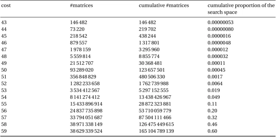
E Statistical distribution of the cost of matrices ofCH E
Table 3.Statistical distribution of the cost of 238randomly-generated generator matrices ofCH E.
cost #matrices cumulative #matrices cumulative proportion of the search space
43 146 482 146 482 0.00000053
44 73 220 219 702 0.00000080
45 218 542 438 244 0.0000016
46 879 557 1 317 801 0.0000048
47 1 978 159 3 295 960 0.000012
48 5 559 814 8 855 774 0.000032
49 21 512 707 30 368 481 0.00011
50 93 289 020 123 657 501 0.00045
51 356 848 829 480 506 330 0.0017
52 1 282 233 658 1 762 739 988 0.0064
53 3 534 412 567 5 297 152 555 0.019
54 8 141 274 412 13 438 426 967 0.049
55 15 433 896 914 28 872 323 881 0.11
56 24 837 735 898 53 710 059 779 0.20
57 33 794 051 687 87 504 111 466 0.32
58 38 971 338 149 126 475 449 615 0.46
59 38 629 339 524 165 104 789 139 0.60