Secure Computation on Floating Point Numbers
Mehrdad Aliasgari, Marina Blanton, Yihua Zhang, and Aaron Steele Department of Computer Science and Engineering
University of Notre Dame
{maliasga,mblanton,yzhang16,asteele2}@nd.edu
Abstract
Secure computation undeniably received a lot of attention in the recent years, with the shift toward cloud computing offering a new incentive for secure computation and outsourcing. Surprisingly little attention, however, has been paid to computation with non-integer data types. To narrow this gap, in this work we develop efficient solutions for computation with real numbers in floating point representation, as well as more complex operations such as square root, logarithm, and exponentiation. Our techniques are information-theoretically secure, do not use expensive cryptographic techniques, and can be applied to a variety of settings. Our experimental results also show that the techniques exhibit rather fast performance and in some cases outperform operations on integers.
1
Introduction
As today’s society is becoming increasingly connected with a growing amount of information avail-able in the digital form, the amount of personal, sensitive, or otherwise private information collected and stored is constantly growing. When dealing with such information, one of the most technically challenging issues arises when private or sensitive information needs to be used in computation without revealing unnecessary information. This applies to both personal and proprietary data.
The desire to carry out computation in a privacy-preserving manner without revealing any in-formation about the private inputs throughout the computation has been a topic of research since the first general secure function evaluation result was introduced by Yao in his seminal work [43]. Despite a large amount of attention from the research community, secure computation techniques are not commonly used in practice because of their complexity and overhead. The recent progress in the performance of secure multi-party computation techniques, however, shows that secure compu-tation can be very fast (e.g., millions of operations performed on the order of seconds by Sharemind on a LAN [7]).
While it is well known that any computable function can be evaluated securely (e.g., as a Boolean or arithmetic circuit), recently a substantial amount of literature (see, e.g., [19, 20, 32] among many others) has been dedicated to optimizing secure realizations of commonly used op-erations. This is not surprising considering that, for instance, a substantial performance gain in secure implementation of a comparison operation (be it based on garbled circuits, homomorphic encryption, or secret sharing techniques) leads to a significant performance improvement of a very large number of functions which might be used in secure computation. To date, however, the great majority of techniques treat computation on the integers, while there are undeniably limitations to integer arithmetic. This work makes a step toward expanding the available techniques to other data types, and in particular develops techniques for secure multi-party computation on real numbers in the floating point representation. While prior literature [23, 17, 24] offers a limited number of techniques for real number computation, we are not aware of any work that develops a suite of techniques for floating point computation or secure multi-party techniques for complex functions such as logarithm, square root, and exponentiation. Such techniques are therefore the focus of this work.
Because performance of secure computation techniques is crucial, our techniques are designed to optimize both the overall and round complexity of the solutions. In addition, in order to provide a fair assessment of the performance of operations on different numeric data types in the multi-party framework, we implement a number of operations for integer, fixed point, and floating point real values and evaluate their performance. To the best of our knowledge, these are the first experimental results not only for floating point representation, but also for fixed point operations, which we carry out in a standard threshold linear secret sharing setting. To summarize, our contributions are as follows:
• Design of efficient secure multi-party techniques for floating point computation in a standard linear secret sharing framework.
• Design of efficient (and fast converging) protocols for complex operations over real numbers (square root, logarithm, and exponentiation).
• Evaluation of the developed and existing techniques for integer, fixed point, and floating point arithmetic.
Security of our protocols is shown in both passive (also known as semi-honest or honest-but-curious) and active (malicious) adversarial models.
2
Preliminaries
2.1 Framework
Throughout this work we assume that parties P1, . . ., Pn are connected by pair-wise secure authenticated channels. Each input and output party also establishes secure channels with P1
throughPn. With a (n, t)-secret sharing scheme, any private value is secret-shared amongnparties such that anyt+1 shares can be used to reconstruct it, whiletor fewer shares reveal no information about the shared value, i.e., it is perfectly protected in the information-theoretic sense. Therefore, the values of n and t should be chosen such that an adversary is unable to corrupt more than t
computational parties.
In a secret sharing scheme that we utilize, any linear combination of secret-shared values can be performed by each computational party locally, without any interaction, but multiplication of two secret-shared values requires communication between all of them. In other words, if we let [x] denote that value x is secret-shared among P1, . . ., Pn, operations [x] + [y], [x] +c, and c[x] are performed by each Pi locally on its shares of x and y, while computation of [x][y] is interactive. We also use notationOutput([a]) to denote that all parties broadcast their shares ofawhich allows them to reconstruct the value of a. All operations are assumed to be performed in a fieldFq for a small primeq greater than the maximum value that needs to be used in the computation (defined later).
Performance of secure computation techniques is of grand significance, as protecting secrecy of data throughout the computation often incurs substantial computational costs. For that reason, besides security, efficient performance of the developed techniques is one of our prime goals. Nor-mally, performance of a protocol in the current setting is measured in terms of two parameters: (i) the number of interactive operations (multiplications, distributing shares of a private value or open-ing a secret-shared value) necessary to perform the computation, and (ii) the number of sequential interactions, or rounds. We employ the same metrics throughout this work.
2.2 Related work
Prior work on general techniques for secure two- and multi-party computation is extensive, and its review is beyond the scope of this work. Prior work more closely related to ours primarily concentrates on techniques for integer computation and includes work on bit decomposition [19, 36, 42, 39], where a secret-shared value is converted to shares of the bits in its binary representation; comparison [19, 36, 26, 38], where the operands may or may not have to be given in the bit-decomposed form; addition and subtraction of bit bit-decomposed values [19, 8, 15]; and division [9, 13, 16, 30, 17, 12]. The majority of the above techniques concentrate on constant-round protocols (i.e., independent of the bit length of their operands), and the researchers over time gained notable performance improvement for some of the operations.
needed.
Recent implementations of secure multi-party techniques include [6, 5] and two-party techniques include [31, 33].
2.3 Building blocks
Our solutions rely on the following existing building blocks:
• [r] ← RandInt(k) allows the parties to generate shares of a random k-bit value [r] without any interaction (see, e.g., [17]) using what can be viewed as a distributed pseudo-random function.1
• [r]←RandBit() allows the parties to produce shares of a random bit [r] using one interactive operation.
• [c] ← XOR([a],[b]) computes exclusive OR of bits a and b as [a] + [b]−2[a][b] using one multiplication.
• [c]←OR([a],[b]) computes OR of bits aand bas [a] + [b]−[a][b].
• [b]←Inv([a]) computesb=a−1 (inFq). For a non-zeroathis operation can be implemented
using a single interaction, where the parties create a random [r], compute and openc=r·a
and set [b] =c−1[r].
• ([y1], . . .,[yn]) ← PreMul([x1], . . .,[xn]) computes prefix-multiplication, where on input a
se-quence of integers x1, . . ., xn, the output consists ofy1, . . ., yn, where eachyi =Qij=1xj. The most efficient implementation of this operation in our framework that we are aware of is due to Catrina and de Hoogh [15] that uses 2 rounds and 3n−1 interactive operations, but works only on non-zero elements of a field. Most of the cost is input independent and can be performed ahead of time (after precomputation the cost becomes ninteractive operations in 1 round).
• ([y1], . . .,[yn])←PreOR([x1], . . .,[xn]) computes prefix-OR of ninput bitsx1, . . ., xnand out-putsy1, . . .,ynsuch that eachyi=
Wi
j=1xj. One possible implementation from [15] uses 5n−1 interactive operations in 3 rounds, which after input-independent precomputation becomes 2n−1 interactive operations in 2 rounds.
• [b] ← EQ([x],[y], `) is an equality protocol that on input two secret-shared `-bit values x
and y outputs a bitb which is set to 1 iffx =y. Secure multi-party implementation of this operation in [15] uses another protocol [b]←EQZ([x0], `), which outputs bitb= 1 iff x0 = 0, by callingEQZ([x]−[y], `). EQ and EQZ use `+ 4 log` interactive operations2 in 4 rounds; after precomputation this becomes log(`) + 2 interactive operations in 3 rounds.
• [b]←LT([x],[y], `) is a comparison protocol that on input two secret-shared`-bit valuesxand
y outputs a bitb which is set to 1 iff x < y. Efficient implementations of this function also exist, e.g., we can use the comparison protocol from [15] with 4 rounds and 4`−2 interactive operations (or `+ 1 interactive operations in 3 rounds after precomputation). It similarly utilizes protocol [b]←LTZ([x0], `) which outputs 1 iff x0 <0 by callingLTZ([x]−[y], `).
1
More precisely, to produce a random integer without interaction, the parties generate it as the sum of random integers from [0,2k), producing a value longer thankbits long, the length of which depends on the number of parties
nand the threshold valuet.
2
• [y]← Trunc([x], `, m) computes b[x]/2mc, where ` is the length ofx. This operation can be efficiently implemented, e.g., using the techniques of [15], which require 4 rounds and 4m+ 1 interactive operations for this functionality, orm+ 2 interactive operations in 3 rounds after input-independent precomputation.
• [xm−1], . . .,[x0] ← BitDec([x], `, m) performs bit decomposition of m least significant bits of
x, where ` is the size of x. An efficient implementation of this functionality can be found in [17] that uses log(m) rounds andmlog(m) interactive operations (note that the complexity is independent of the size of its argument x).
• [a] ← FPDiv([x],[y], γ, f) performs division of floating point values x and y and produces floating point value x/y. It can be found in [17]. Hereγ is the total length of floating point representation and 2−f is the precision (i.e., there are γ−f and f bits before and after the radix point, respectively). The complexity of this function for γ = 2f is 3 log(γ) + 2θ+ 12 rounds and 1.5γlog(γ) + 2γθ+ 10.5γ+ 4θ+ 6 interactive operations, whereθ is the number of iterations equal to dlog(γ/3.5)e.
2.4 Security model
For each presented protocol, we define its secure functionality such that the parties carrying out the computation do not provide any input and do not receive any output. Instead, it is assumed that prior to the beginning of the computation the parties with inputs will secret-share their values among the parties carrying out the computation. Likewise, if the result of a computation is to be revealed to one or more parties, the computational parties will send their shares to the output parties who reconstruct the result. This allows for arbitrary composition of the protocols and their suitability for use in outsourced environments.
We next formally define security using the standard definition in secure multi-party computa-tion for semi-honest adversaries, i.e., those that follow the computacomputa-tion as prescribed, but might attempt to learn additional information about the data from the intermediate results. We prove our techniques secure in the semi-honest model and then show that standard techniques for making the computation robust to malicious behavior apply to our protocols as well.
Definition 1 Let partiesP1, . . ., Pnengage in a protocolπ that computes functionf(in1, . . ., inn) =
(out1, . . .,outn), where ini and outi denote the input and output of party Pi, respectively. Let VIEWπ(Pi) denote the view of participant Pi during the execution of protocol π. More precisely,
Pi’s view is formed by its input and internal random coin tossesri, as well as messagesm1, . . ., mk passed between the parties during protocol execution:
VIEWπ(Pi) = (ini, ri, m1, . . ., mk).
Let I ={Pi1, Pi2, . . ., Pit} denote a subset of the participants for t < n and VIEWπ(I) denote the
combined view of participants in I during the execution of protocol π (i.e., the union of the views of the participants inI). We say that protocolπ ist-private in presence of semi-honest adversaries if for each coalition of size at most t there exists a probabilistic polynomial time simulator SI such that
{SI(inI, f(in1, . . .,inn)} ≡ {VIEWπ(I),outI},
where inI=SPi∈I{ini}, outI =
S
3
New Building Blocks
Before proceeding with describing our solution for secure floating point arithmetic, we present new building blocks which are used in several of our protocols and can also be of independent interest. Such building blocks are:
• [b] ← Trunc([a], `,[m]) that performs truncation of its first argument [a] by an unknown number of bitsm, where`is the bitlength ofa. This operation is the same as division by an unknown power of 2. Note that a straightforward approach to implementing this functionality is to run Trunc([a], `, m) on all possible values of m < ` and then obliviously choose one of them. This approach, however, results in O(`2) interactive operations, while we are able to achieve notable O(`) in O(log log`) rounds. This, in particular, substantially outperforms general-purpose division. Our protocol is of independent interest and is used in this work in several types of operations on floating point numbers.
• [a0], . . .,[a`−1]←B2U([a], `) is a conversion procedure from a binary to unary representation.
It converts the first argumenta < `from a binary to unary bitwise representation, where the output is ` bits, a least significant bits of which are set to 1 and all others are set to 0. In this work,B2Uconstitutes a significant component of our truncation protocol by an unknown number of bits, and its efficiency helps us to achieve the claimed performance ofTrunc.
• [2a]← Pow2([a], `) raises 2 in the (unknown) power asupplied as the first argument, where the second argument ` specifies the length of the values. In particular, the bitlength of 2a cannot exceed `, which means thatashould be in the range [0, `). Pow2 is called from many protocols includingB2U, and is described next.
We implement [2a] ← Pow([a], `) as follows: The logic behind it is rather simple and consists of
first computing m=dlog`e least significant bits [am−1], . . .,[a0] of [a] (since the result of raising 2
in the power of a longer than log(`)-bit value cannot be represented) and computing the result as
Qm−1
i=0 (22
i
[ai] + 1−[ai]). This gives us complexity sub-linear in`.
[2a]←Pow2([a], `)
1. m← dlog`e;
2. [am−1], . . .,[a0]←BitDec([a], m, m);
3. ([x0], . . .,[xm−1])←PreMul(22
0
[a0] + 1−[a0], . . ., 22
m−1
[am−1] + 1−[am1]); 4. return [xm−1];
In addition to using this Pow2 protocol as a building block of Trunc and B2U, we utilize it to implement other functionalities in this work and it is thus of independent interest.
In the next protocol, binary-to-unary conversionB2U([a], `) below, we first callPow2([a], `). We then create a random (`+κ)-bit value r, the ` least significant bits of which are secret shared by the parties, and broadcastc= [2a] + [r] (steps 2 and 3). Hereκis a statistical security parameter, which is also used in many building blocks listed in section 2.3. The function Bits(c, `) in step 4 returns `least significant bits of (public) c. Given the bitsci’s of 2a blinded with a random value
r, in step 5 we compute XOR of ci and the corresponding bit ri of r and store the resulting bits as xi’s. As a result of this operation, we obtain that because a least significant bits of 2a are 0,
the bitsxi. As the next step in the computation, we execute PreORon the computed bits xi’s, as a result of which we obtain thataleast significant bitsy0, . . ., ya−1 are 0, while the remaining`−a
bits ya, . . ., y`−1 are all set to 1. This allows us to easily obtain bits of the unary representation of
aby returning the complement of each computed bit.
[a0], . . .,[a`−1]←B2U([a], `)
1. [2a]←Pow2([a], `);
2. fori= 0 to `−1 in parallel [ri]←RandBit(); 3. c←Output([2a] + 2`·RandInt(κ) +P`−1
i=02i[ri]);
4. (c`−1, . . ., c0)←Bits(c, `);
5. fori= 0 to `−1 in parallel [xi]←ci+ [ri]−2ci[ri]; 6. ([y0], . . .,[y`−1])←PreOR([x0], . . .,[x`−1]);
7. fori= 0 to `−1 in parallel [ai]←1−[yi]; 8. return [a0], . . .,[a`−1];
Lastly, we describe truncation Trunc([a], `,[m]) and provide its protocol below. In the solution, we first produce bit-wise unary representation of its argument [m] using B2U. Because B2U also computes [2m] at an intermediate step, we store that value as well instead of recomputing it. The computation starting from line 3 uses the structure of the regular truncation by a number of bits given in the clear as the starting point. In detail, we first choose ` random bits, form an m-bit randomr0and an (κ+`−m)-bit randomr00(without knowledge ofmin the clear), and broadcast the value ofaprotected with an (κ+`)-bit randomr= 2mr00+r0 (lines 3–6). After performing modulo reduction of the result (using all possible powers of 2 as the moduli), we obtainc00= (a+r) mod 2m (line 8). Becauseamod 2m=c00−r0+2md, wheredis a bit which equals to 1 ifamod 2m+r0 >2m, we need to compute the value ofdand compensate for the error. This is done on lines 9–10, where the returned result is (a−(amod 2m))2−m. Note that the output ofTruncis meaningful only when 0≤m < `.
[b]←Trunc([a], `,[m])
1. h[x0], . . .,[x`−1]i,[2m]←B2U([m], `);
2. [2−m]←Inv([2m]);
3. fori= 0 to `−1 in parallel [ri]←RandBit(); 4. [r0]←P`−1
i=02i[xi][ri];
5. [r00]←2`·RandInt(κ) +P`−1
i=02i(1−[xi])[ri];
6. c←Output([a] + [r00] + [r0]);
7. fori= 1 to `−1 in parallelc0i =cmod 2i; 8. [c00]←P`−1
i=1c0i([xi−1]−[xi]);
9. [d]←LT([c00],[r0], `);
10. [b]←([a]−[c00] + [r0])[2−m]−[d]; 11. return [b];
Note that because the protocol already computes amod 2m, we can use its steps to easily realize
Mod2m([a], `,[m]) function for computing modulo reduction for 2m, where m is secret shared. To accomplish this, all that is needed is to replace line 10 inTruncwith [b]←[c00]−[r0] + [2m][d].
4
Basic Operations in Floating Point Representation
4.1 Floating point representation
Today the floating point format is the most common representation for real numbers on computers due to its obvious precision advantages over fixed point or integer representation. Floating point representation consists of a fixed-precision significandvand an exponentpwhich specifies how the value is to be scaled (using a specified base), e.g., the value of the form v·2p when base is 2. To maximize precision and the number of representable values, floating point numbers are typically stored in normalized form, where the significand stores the leading non-zero bit and a fixed number of bits that follows. Then because 0 does not have such a representation, to preserve correctness of the computation, we choose to explicitly store with each value a bit which indicates whether the value is 0. For performance reasons we also store the sign bit separately; this prevents us from explicitly testing for 0 values and the sign during basic operations. We therefore represent each real valueu as a 4-tuple (v, p, z, s) with base 2, wherev is an `-bit significand, p is ak-bit exponent, z
is a bit which is set to 1 iff u = 0, andsis a sign bit which is set when the value is negative. We obtain thatu= (1−2s)(1−z)v·2p. When u= 0, we also maintain thatz= 1,v = 0, andp= 0. Each non-zero value is normalized, which in our representation means that the most significant bit of v is always set to 1 and therefore v ∈ [2`−1,2`). This is done by adjusting the (signed) exponentpaccordingly, which is from the range (−2k−1,2k−1) that we denote byZhki. The mapping from negative values to elements of the field is straightforward: for any a ∈ Zhki, we define it as
fld(a) = amodq. This representation is guaranteed to work correctly with both field operations (i.e., addition and multiplication), and other protocols (for instance, truncation) are also designed to work with this representation.
While error detection is not a common topic in secure multi-party literature, and error indicators can leak information about private data, for the type of operations developed in this work we consider error detection an important enough topic to address. This mechanism is optional, and if for certain computations the fact that an error occurred may result in a privacy leak, error detection can be avoided with the understanding that in the case of an error a valid, but meaningless result will be returned.
with the adequate choice of parameters`and k is extremely small.
As mentioned above, the error flag is set as part of operation execution. If it is not immediately revealed, the parties will need to maintain a global error indicator. This global error indicator is ORed with the error flag returned from an operation after each operation in which an exception can take place. The computational parties can handle errors in one of three ways as described in [25]. Namely, either the parties can open the error flag after each operation, the flag can be opened periodically after a certain number of operations, or it can be returned to the parties entitled to learn the result at the end of all of operations. What strategy is adopted is guided by the amount of information that the error flag may leak about the inputs. It is also trivial to extend our exception detection to a more fine-grained approach by using a dedicated flag for each type of exception.
In our protocols we require that Fq is such that integers of length max(2`+ 1, k) can be rep-resented (to accommodate expansion during multiplication or division). Also, if overflow and underflow detection is used, the above changes to max(2`+ 1, k+ 1).
4.2 Basic operations on floating point numbers
We next show how we can securely realize basic operations on real values in the floating point representation.
4.2.1 Multiplication and division
Multiplication of two floating point numbershv1, p1, z1, s1iand hv2, p2, z2, s2i is performed by first
multiplying their significands v1 and v2 to obtain a 2`-bit product v. The product then needs to
be truncated by either`or`−1 bits depending on whether the most significant bit ofv is 1 or not. In the protocol below this is accomplished obliviously on lines 2–4. Partitioning this truncation into two steps allows us to reduce the number of interactive operations (at a slight increase in the number of rounds). After computing the zero and sign bits of the product (lines 5–6), we obliviously adjust the exponent for non-zero values by the amount of previously performed truncation.
h[v],[p],[z],[s]i ←FLMul(h[v1],[p1],[z1],[s1]i,h[v2],[p2],[z2], [s2]i)
1. [v]←[v1][v2];
2. [v]←Trunc([v],2`, `−1); 3. [b]←LT([v],2`, `+ 1);
4. [v]←Trunc(2[b][v] + (1−[b])[v], `+ 1,1); 5. [z]←OR([z1],[z2]);
6. [s]←XOR([s1],[s2]);
7. [p]←([p1] + [p2] +`−[b])(1−[z]);
8. returnh[v],[p],[z],[s]i;
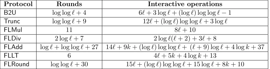
The complexity of this and other protocols in this section are given in Table 1. The numbers listed correspond to the minimal number of rounds and interactive operations, which often requires rearranging computation in the protocols. For example, computing 2[b][v] + (1−[b])[v] on line 4 of
The main component of our division protocol is a simplified divisionSDivgiven in Appendix A, which we modified from the fixed point divisionFPDiv in [17]. Because FPDiv uses Goldschmidt’s method for division, it pays the price of normalizing the divisor in order to compute the initial approximation. With our floating point representation, however, all values are already normalized, and the initial approximation can be computed at very low cost. In fact, since the divisor in our format is between 2`−1 and 2`−1, our initial approximation of one over the divisor is always set to 2−`. We provide additional details aboutSDiv in Appendix A.
As the first step of our floating point division protocolFLDiv, we execute simple divisionSDivon the significands (line 1). Note that, in order to avoid executing it on a zero divisor, we ensure that the second argument to SDiv is non-zero. The output ofSDiv is a normalized either (`+ 1)-bit or
`-bit value. The truncation on line 3 assures that the final value of division is always a normalized
`-bit value. We then adjust the exponent p of the result accordingly. When z2 is set, we need to
also set the error flag (division by 0 if z1 is not set and invalid operation when z1 is also set).
(h[v],[p],[z],[s]i,[Error])←FLDiv(h[v1],[p1],[z1],[s1]i,h[v2],[p2],[z2],[s2]i)
1. [v]←SDiv([v1],[v2] + [z2], `);
2. [b]←LT([v],2`, `+ 1);
3. [v]←Trunc(2[b][v] + (1−[b])[v], `+ 1,1); 4. [p]←(1−[z1])([p1]−[p2]−`+ 1−[b]);
5. [z]←[z1];
6. [s]←XOR([s1],[s2]);
7. [Error]←[z2];
8. return (h[v],[p],[z],[s]i,[Error]);
4.2.2 Addition and subtraction
Addition and subtraction of floating point values is more involved due to the need to align the ar-guments to the same exponents. Also, we do not explicitly provide a subtraction protocol as subtrac-tionFLSub(h[v1],[p1],[z1],[s1]i,h[v2],[p2], [z2],[s2]i) can be performed by callingFLAdd(h[v1],[p1],[z1],
[s1]i,h[v2],[p2],[z2],1−[s2]i).
The intuition behind our approach is to shift the significand of the larger input by the appro-priate number of bits to align the inputs, then perform addition using the inputs’ signs, followed by truncation and normalization.
In the protocol below, we first compute shares of the larger and the smaller of both the signifi-cands and exponents, denoted byvmax,vmin,pmax, andpmin, respectively (lines 1–7). Computation of the exponents is straightforward, while for significands, if the exponents p1 and p2 differ, the
larger value vmax is set based on the summand with the larger exponent, otherwise, it is set based on the larger significand.
The logic used in the protocol depends on the signs of inputs (i.e., if they are the same, the values are being added; otherwise, they are being subtracted), and the differences3(line 8) indicates
which case takes place. We also need to look at the difference between the exponents, denoted by ∆. There are two cases to consider: (i) ∆ > ` and (ii) 0 ≤ ∆ ≤ `. When ∆ > ` and s3 = 0
(addition), there is no need to perform addition and the significand and exponent of the output are set to vmax and pmax, respectively.3 When ∆> ` and s3 = 1 (subtraction), how the algorithm
proceeds depends on whethervmax >2`−1 or otherwisevmax = 2`−1. In the former case, to obtain
3
As with all other protocols, we store the most significant` bits of the result by truncating all remaining bits
the result, we need to subtract 1 from vmax, while setting the exponent topmax. This is because when we subtractvmin fromvmaxthe result will have the same exponent aspmax and its significand will bevmax−1 because we only keep `most significant bits. In the latter case, vmax= 2`−1, and the final result’s significand will be `−1 bits long consisting of all 1s, which we can make ` bits long by appending a 1 and setting the exponent to pmax−1. To accommodate both cases in one statement, we usev3= 2(vmax−s3) + 1 on line 11. If the former case occurs, thenv3 will have`+ 1
bits in which case the extra least significant bit will be later removed. If the latter case occurs,
v3 will contain the correct`-bit value, but the exponent will later need to be set by decrementing
pmax.
When ∆ ≤ `, we keep the minimum exponent and shift the maximum significand by ∆ bits. This is done by multiplying vmax by 2∆, where 2∆ is obtained using Pow2 function (line 10). Therefore v4 =vmax2∆+ (1−2s3)vmin will have `+ ∆±1 bits, which is at most 2`. Next, we combine the two cases above (line 13) using the result of the comparison on line 9: v is either v3
(when ∆> `) orv4 (when ∆≤`). To makev of a fixed length we also multiply it by 2`−∆. Note
that `−∆ is always positive. We obtain that now v will have 2`+δ bits where δ is either 0 or ±1. Because we can only keep `most significant bits of v, we truncate`−1 least significant bits from the result to ensure that at least ` most significant bits of v are always kept (line 14). Now we need to normalize the result and remove the extra bits. To do so, we first bit-decomposev and using prefix-OR calculate the locationp0of the most significant bit set to 1 inv’s bit decomposition
(lines 15–17). Then we shiftv to left byp0 bits by multiplying the value by 2p0. Nowvhas exactly
`+ 2 bits and is normalized, from which two least significant bits are removed (line 18–19). We also need to adjust the exponent of the result to reflect the shiftings and truncations per-formed. If ∆> `, thenp0= 0 when v >2`−1 and p0 = 1 otherwise when v= 2`−1. Thus the final
exponent should be pmax−p0. If ∆≤`, then since we truncate the result by ∆ + 1 and then we
shift it by p0, the original exponent pmin needs to be adjusted accordingly. This means that the final exponent p will bepmin+ ∆ + 1−p0 =pmax−p0+ 1 (line 20).
Lastly, we check whether any of the original summands are 0, in which case the computed sum can be incorrect, and the result instead is set to equal the non-zero summand (line 21).
The rest of the algorithm computes the remaining elements of the result. In particular, the zero bit is set based on whether the computed significand is 0. The exponent is adjusted similar to the adjustment of the significand on line 21 and takes into account zero values. The computation of the sign of the result on line 24 is similar to the computation of the larger significand on line 7 using the sign of the larger summand. The sign is then adjusted (similar tov and p) to take into account zero values (line 25).
h[v],[p],[z],[s]i ←FLAdd(h[v1],[p1],[z1],[s1]i,h[v2],[p2],[z2], [s2]i)
1. [a]←LT([p1],[p2], k);
2. [b]←EQ([p1],[p2], k);
3. [c]←LT([v1],[v2], `);
4. [pmax]←[a][p2] + (1−[a])[p1];
5. [pmin]←(1−[a])[p2] + [a][p1];
6. [vmax]←(1−[b])([a][v2] + (1−[a])[v1]) + [b]([c][v2] + (1−[c])[v1]);
7. [vmin]←(1−[b])([a][v1] + (1−[a])[v2]) + [b]([c][v1] + (1−[c])[v2]);
8. [s3]←XOR([s1],[s2]);
9. [d]←LT(`,[pmax]−[pmin], k);
Protocol Rounds Interactive operations
B2U log log`+ 4 6`+ 3 log`+ (log`) log log`−1
Trunc log log`+ 9 12`+ (log`) log log`+ 3 log`
FLMul 11 8`+ 10
FLDiv 2 log`+ 7 2 log`(`+ 2) + 3`+ 8
FLAdd log`+ log log`+ 27 14`+ 9k+ (log`) log log`+ (`+ 9) log`+ 4 logk+ 37
FLLT 6 4`+ 5k+ 4 logk+ 13
FLRound log log`+ 30 15`+ (log`) log log`+ 15 log`+ 8k+ 10
Table 1: Complexity of floating point and supplemental protocols.
12. [v4]←[vmax][2∆] + (1−2[s3])[vmin];
13. [v]←([d][v3] + (1−[d])[v4])2`Inv([2∆]);
14. [v]←Trunc([v],2`+ 1, `−1);
15. [u`+1], . . . ,[u0]←BitDec([v], `+ 2, `+ 2);
16. [h0], . . . ,[h`+1]←PreOR([u`+1], . . . ,[u0]);
17. [p0]←`+ 2−P`i=0+1[hi];
18. [2p0]←1 +P`+1
i=02i(1−[hi]);
19. [v]←Trunc([2p0][v], `+ 2,2); 20. [p]←[pmax]−[p0] + 1−[d];
21. [v]←(1−[z1])(1−[z2])[v] + [z1][v2] + [z2][v1];
22. [z]←EQZ([v], `);
23. [p]←((1−[z1])(1−[z2])[p] + [z1][p2] + [z2][p1])(1−[z]);
24. [s]←(1−[b])([a][s2] + (1−[a])[s1]) + [b]([c][s2] + (1−[c])[s1]);
25. [s]←(1−[z1])(1−[z2])[s] + (1−[z1])[z2][s1] + [z1](1−[z2])[s2];
26. returnh[v],[p],[z],[s]i;
As in the case of FLMul, complexity of FLAddcan be reduced when one operand is a constant given in the clear. In this case, not only a number of multiplications can be performed locally, but also depending on the operand’s value, some other operations might become unnecessary (e.g., the comparison on line 3).
4.2.3 Additional operations
We conclude description of basic floating point operations by providing two other commonly used operations: comparisons and rounding.
The comparison operation below outputs bit b, which is set to 1 iff the first operand is less than the second operand. Based on the inputs’ signs and zero indicators, their exponents determine which input is larger. When neither of the operands is 0 and they have the same sign, the result can be determined by comparing the exponents (and the significands as well when the exponents are equal). This computation appears on lines 1–5. In the protocol,b+and b− denote the result of comparison if both inputs are positive and if both are negative, respectively. Then line 6 adjusts the result to cover the cases when at least one operand is 0 or when the signs are different ([s1](1−[s2])
is used for opposite signs on line 6). Note that when both inputs are negative with different exponents, the one with the smaller exponent is larger. Also note that when both operands are 0 or equal, the output of this function is 0.
1. [a]←LT([p1],[p2], k);
2. [c]←EQ([p1],[p2], k);
3. [d]←LT((1−2[s1])[v1],(1−2[s2])[v2], `+ 1);
4. [b+]←[c][d] + (1−[c])[a]; 5. [b−]←[c][d] + (1−[c])(1−[a]);
6. [b]←[z1](1−[z2])(1−[s2]) + (1−[z1])[z2][s1] + (1−[z1])(1−[z2])([s1](1−[s2]) + (1−[s1])(1−
[s2])[b+] + [s1][s2][b−]);
7. return [b];
Other relations (such as less than or equal, greater than, equality, etc.) can be easily constructed from the above protocol. It is not difficult to construct FLEQprotocol that avoids calls toLT and is more efficient.
The rounding function FLRound that we provide operates in two different modes: if mode= 0, it computes floor, and ifmode= 1, it computes ceiling.
The logic behind our approach is simple: The input has a fractional part only if its exponent is negative. In this case, we need to truncate the input’s significand to remove only the fractional part.
As the first step of our protocol (lines 1–2), we look at the input’s exponent p1. Ifp1 <−`+ 1,
then the input value is from the range (−1,1) and thus the output should be either 0 or ±1 depending onmode. If, however, p1 is positive, the output of the rounding function is equal to the
input (i.e., the input is an integer). The only case that requires non-trivial computation is when
p1 is between 0 and−`. In this case, rounding amounts to setting −p1 least significant bits of the
significand v1 to 0. Furthermore, if those bits are not all 0, then based on the input’s sign and
mode we need to add 2−p1 to the significand, the effect of which will be incrementing the integer value by 1. For instance, if we are to compute the floor of input −3.54, then the output should be −(3 + 1) =−4. This computation is performed on lines 3–5.
Now, if the addition on line 5 results in an overflow, then the result v needs to be adjusted. Because 2`−1 ≤ v1 < 2` and we are adding either 0 or 1 to it, the overflow happens only when
v= 2`. In this case, we set the value to 2`−1 (line 7) and increment the exponent by 1. To properly set the sign of the output, notice that the sign does not change unless the input belongs to the range (−1,0) and the function computes the ceiling. In those circumstances, we output is 0 and we to set the sign sto 0 as well (line 9). Lastly, we compute the zero bit of the result and adjust the exponent if necessary.
h[v],[p],[z],[s]i ←FLRound(h[v1],[p1],[z1],[s1]i,mode)
1. [a]←LTZ([p1], k);
2. [b]←LT([p1],−`+ 1, k)
3. h[v2],[2−p1]i ←Mod2m([v1], `,−[a](1−[b])[p1]);
4. [c]←EQZ([v2], `);
5. [v]←[v1]−[v2] + (1−[c])[2−p1](XOR(mode,[s1]));
6. [d]←EQ([v],2`, `+ 1); 7. [v]←[d]2`−1+ (1−[d])[v];
8. [v]←[a]((1−[b])[v] + [b](mode−[s1])) + (1−[a])[v1];
9. [s]←(1−[b]mode)[s1];
10. [z]←OR(EQZ([v], `),[z1]);
11. [v]←[v](1−[z]);
12. [p]←([p1] + [d][a](1−[b]))(1−[z]);
Above we use a slightly modified Mod2m([a], `,[m]), which in addition to computing [amod 2m] also outputs [2m], which is computed a part of the protocol. This allows us to avoid redundancy in computing [2−p1].
We also note that our rounding functionality can be easily realized when mode is secret-shared. This allows the parties to execute input-based rounding operations. Furthermore, round-ing to the nearest integer FLRound(h[v1],[p1],[z1],[s1]i,mode = 2) can be achieved by first adding
0.5 in the floating point representation to the input and then executing the floor function (i.e.,
FLRound(FLAdd(h[2`−1],[−`],0,0i,h[v1], [p1],[z1],[s1]i),0)).
5
Type Conversions
In this section we provide methods to convert a value from one representation (i.e., floating point, fixed point, or integer) to another. We use ` and k to denote bitlengths of significands and expo-nents, respectively, in a floating point representation. We also useγ to denote is the total bitlength of values in either integer or fixed point representation, and f to denote the bitlength of the frac-tional part in fixed point values (in other words, fixed point representation uses γ bits, from which
f bits are dedicated to the fractional and γ−f bits are dedicated to the integer part). Note that if x is represented as a fixed point value, then x = x2−f, where x ∈ Zhγi. Thus representing |x| requiresγ−1 bits. Similarly, integer valuesx∈Zhγihave|x|<2γ−1. Although the publicly known bitlengths`, k, γ, f can be passed to protocols, we assume thatk >max(dlog(`+f)e,dlog(γ)e) and the modulusq >max(22`,2γ,2k).
Integer to floating point number. The first protocol that we provide converts a signed γ-bit
integerainto a floating point value, and is given next. It proceeds by first determining the sign of theγ-bit input, normalizes the input, and then fits it into an`-bit representation.
In the protocol, we first determine whether the input is 0 or is negative (lines 2 and 3 below) and turn a into a positive value on line 4. Because we need to normalize the value of a, we bit-decompose it into λ = γ−1 bits (recall that one bit of its γ-bit representation was used for the sign). Prefix OR on line 6 allows us to compute the number of 0 bits in a starting from the most significant bit until the first 1 is observed. If the number of such bits is k, then our goal is to compute normalized value 2ka. We note that by using prefix OR, we set all bits after the most significant 1. Thus, if we flip all bits (i.e., 1−bi), we have k 1s and the rest of bits become 0. Now if we compose all the bits as P
2i(1−bi), we obtain 2k−1. This computation and the final multiplication (a2k) occur on line 7. The output’s exponent needs to be set to−k (line 8) sincea
is now shifted ktimes to the left.
What remains is to represent the value as an `-bit number instead of using λ=γ −1 bits and adjust the exponent accordingly. Therefore, if γ−1> `, we select` most significant bits (line 9); otherwise, we shift the value by`−γ+ 1 to the left to ensure that its most significant bit is 1 (line 10). The exponent is adjusted by the amount of shift on line 11 and reset to 0 if necessary.
h[v],[p],[z],[s]i ←Int2FL([a], γ, `)
1. λ←γ−1; 2. [s]←LTZ([a], γ); 3. [z]←EQZ([a], γ); 4. [a]←(1−2[s])[a];
5. [aλ−1], . . . ,[a0]←BitDec([a], λ, λ);
7. [v]←[a](1 +Pλ−1
i=0 2i(1−[bi])); 8. [p]← −(λ−Pλ−1
i=0[bi]);
9. if (γ−1)> `then [v]←Trunc([v], γ−1, γ−`−1); 10. else [v]←2`−γ+1[v];
11. [p]←([p] +γ−1−`)(1−[z]); 12. returnh[v],[p],[z],[s]i;
Floating point number to integer. Our next protocol converts a floating point input with an
`-bit significand to the nearest integer representable inγ bits. Our approach is to round the input to the nearest integer and then, based on the exponent of the outcome, fit the result into a γ-bit representation.
As a first step in our solution, we round the input to the nearest integer using FLRound with the result still being in the floating point format. The resulting integer can be represented using
`+p0 bits (plus the sign), where p0 is the exponent of the output, and our goal is to produce an
γ-bit signed integer.
We divide all possible options into the following categories: If p0 ≥γ−1, the input is too large to be represented using γ bits. In other words, its last p0 ≥ γ −1 bits are 0 and we output 0. This condition is checked on line 2 of our protocol, but setting the output to 0 is deferred until the end (this allows us not to worry about this case for most of the computation). Otherwise, if
p0+` > γ−1, the value is still too large to be represented usingγ−1 bits, and we have to truncate
`+p0−(γ−1) most significant bits from the significand v0. In other words, the integer will consist of γ −1−p0 least significant bits of v0 followed by p0 0 bits. This condition is checked on line 3. Now, if p0 <0, some of the significand’s bits correspond to the fractional part (while being set to 0) and we need to truncate v0 by p0 bits. This condition is checked on line 4. When p0 < 0, we, however, can still have that p0+` > γ−1 (namely, when ` is much larger than γ), which means that a number of most significant bits of v0 need to be truncated. Assuming that p0 < γ−1 we thus obtain four different cases based on conditionsp0>0 andp0+` > γ−1.
The computation that follows treats the cases above. When 0< p0 < γ−1 and p0+` > γ−1, we keepγ−1−p0 least significant bits of v0 and otherwise keep v0 unchanged (lines 5–7) (note that 1−b−bc is the complement ofb(1−c)). The next 5 lines treat the cases when p0 is negative. In particular, on lines 8–10, we remove p0 least significant bits ofv0 (which are all 0) ifp0 is negative and keepv0 unchanged otherwise. Also,p0 <0 andp0+` > γ−1, we keep onlyγ−1 least significant bits of the output (lines 11–12). What remains is to append p0 0 bits for positive p0, include the sign, and set the value to 0 if necessary.
As an important performance issue, we note that two calls to Mod2m can be combined into a single call and, similarly, two calls toPow2in the protocol can be combined into one, thus noticeably improving the complexity of the algorithm. This is possible because either function is called on mutually exclusive arguments on two occasions (i.e., multiplied by bit c in one case and by bit 1−c in the other), and the result can be updated as before. For readability of this work we do not include them in the protocol.
[g]←FL2Int(h[v],[p],[z],[s]i, `, k, γ)
1. h[v0],[p0],[z0],[s0]i ←FLRound(h[v],[p],[z],[s]i,2); 2. [a]←LT([p0], γ−1, k);
3. [b]←LT(γ−`−1,[p0], k); 4. [c]←LTZ([p0], k);
6. [u]←Mod2m([v0], `,[m]);
7. [v0]←[b](1−[c])[u] + (1−[b] + [b][c])[v0]; 8. [2−p0]←Pow2(−[c][p0], `);
9. [2p0]←Inv([2−p0]);
10. [v0]←([c][2p0] + 1−[c])[v0]; 11. [w]←Mod2m([v0], `,[b][c](γ−1)); 12. [v0]←[b][c][w] + (1−[b][c])[v0]; 13. [2p0]←Pow2([a](1−[c])[p0], γ−1); 14. [g]←(1−[z0])(1−2[s0])[2p0][a][v0]; 15. return [g];
Fixed point to floating point numbers. We next describe a protocol that converts a value
g·2−f in fixed point notation to a floating point representation. We have that g is a signed γ-bit integer, and the resulting floating point number has a `-bit significand and k-bit exponent. To perform the conversion, we call our integer-to-floating-point function Int2FL on the integer g and subtract f from the exponent of the output.
h[v],[p],[z],[s]i ←FP2FL([g], γ, f, `, k)
1. h[v],[p],[z],[s]i ←Int2FL([g], γ, `); 2. [p]←([p]−f)(1−[z]);
3. returnh[v],[p],[z],[s]i;
Floating point to fixed point numbers. Our last protocol converts a floating point number
with a`-bit significand andk-bit exponent to to a fixed point number represented usingγ bits with precision 2−f. This is achieved by converting the input to a γ-bit integer after adding the fixed point precision to the exponent. Note that if the input’s exponent is close enough to the maximum so that if it overflows when f is added to it, the output should be set to zero.
[g]←FL2FP(h[v],[p],[z],[s]i, `, k, γ, f)
1. [b]←LT([p],2k−1−f, k);
2. [g]←FL2Int(h[v],[p] +f,[z],[s]i, `, k, γ)[b]; 3. return [g];
6
Complex Operations
We next present several complex operations on numeric data types. While the approach we take is suitable for secure processing of different data representations, our protocols focus on floating point numbers.
6.1 Square root
As the first operation, we compute x = √y for any positive real number y. To achieve this, one method is to use the old Babylonian formula that has very fast convergence rate
xi+1=
1 2
xi+
y xi
where the initial point x0 is always set to 1. The rate of convergence in this method is quadratic
in the size of the input, which means that the number of bits of accuracy roughly doubles on each iteration. Then, if the precision is`bits, the number of iterations isdlog`e+ 1. As evident from the formula, this method requires one division, one addition, and one multiplication in each iteration. Because division is an expensive operation, there are other methods to approximate√xusing only multiplication and addition with the same rate of logarithmic convergence. One of these methods is Newton-Raphson’s method. As described in [34], this method tries to iteratively approximate the roots of a continuous and at least one time differentiable function. We can apply Newton-Raphson’s method to the functionf(R) = R12 −x to approximate √1x and ultimately approximate
√
xby multiplying the approximation of √1
x by x. The iterative equation in this method is
Ri+1 =
1
2Ri(3−xR
2
i) (1)
This method requires three multiplications and one addition inside the iterative equation. All these operations have to be executed sequentially, thus the round complexity is high.
The most efficient (both in terms of round and communication complexity) approach for com-puting the square root of a positive number is to use the iterative method of Goldschmidt [28]. It provides an approximation of both √x and √1
x with quadratic convergence. This method, as shown in [34], needs an initial approximation of √1
x (denoted by y0) that satisfies 0.5< xy
2 0 <1.5.
The value of y0 is usually approximated using a linear equation y0 = αx+β, where α and β are
predetermined constants that can be found in [34]. Then, ifg is an approximation of √x and h is an approximation of 2√1
x, the iterative equations are:
gi+1 =gi(1.5−gihi) hi+1 =hi(1.5−gihi)
whereh0=y0/2 andg0 =xy0. One of the advantages of this approach is that since gi+1 and hi+1
can be computed in parallel (independently) aftergihi has been computed, the round complexity is reduced (as opposed to Newton-Raphson’s method discussed above). This method is not self-correcting and the error can accumulate. To eliminate the accumulated errors, we take advantage of the self-correcting Newton-Raphson’s approximation method and replace the last iteration of Goldschmidt’s method with one iteration of Newton-Raphson’s method. By replacing Ri/2 with
hi in equation 1, we obtain hi+1 = hi(3/2−2xh2i) as the new formula for approximating 2√1x. Ultimately, at the end of iterations, we need to multiply the last computed hi by 2x to obtain an approximation for√x.
We next provide a protocol that implements Goldschmidt’s approximation (similar to the fixed point protocol of [34]) for the floating point representation. In our representation, the significand of the input 2`−1 ≤v <2` is already normalized and therefore 1/2≤x=v2−` <1. In fact, if we are to calculate the square root ofu=v·2p, we can run our approximation on u=v2−`2p+`=x2p+`. Furthermore,√u=√ax2b(p+`)/2c, whereais either 1 (whenp+`is even) or 2 (whenp+`is odd). In the protocol, we first determine whetherp+`is even or odd (lines 1–2) and set the final exponent tob(p+`)/2c (line 3). Here`0 denotes the least significant bit of `. Next, we compute the initial
approximationy0 using the linear equation mentioned above (lines 4–5). We usehvα, pα, zα, sαiand hvβ, pβ, zβ, sβito denote the floating point representation of α andβ, respectively. The value ofg0
is computed on line 6 by multiplying xby the approximation of √1
x. To computeh0, we only need to subtract 1 from the exponent of y0 (line 7). In the loop (lines 8–12) we follow Goldschmidt’s
that it is not necessary to compute line 11 in the last iteration of Goldschmidt’s algorithm since
gi is not used after the loop. Finally, we need to multiply the result by the factor √
a above to obtain √v (line 18). In the protocol, v√
2 is the `-bit significand of
√
2 and p√
2 is its exponent in
the floating point representation. Our floating point implementation of approximating square root has a substantially smaller complexity than the fixed point protocol of [34] for the same precision. This is due to the fact that in [34] quadratic communication complexity is used to normalize the input while the input in our floating point representation is already normalized.
(h[v],[p],[z],[s]i,[Error])←FLSqrt(h[v1],[p1],[z1],[s1]i)
1. [b]←BitDec([p1], `,1);
2. [c]←XOR([b], `0);
3. [p]←([p1]−[b])2−1+b`/2c+OR([b], `0);
4. h[v2],[p2],[z2],[s2]i ←FLMul(h[v1],−`,0,0i,hvα, pα,zα, sαi); 5. h[v0],[p0],[z0],[s0]i ←FLAdd(h[v2],[p2],[z2],[s2]i,hvβ,pβ, zβ, sβi); 6. h[vg],[pg],[zg],[sg]i ←FLMul(h[v1],−`,0,0i,h[v0],[p0], [z0],[s0]i);
7. h[vh],[ph],[zh],[sh]i ← h[v0],[p0]−1,[z0],[s0]i;
8. fori= 1 to dlog(`/5.4)e −1
9. h[v2],[p2],[z2],[s2]i ←FLMul(h[vg],[pg],[zg],[sg]i,h[vh],[ph],[zh],[sh]i); 10. h[v2],[p2],[z2],[s2]i ←FLSub(h3·2`−2,−(`−1),0, 0i,h[v2],[p2],[z2],[s2]i);
11. h[vg],[pg],[zg],[sg]i ←FLMul(h[vg],[pg],[zg],[sg]i,h[v2],[p2],[z2],[s2]i);
12. h[vh],[ph],[zh],[sh]i ←FLMul(h[vh],[ph],[zh],[sh]i ,h[v2],[p2],[z2],[s2]i);
13. h[vh2],[ph2],[zh2],[sh2]i ←FLMul(h[vh],[ph],[zh],[sh]i,h[vh],[ph],[zh],[sh]i); 14. h[v2],[p2],[z2],[s2]i ←FLMul(h[v1],−`,0,0i,h[vh2], [ph2],[zh2],[sh2]i);
15. h[v2],[p2],[z2],[s2]i ←FLSub(h3·2`−2,−(`−1),0,0i,h[v2],[p2] + 1,[z2],[s2]i);
16. h[vh],[ph],[zh],[sh]i ←FLMul(h[vh],[ph],[zh],[sh]i,h[v2],[p2],[z2],[s2]i);
17. h[v2],[p2],[z2],[s2]i ←FLMul(h[v1],−`,0,0i,h[vh], [ph] + 1,[zh],[sh]i);
18. h[v2],[p2],[z2],[s2]i ← FLMul(h[v2],[p2],[z2],[s2]i, h(1−[c])2`−1 + [c]v√2,−(1−[c])(`−1) +
[c]p√
2,0,0i);
19. [p]←([p2] + [p])(1−[z1]);
20. [v]←[v2](1−[z1]);
21. [Error]←[s1];
22. return (h[v],[p],[z1],[s1]i,[Error]);
6.2 Exponentiation
We next treat exponentiation for the case that when the base is 2. Recall that exponentiation with an arbitrary base b can be computed as ba = 2alogb, and we subsequently provide a solution for computing logb when b is a floating point number. In our solution below we try to avoid any use of series since floating point addition is quite expensive. In fact, out approach does not rely on any floating point operations introduced above.
As any real number has an integer and fractional parts (e.g., 11001.01011), when 2 is raised to the power of that number, we break it into two components: 2 to the power of the integer part (in this example 211001) times 2 to the power of fractional part (20.01011). In fact, if we have the
fractional part in a bit decomposed formu1,· · ·, un, we can compute
20.u1···un =Yn
i=12
ui2−i =Yn
i=1(ui2 2−i
+ (1−ui)) (2)
i=`. We therefore use a set of floating point constants 22−i fori= 1, . . ., `. The above intuition leads toFLExp2 protocol for computing exponentiation on a secret-shared floating point exponent that we describe next.
Given a floating point input, we would like to represent it asw.u, wherewanduare the integer and fractional parts, respectively. We only need to consider the ` most significant bits of u to achieve our desired precision. The computation that we perform to produce the integer w and fractional u parts depends on the sign of the input, since we demand the fractional part to be positive. Therefore, in some cases we may need to subtract 1 from the integer part to guarantee that the fractional part is positive, but regardless of the input, the output of the exponentiation will be 2w multiplied by 20.u. We follow the approach above to compute 20.u using bit decomposition.
To determinewandu, we divide the range of the input’s exponentp1(for non-zero inputs) into
four regions: (i) whenp1≤ −2`(i.e., the value is so small that effectivelyw= 0 andu= 0), (ii) when
−2` < p1 ≤ −` (i.e., the input can occupy only the fractional part u), (iii) when −` < p1 ≤max
(i.e.,w6= 0 andu6= 0), and (iv) whenmax < p1(i.e., the input is too large and results in an overflow
or underflow). Heremaxrepresents the value exceeding which for the exponent guarantees either an overflow (for a positive input) or underflow (for a negative input) in the output of the function. We compute it as follows: the maximum value that we can represent is (2`−1)22k−1−1. An overflow for this function occurs whenever 2v1·2p1
exceeds that value for a positive input with significandv1 and
exponentp1. Becausev1 ≥2`−1, an overflow is guaranteed when 22
`−12p1
>(2`−1)22k−1−1, which allows us to compute the maximum value p1 can take. The same reasoning applies to underflow
for negative inputs. Note the the purpose of max is not to detect all possible cases of overflow and underflow (which should be done at the end of the computation if error checking is used), but rather ensure correct operation of the protocol. Thus, in our protocol FLExp2 we first compute thismax value and proceed with processing all four regions in parallel. We first provide a protocol that works in the most common case of` > k (max <0). We then modify our protocol slightly to address all cases of `and k.
The region in which the input falls is determined using three comparisons on lines 2–4. Let us first consider the third region with −` < p1 ≤ max, which corresponds to values a = 1, b = 0,
and c = 0 in the protocol. In this case, the input has non-zero integer and fractional parts. We know that the integer part is the truncation of v1 by p2 = −p1 and thus we separate the integer
and fractional parts and store them in variables x and y, respectively (lines 5–7). To use the bit-decomposition idea above, we need to make sure that the fractional part u that will be bit-decomposed is always positive. In this region it can be negative if after the initial computation on line 7 its value is non-zero and the input is negative. Thus, when both conditions are true, we subtract 1 from the integer part (i.e., w = x−1) and subtract the fractional part from 1 (i.e., 0.u = 1−0.y). To accomplish this in the protocol, we first test whether y 6= 0 (line 8), subtract 1 from x when s1 = 1 and y 6= 0 (line 9), and subtract y from 2p2 when s1 = 1 and y 6= 0 (line
10). For inputs in this region (with a= 1, b= 0, and c= 0) we keepw unchanged on line 11, but normalize uon line 12.
If the input falls into the second region with −2` < p1 ≤ −`, we have that a= 1, b= 1, and
c= 0. In this case, the input is too small to contain any integer part (i.e., the integer partw is 0), and we need to compute only the fractional part. In this case, we truncate the input’s significand by p2 =−(p1+`) and store the result, which now represents the fractional part, inx (lines 5–6).
Because we only keep`most significant bits of the fractional part, in this region we can throw away the leftover of the truncation (i.e., y is not used). If the input is positive, we will have w= 0 and
from 2`. Furthermore, because our protocols round down, for negative inputs we setx= 2`−x−1 ify 6= 0 and x = 2`−x otherwise. In the protocol, this computation is performed on lines 9 and 11, andu is set tox on line 12 (witha= 1, b= 1, andc= 0).
If the input falls into the first region, we have p1 ≤ −2` and a= 1, b = 1, and c= 1 on lines
2–4. In this case, we consider two sub-cases based on the sign of the input. In this region the input is too small to be representable with`-bit precision and when the input is positive (i.e.,s1 = 0), we
set the output to 20= 1. If the input is negative, we need to make the fractional part positive. We accomplish this by setting the integer part of the input to −1 and subtracting the fractional part from 1. Because we only keep the first`bits of the fractional part, for this region all bits will be 1 for non-zero inputs because rounding down is used and we can set u= 2`−1. In our protocol this computation is accomplished on lines 11 and 12 (witha=b=c= 1), i.e., x andy are not used.
Lastly, if the input falls into the fourth region, we have max < p1 and a=b =c= 0. In this
case, the output’s exponent will be too large and outside of the representable range, which means that we have an error. To address this, we set w and u to 0 on lines 11 and 12. At the end of the protocol, we set the exponent to 2k−1 (or −2k−1 for negative inputs), which is outside of the representable range to indicate an overflow or underflow.
The loop on lines 14–16 computes the terms in the product in equation 2. We use constants hcvi, cpi,0,0i to represent 22
−i
in the floating point format, and thus ai and bi correspond to the significand and exponent of (ui22−i+ (1−ui)), respectively. Multiplication of all of these terms is accomplished on line 17. The notationFLProddenotes the computation of the product of a number of floating point values. Instead of` sequential multiplications in our case, it can be implemented indlog`e rounds by constructing a tree of pairwise multiplications (i.e., `/2 multiplications at the lowest level, `/4 multiplications at the next level, etc.). With the availability of constant round prefix multiplication for floating point numbers, the round complexity of this operation could be reduced to constant rounds. We leave this as a direction for future work.
After computing the product as in equation 2, we multiply the result by 2w, which is performed on line 18 by increasing the exponent of the result by w. On line 18 we also set the exponent to a value outside of the representable range for inputs falling into the fourth region (with a= 0) to indicate an overflow or underflow.
Finally, the remainder of the protocol (lines 19–20) addresses the case when the input is 0 and sets the result to be 1 in the normalized form (i.e., with v= 2`−1 and p=−(`−1)).
h[v],[p],[z],[s]i ←FLExp2(h[v1],[p1],[z1],[s1]i)
1. max←
log(2k−1−1 +`)−`+ 1; 2. [a]←LT([p1], max, k);
3. [b]←LT([p1],−`+ 1, k);
4. [c]←LT([p1],−2`+ 1, k);
5. [p2]← −[a](1−[c])([b]([p1] +`) + (1−[b])[p1])
6. h[x],[2p2]i ←Trunc([v
1], `,[p2]);
7. [y]←[v1]−[x][2p2];
8. [d]←EQZ([y], `);
9. [x]←(1−[b][s1])([x]−(1−[d])[s1]) + [b][s1](2`−1 + [d]−[x]);
10. [y]←(1−[d])[s1]([2p2]−[y]) + (1−[s1])[y];
11. [w]←[a](1−[c])((1−[b])[x] + [b][s1])(1−2[s1])−[c][s1];
12. [u]←[a](1−[c])([b][x] + (1−[b])(2`·Inv([2p2]))[y]) + (2`−1)[c][s
1];
13. [u`], . . . ,[u1]←BitDec([u], `, `);
15. [ai]←2`−1(1−[ui]) + (cvi)[ui]; 16. [bi]← −(`−1)(1−[ui]) + (cpi)[ui];
17. h[vu],[pu],0,0i ←FLProd(h[a1],[b1],0,0i, . . .,h[a`],[b`], 0,0i);
18. [p]←[a]([w] + [pu]) + 2k−1(1−[a])(1−2[s1]);
19. [v]←2`−1[z1] + (1−[z1])[vu]; 20. [p]← −[z1](`−1) + (1−[z1])[p];
21. returnh[v],[p],[0],[0]i;
The protocol above works under the assumption thatk < `, which is normally the case as mentioned above. If, however, it is desirable to usek≥`, we provide a modified (and slightly more expensive) solution below. This modified protocol is similar to the one presented above, and the differences are specific to handling exponents longer than significands. From all four regions of the exponents, only the third region is affected in which case p1 may be positive (since max > 0 when k ≥ `).
In this protocol, lines 6, 7, and 14 are new, and line 6 tests whether the value of p2, by which
the significand is to be truncated, is negative. The result of this comparison is used on line 8 to guarantee that the truncation is always performed by a non-negative amount and on line 14 to normalize the value by shifting it if p1 is positive. Positive exponent p1 that falls into the third
region will result in an overflow or underflow.
h[v],[p],[z],[s]i ←FLExp2(h[v1],[p1],[z1],[s1]i)
1. max←
log(2k−1−1 +`)−`+ 1
; 2. [a]←LT([p1], max, k);
3. [b]←LT([p1],−`+ 1, k);
4. [c]←LT([p1],−2`+ 1, k);
5. [p2]← −[a](1−[c])([b]([p1] +`) + (1−[b])[p1])
6. [e]←LTZ([p2], k);
7. [2p1]←Pow2([e][p
1],2k−`+ 1);
8. h[x],[2p2]i ←Trunc([v
1], `,(1−[e])[p2]);
9. [y]←[v1]−[x][2p2];
10. [d]←EQZ([y], `);
11. [x]←(1−[b][s1])([x]−(1−[d])[s1]) + [b][s1](2`−1 + [d]−[x]);
12. [y]←(1−[d])[s1]([2p2]−[y]) + (1−[s1])[y];
13. [w]←[a](1−[c])((1−[b])[x] + [b][s1])(1−2[s1])−[c][s1];
14. [w]←(1−[e])[w] + [e](1−2[s1])[v1][2p1];
15. [u]←[a](1−[c])([b][x] + (1−[b])(2`·Inv([2p2]))[y]) + (2`−1)[c][s
1];
16. [u`], . . . ,[u1]←BitDec([u], `, `);
17. fori= 1 to `do in parallel 18. [ai]←2`−1(1−[ui]) + (cvi)[ui]; 19. [bi]← −(`−1)(1−[ui]) + (cpi)[ui];
20. h[vu],[pu],0,0i ←FLProd(h[a1],[b1],0,0i, . . .,h[a`],[b`], 0,0i);
21. [p]←[a]([w] + [pu]) + 2k−1(1−[a])(1−2[s1]);
22. [v]←(1−[z1])[vu] + 2`−1[z1];
23. [p]←(1−[z1])[p]−(`−1)[z1];
6.3 Logarithm
The last operation that we present is computing logarithm to the base 2. Recall that for other bases b the function can be computed as logb(x) = log2(x)/log2(b). In the following description, we useeto represent the Euler’s constant.
To compute the logarithm of a positive number in any representation, we can utilize the formula
logx= 2 logearctanx−1
x+ 1
and approximate arctanx by bounding its Taylor’s series as arctanx ≈ PM
i=0 x
2i+1
(2i+1) for |x| < 1.
This gives us
logx≈2 loge
M
X
i=0
z2i+1
(2i+ 1),
wherez= xx−+11. In general, z≤zmax = xxmaxmax−+11, wherexmax is the maximum value of inputx, and to achieve `-bit precision, we need to useM >d`/(−2 logzmax)−1/2e. For practical values of `, this approach finishes faster than using Taylor’s series, since not only the latter approach requires more interactive rounds of computation but also finding the initial approximation is not trivial.
In our floating point representation, a positive value is represented as x=v·2p, where 2`−1 ≤
v < 2`. We can therefore write v as 2`u where 1/2 ≤ u < 1 −2−`. In this representation, logx=`+p+ logu, and we use the above approximation to derive the formula:
logx=`+p− M
X
i=0
2 logey
2i+1
2i+ 1 (3)
wherey= (1−v2−`)/(1 +v2−`). This computation requires one division, 2(M+ 1) multiplications, and M + 2 additions, where M =d`/(2 log 3)−1/2e to achieve ` bits of precision. Note that one can apply Pad´e approximants [10] to the Taylor’s series above to reduce the round complexity at the cost of (noticeably) increasing the communication complexity of the protocol. We omit the details of such a technique.
Throughout most of our protocol FLLog2below for computing the logarithm of floating point values, we assume that the input is positive. If the input is either 0 (the log of which is −∞, division by zero exception) or negative (the log of which is a complex number, invalid operation exception), the error flag will be set (line 16).
The first 3 lines of the protocol compute y = (1−v12−`)/(1 +v12−`) in the floating point
notation, followed by the computation ofy2 on line 4. Because the powers ofy in the series above are all odd, in each iteration, we multiply the previousy2(i−1)+1byy2to obtainy2i+1(line 9). In the protocol, we use constantshcvi, cpi,0,0ifori= 0, . . ., M to denote the floating point representation of (22 logi+1)e. The variable (v, p) holds the current value of the sum in equation 3 (initialized on line 5 to the 0th constant times y) and the variable (vy, py) holds the current power ofy. (The variables with subscripts 2 and 3 hold intermediate results.) Then inside the loop we update the current power ofy, multiply it by the appropriate constant, and add the result to the sum (lines 7–9).
After exiting the loop, we need to subtract the computed sum from p+`. To do so, we first convert p+` into the floating point format (line 10) and then perform the subtraction (line 11) to obtain the final result. The rest of the function sets the output to 0 in case the input was 1 (represented ash2`−1,−(`−1),0,0i) and performs error checking.
1. h[v2],[p2],0,0i ←FLSub(h2`−1,−(`−1),0,0i,h[v1], −`,0,0i);
2. h[v3],[p3],0,0i ←FLAdd(h2`−1,−(`−1),0,0i,h[v1], −`,0,0i);
3. (h[vy],[py],0,0i,0)←FLDiv(h[v2],[p2],0,0i,h[v3],[p3], 0,0);
4. h[vy2],[py2],0,0i ←FLMul(h[vy],[py],0,0i,h[vy],[py],0, 0i); 5. h[v],[p],0,0i ←FLMul(h[vy],[py],0,0i,hcv0, cp0,0,0i);
6. fori= 1 to M do in parallel
7. h[vy],[py],0,0i ←FLMul(h[vy],[py],0,0i,h[vy2],[py2], 0,0i); 8. h[v2],[p2],0,0i ←FLMul(h[vy],[py],0,0i,hcvi, cpi,0, 0i); 9. h[v],[p],0,0i ←FLAdd(h[v],[p],0,0i,h[v2],[p2],0,0i);
10. h[v2],[p2],[z2],[s2]i ←Int2FL(`−[p], `, `);
11. h[v],[p],[z],[s]i ←FLSub(h[v2],[p2],[z2],[s2]i,h[v],[p],0, 0i);
12. [a]←EQ([p1],−(`−1), k);
13. [b]←EQ([v1],2`−1, `);
14. [z]←[a][b]; 15. [v]←[v](1−[z]); 16. [Error]←OR([z1],[s1]);
17. [p]←[p](1−[z]);
18. return (h[v],[p],[z],[s]i,[Error]);
7
Security Analysis
Correctness of the computation has been discussed with each respective protocol, and we now proceed with showing their security.
First, we note that the linear secret sharing scheme achieves perfect secrecy in presence of collusions of size at mostt (i.e., no information can be learned about secret-shared values by tor fewer parties) in the case of passive adversaries. Similarly, the multiplication protocol does not reveal any information, as the only information transmitted to the participants are the shares. Furthermore, because other building blocks used in this work (e.g., EQ, PreMul, etc.) have been previously shown to be secure, information is not revealed during their execution as well. The only value that is revealed in all of our protocols is c inB2U and Trunc. It, however, statistically hides any sensitive information, and the parties will not be able to learn any information about private values with non-negligible probability. We obtain that our protocols combine only secure building blocks without revealing any information to the computational parties. By Cannetti’s composition theorem [14], we have that composition of secure sub-protocols results in security of the overall solution. More formally, to comply with the security definition, we can build a simulator for our protocols by invoking simulators for the corresponding building blocks to result in the environment that will be indistinguishable from the real protocol execution by the participants.
among the participants (when the dealer is dishonest) and proofs of proper reconstruction of a value from its shares (when not already implied by other techniques). In addition, if at any point of the computation the participants are required to input values of a specific form, they would have to prove that the values they supplied are well formed. Such proofs are not necessary for the computation that we use to construct our protocols, but are needed by the implementations of some of the building blocks (e.g.,RandInt).
Thus, security of our protocols in the malicious model can be achieved by using standard VSS techniques, e.g., [27, 18], where a range proof, e.g., [37] will be additionally needed for the building blocks. These VSS techniques would also work with malicious input parties (who distribute inputs among the computational parties), who would need to prove that they generate legitimate shares of their data.
8
Experimental Results
In order to compare performance of arithmetic using different data types, we implement functions for integer, fixed point, and floating point operations. All implemented floating point operations — namely, multiplication (FLMul), division (FLDiv), addition (FLAdd), comparison (FLLT), exponen-tiation (FLExp2), and logarithm (FLLog2) — were tested for correctness. The tests were designed to cover special cases of relevance to the protocols. In particular, inputs to all of the above functions were formed using each combination from the following list:
• significand: 2`−1, 2`−1+ 1, 2`−1
• exponent: 0,−`, +`,−2`, +2`, and a low positive constant • sign bit: 0, 1
• zero bit: 0, 1
This gives 37 possibilities for each operand. In addition, for the exponentiation we used additional tests specific to the implementation of that function, which divides all inputs into four regions. In particular, we add tests with exponents equal to −2`+ 1, −`+ 1,max−1, andmax.
In the experiments, for floating point values we use bitlengths`= 32 for significands andk= 9 for (signed) exponents. This allows us to represent real values with precision 2−256. For (signed) fixed point representation, we use bitlength γ = 64 with f = 32 (i.e., 32 bits before and after the radix point). This gives us precision 2−32 while covering values with the integer part up to 31 bits. Lastly, for (signed) integer computation we use length γ = 64, which makes it easier to compare performance with that of fixed point values (recall that a fixed point value g is represented as integerg·2f).
We set statistical hiding parameter κ= 48 for all data types. For integer arithmetic, the size of the field is determined by the bitlengths necessary for division and we obtain|q|>2γ+κ+ 1 = 177 (if division is known to not be used, the field size can be reduced to use |q|> γ+κ = 112). For fixed point arithmetic, the field size is also determined by the length of the values used during division and we obtain |q|> γ+ 3f +κ = 208 (once again, if division is not used, the size of the field can be reduced to use|q|> γ+f+κ= 144). Lastly, for floating point arithmetic, we need to have |q|>2`+κ+ 1 = 113.