The Measurement Of Efficiency Where There Are Multiple Outputs

Full text

(1)CENTRE of POLICY STUDIESand the IMPACT PROJECT. Eleventh Floor Menzies Building Monash University Wellington Road CLAYTON Vic 3800 AUSTRALIA Telephone: (03) 9905 2398, (03) 9905 5112. from overseas: 61 3 9905 2398 61 3 9905 5112 61 3 9905 2426. Fax : (03) 9905 2426 e-mail web site:. [email protected] http://www.monash.edu.au/policy/. T HE M EASUREMENT OF EFFICIENCY WHERE THERE ARE M ULTIPLE O UTPUTS by. John L. WHITEMAN. Centre of Policy Studies, Monash University. General Paper No. G-134 November 1999. ISSN 1031 9034. ISBN 0 7326 1519 4. The Centre of Policy Studies is a research centre at Monash University devoted to quantitative analysis of issues relevant to Australian economic policy..

(2) The Measurement of Efficiency where there are Multiple Outputs. Abstract This paper is motivated by the empirical observation that in many studies the elasticity of output with respect to labour is often negative and/or insignificant. The present study applies multiple output models to estimate the technical efficiency of enterprises in the international electricity, gas and telecommunications industries. The results support the contention that single output production models may yield misleading results in respect of the elasticities of inputs such as labour. The results also suggest that relatively simple DEA and ordinary least squares models may be preferred to more complex stochastic frontier models in estimating the technical efficiency of enterprises.. Journal of Economic Literature Classification Numbers: D24, L94, L95, L96.. Keywords: multiple output, data envelopment analysis, stochastic production frontier, distance function, ray frontier, technical efficiency.. i.

(3) CONTENTS Page Abstract. i. 1.. Introduction. 1. 2.. Data Envelopment Analysis (DEA). 2. 3.. Multi-output distance functions. 2. 4.. Multiple output ray frontier production model. 4. 5.. Data. 6. 6.. Results. 7. 7.. Summary and conclusions. 10. References. 12. List of Tables 1.. Summary of data on electricity suppliers. 14. 2.. Summary of data on gas suppliers. 15. 3.. Summary of data on telecommunications suppliers. 17. 4.. Estimated parameters for alternative models: Electricity. 18. 5.. Estimated parameters for alternative models: Gas. 19. 6.. Estimated parameters for alternative models: Telecommunications. 20. 7.. Technical efficiency for alternative models: Electricity. 21. 8.. Technical efficiency for alternative models: Gas. 22. 9.. Technical efficiency for alternative models: Telecommunications. 24. 10. Correlation table of alternative technical efficiency measures: Electricity. 25. 11. Correlation table of alternative technical efficiency measures: Electricity. 25. 12. Correlation table of alternative technical efficiency measures: Electricity. 26. ii.

(4) The Measurement of Efficiency where there are Multiple Outputs. 1. Introduction Single output data envelopment analysis (DEA) and stochastic production frontier (SPF) models are now being used more and more by academic and applied economists, operations researchers and management science 1 practitioners to measure the technical efficiency of enterprises. A major problem encountered, particularly with the SPF models, is the insignificance or negativity of the coefficient of labour inputs in the production process. This outcome suggests that production is inelastic with respect to labour inputs or worse that labour has a negative elasticity with respect to 2 production. A typical explanation for this phenomenon is that labour is a congested input particularly in the Australian electricity industry where labour unions are powerful and enterprises are often government owned. Coelli (1998, p12) suggested that a lot of this surplus labour was shed in the reforms of the 1990s (approximately 40%) without any reduction in output. However Whiteman (1999, p.20) notes that this problem has continued to persist. Quiggin (1997, p.264) suggests that measuring output simply as electricity generated fails to account for differences in the numbers of customers served. In other words the labour input is more closely associated with the distribution of electricity than with the generation of electricity while capital which is traditionally measured as generating capacity is almost exclusively associated with electricity generation. Accordingly it is not surprising that the elasticity of electricity generated with respect to the labour input is statistically insignificant and/or negative. Many industries like the electricity industry are characterised by multiple outputs. As a result the measurement of technical efficiency with respect to a single output may yield misleading results. While non-parametric techniques such as data envelopment analysis are able to quite easily cope with multiple outputs, parametric efficiency measurement is only just beginning to grapple with this problem. In this paper the multiple output efficiencies of enterprises in the electricity, gas and telecommunications industries are examined utilising a number of parametric and nonparametric models. The various methodologies are outlined in sections II to IV. The data and sources are discussed in section V. The results are outlined in section VI. Section VII provides a summary with concluding remarks.. 1 2. Coelli (1998), Electricity Supply Association of Australia Limited (1994) and Whiteman (1999). Cowing and Smith (1980).

(5) 2. Data Envelopment Analysis (DEA) DEA is usually attributed to Charnes, Cooper and Rhodes (1978). More recently Fare, Grosskopf and Lovell (1985) have extended DEA to measure the impact of scale on technical efficiency. Following Fare, Grosskopf and Lovell (1985), the input oriented measure of technical efficiency of a supplier k (k=1,…,N) is calculated as the solution (TEk) to the following mathematical programming problem: Choose z to minimise λ s.t.. (1). k y ≤ Yz Xz ≤ λx. k. z ∈ R+. and. TEk = minimum value of λ. k y represents a (Px1) vector of the outputs of supplier k with elements ypk (p=1,…,P). xk is a (Mx1) vector of supplier k’s inputs with elements xjk (j=1,…,M). Y is a (PxN) matrix of the outputs of all suppliers with elements yi (i=1,N). X is a (MxN) matrix of the inputs of all suppliers with element xji. z is a (Nx1) vector of weights zi to be determined. λ is a scalar value denoting the proportional reduction in all inputs, holding the relative factor proportions and output constant. The minimum value of λ that satisfies the mathematical programming 3 problem (i.e. TEk) is called the Farrell radial measure of technical efficiency. This represents the proportional reduction in inputs that can be achieved through the adoption of the best practices of the suppliers in the sample. It can be shown that assuming variable returns to scale requires the sum of 4 the weights (zi) to equal unity. Accordingly, in order to estimate technical efficiency (i.e. TEk) exclusive of any inefficiency due to scale, the following l constraint is added to the mathematical programming problem (1) above: l z = 1. The DEA estimate of technical efficiency from the model (1) above is called the constant returns to scale (CRS) measure of technical efficiency. The DEA measure of technical efficiency from the model (1) above plus the latter constraint is called the variable returns to scale (VRS) measure of technical efficiency. 3. Multi-output distance functions Following Shephard (1970), the output distance function is defined on the output set P(x) as follows: 3 4. Farrell (1957). Fare, Grosskopf and Lovell (1985).. 2.

(6) D0(x,y) = min{θ: (y/θ) ∈ P(x)}. (2). where D0(x,y) ≤ 1 if y ∈ P(x) and D0(x,y) = 1 if y is on the production frontier.5 The Cobb-Douglas output oriented distance function for the case of P outputs and M inputs is specified as follows: i i lnD0(x ,y ) = α0 +. P. ∑. αplnyip +. p=1. M. ∑β lnx. i. j. j. ,. i = 1,…,N. (3). j=1. Following Lovell, Richardson, Travers and Wood (1994) homogeneity implies that: i. i. i. i. i. i. D0(x ,y /y k) = D0(x ,y )/y k. (4). so that i -ln(y k) = α0 +. P−1. ∑ p=1. αplny*ip +. M. ∑β lnx. i. j=1. j. j. - lnD0(xi,yi) ,. i =1,…,N. (5). where y*ip = yip/yik The corrected ordinary least squares (COLS) method6 is used to estimate the parametric deterministic output frontier (5). The distance measure for the ith 7 firm is calculated as the exponent of the COLS residual. Following Coelli and Perelman (1996), the parametric stochastic output frontier is obtained by adding a symmetric error term vi to equation (5) to account for the stochastic error , so that i -ln(y k) = α0 +. P−1. ∑ p=1. αplny*ip +. M. ∑β lnx. i. j=1. j. j. + vi +ui ,. i =1,…,N. (6). where ui = -ln D0(xi,yi) Assuming that vi are iid N(0,σv2) and ui are iid |N(0,σu2)|, the parameters of (6) are estimated using maximum likelihood. Following Battese and Coelli (1988), the output distance function value for observation i is obtained from the conditional expectation Doi = E[exp(-ui)/ei]. 5 6. 7. Lovell, Richardson, Travers and Wood (1994). Following Green (1980), OLS is used to estimate the parameters of the distance function (5) with the final term - D0(xi,yi) interpreted as the error term. The largest negative OLS residual is added to the OLS estimate of the intercept term α0 to obtain the COLS residual.. 3.

(7) = {[1-Φ(σA-γei/σA)]/[ 1-Φ(γei/σA)]}exp(γei+σ2A/2). (7). where Φ(.) is the distribution function of a standard normal random variable, and. 2 2 γ = σu / σ. σ2 = σu2 + σv2 2 1/2 σA = {γ(1-γ)σ }. The maximum likelihood estimates of the parameters of (6) and the distance function estimates (7) are obtained using the computer program FRONTIER, 8 Version 4.1. The COLS method is also used to estimate the parametric deterministic 9 input frontier. -ln(x k) = α0 + i. M−1. P. ∑ α lny. i. p=1. p. p. +. ∑ β lnx*. i. j=1. j. j. - lnD0(xi,yi) ,. i =1,…,N. (8). where x*ij = xij/xik . Likewise the parametric stochastic input frontier is estimated in a similar way to (6) with the non-positive error term subtracted from the equation.. -ln(xik) = α0 +. P. ∑ p=1. αplnyip +. M−1. ∑ β lnx* + v -u , i. j=1. j. j. i. i. i =1,…,N. (8). where DIi = E[exp(ui)/ei] and. ei = v i – u i .. 4. Multiple output ray frontier production model Löthgren (1997) has generalised the single-output stochastic frontier model of Aigner, Lovell and Schmidt (1977) to a multiple output stochastic ray frontier production model based on polar coordinates. This generalised model enables simultaneous identification, estimation and testing of. 8 9. See Coelli (1996). In the case of the COLS estimate of the input distance function, the OLS estimate of the intercept term is adjusted by adding the largest positive residual.. 4.

(8) production frontiers and firm specific technical efficiency for multiple-input, multiple-output technologies. Following Löthgren the multiple-output vector in polar-coordinate form is represented as y = ι • m(θ) where ι = y = (. (9) P. ∑ (y. p. 2. 1/2. )). is the Euclidean norm of the output vector y.. p=1. P-1 P The function m : [0, π/2] → [0,1] , defined by. i−1. mi(θ) = cosθi. ∏ sinθ , i = 1,…,P , θ ∈ [0, π/2] j. P-1. , sinθ0 = cosθP = 1 represents a. j=0. transformation of the polar coordinate angle vector θ ∈ [0, π/2]P-1 to the output mix vector m(θ) = y/ι .10 The polar coordinate angles θ are obtained as the following solution θI = cos (y/ι -1. i−1. ∏ sinθ ) j. , i = 1,…,P where sinθ0 = cosθP = 1.. (10). j=0. In polar coordinate representation the ray production function is defined f(x, θ) = max{ι ∈ R+ : ι • m(θ) ∈ P(x)}. (11). where P(x) = {y ∈ R+ : x can produce y}is the output set. Given the output mix represented by the polar coordinate angles θ and 11 inputs x, this function gives the maximum norm of attainable outputs. Introducing the composed error term as in (6) above, the stochastic ray frontier model is specified as ι = f(x, θ)exp(v-u). (12). The distance function is given by the ratio of the frontier norm to the observed norm,. 10 11. Mardia, Kent and Bibby (1979). Note that for a technology with three outputs, the first angle θ1 represents the angle from the y1 axis towards the plane spanned by the y2 and y3 axis. The angle θ2 represents the angle between y2 and y3 in the y2-y3 plane.. 5.

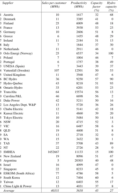
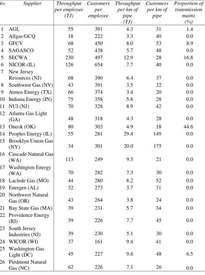
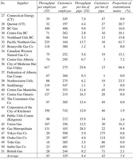
(9) i.e.. D0(x, y) = ιf/ι = exp (-u). (13). This measure represents the radial distance from the output vector to the frontier of the output set and therefore corresponds to the technical efficiency measure of Farrell (1957) and the output distance function defined in Shephard (1970). Continuing to follow Löthgren (1997), a log linear functional form is imposed on the ray function (12). ln ιi = αo +. M. ∑ j=1. βjlnx j + i. M + P −1. ∑. βjlnθ j-P + vi-ui , i = 1,…,N i. (14). j = M +1. The ray function (14) and firm specific technical efficiencies are estimated using the program FRONTIER 4.1 referred to above. 5. Data The data covers three industries: electricity, gas and telecommunications. The electricity industry data comprises 41 suppliers, each characterised by two outputs - electricity generated and customers served – and three inputs – hydro capacity, other capacity and full time employee equivalents. The gas industry data comprises 51 suppliers, each characterised by two outputs – gas sales and customers served – and three inputs - distribution mains, transmission pipeline and employees. The telecommunications industry comprises 31 suppliers, each characterised by five outputs – public pay phones, residential main lines, other main lines, international traffic, and cellular mobile subscribers – and two inputs – digital lines and employees. The data for each industry is summarised in tables 1 to 3. The international electricity data was obtained mainly from the Electricity Association (1996) and the annual report of China Light & Power Limited (1997). The Australian electricity supplier data was obtained from the Electricity Supply Association of Australia (1998). Most of the international data is centred around the year ending 1996. The Australian data is for the financial year ended 30 June 1997. The international data on gas suppliers was collected from a variety of sources including ANZ McCaughan (1992), American Gas Association (1993), Canadian Gas Association (1992), the Monopolies and Mergers Commission (1993) and the Japan Gas Association (1992). The Australian data was obtained from the Australian Gas Association (1994). The data on telecommunications was obtained in electronic form from the International Bank for Reconstruction and Development/World Bank (1992).. 6.

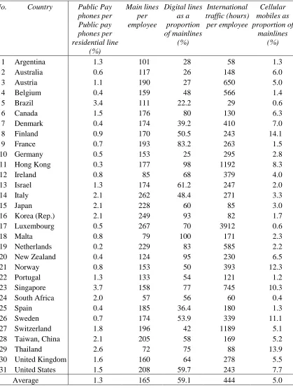
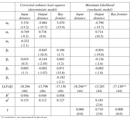
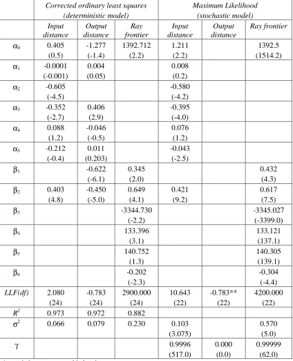
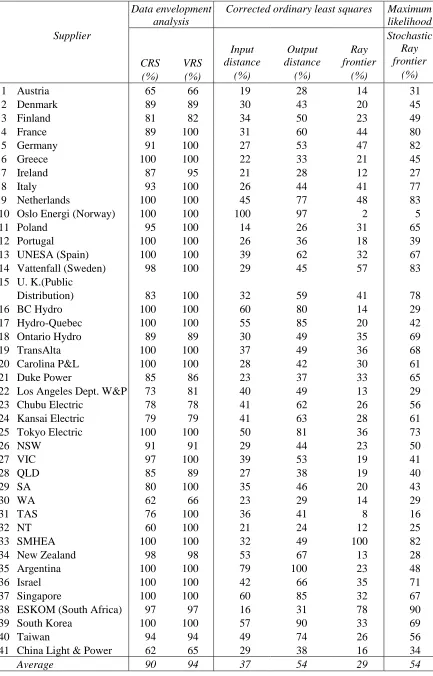
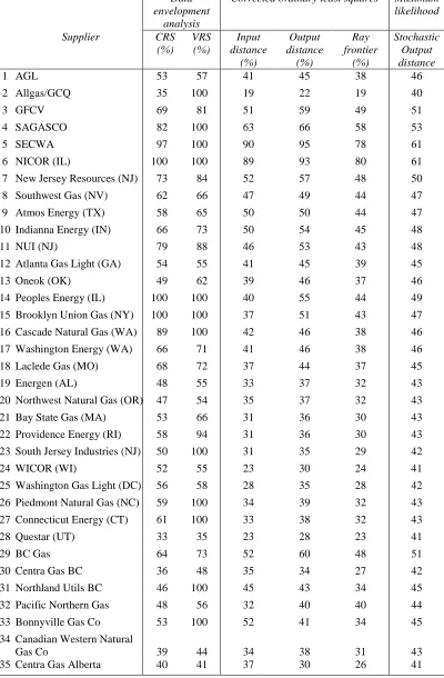
(10) 6. Results Three estimation techniques have been used in this study. These are nonparametric mathematical programming, parametric deterministic corrected ordinary least squares, and parametric stochastic maximum likelihood methods. Accordingly, eight different multiple-output technical efficiency models have been estimated for each of the electricity, gas and telecommunications industries. These models are:. 1.. Constant returns to scale (CRS) DEA,. 2.. Variable returns to scale (VRS) DEA,. 3.. Deterministic input distance function,. 4.. Deterministic output distance function,. 5.. Deterministic ray frontier function,. 6.. Stochastic input distance function,. 7.. Stochastic output distance function,. 8.. Stochastic ray frontier function.. DEA results The DEA results for the CRS and VRS models are provided in tables 7 to 9. On average the DEA estimates of technical efficiency are considerably higher than the estimates yielded by the stochastic frontier methodologies for all three industries. This runs counter to intuition which would suggest that the DEA and COLS estimates of technical efficiency fail to exclude the impact of stochastic factors and consequently should be somewhat lower, on average, than the corresponding estimates yielded by the stochastic distance and ray frontier models. Also, scale appears to play a bigger role in the gas industry than in the electricity and telecommunications industries according to the DEA results. COLS results The COLS estimates of the parameters of the deterministic Cobb-Douglas production frontier for the three industries are given in tables 4 to 6. The individual results are given for the input distance function, output distance 2 function and the ray frontier function. The R and many of the t-statistics are relatively high suggesting a reasonable fit of the data.. 7.

(11) The coefficient of employment (β 3) in the COLS output distance function for electricity is both significant and negative. The dependent variable in the equation is the negative of the natural logarithm of customer numbers. This implies that the elasticity of customer numbers with respect to employment is significant and positive. Likewise the coefficient of labour (β 1) in the COLS output distance function for gas is negative and statistically significant. The dependent variable in this case is the negative of the natural logarithm of gas sales. This therefore implies that the elasticity of gas sales with respect to employment is significant and positive. The coefficient of employment (β 1) in the COLS output distance function for telecommunications is negative and significant implying a positive elasticity of residential lines with respect to labour. The coefficient of employment (β 3) in the COLS ray frontier function for electricity is significant and negative. In this case the dependent variable in the ray frontier model is the natural logarithm of the norm defined over all outputs. This implies that the elasticity of the multiple output with respect to labour is negative. In the case of gas, the coefficient of labour (β 3) is significant and positive implying the expected positive elasticity of output with respect to labour. Likewise the coefficient of labour (β 1) in the COLS ray function for telecommunications is significant and positive. In the COLS distance equations for the gas industry, the coefficients of the transmission mains (β3) are statistically insignificant as is the coefficient of distribution mains (β2) in the input distance equation. Likewise the coefficient of transmission mains (β 2) in the COLS ray frontier equation for the gas industry is also statistically insignificant. Otherwise the input coefficients in the COLS equations are of expected sign and are statistically significant. The coefficients of pay phones (α1), international minutes (α4) and cellular mobile phones (α5) in the COLS distance equations for telecommunications are statistically insignificant. This suggests that the significant outputs for the telecommunications industry are residential mainlines (α2) and other main lines (α3). The average technical efficiency measured by the COLS output distance equation exceeds the technical efficiency measured by the COLS input distance equation for the electricity and gas industries. In theory output or input orientation should have no effect on resulting estimates of technical efficiency. In the case of the telecommunications industries the average technical efficiencies of the output and input distance functions are equal. The distance function estimates of technical efficiency on average exceed the ray frontier estimates. Again in theory estimates of the ray frontier and distance function models should be similar. However in the present case the. 8.

(12) ray frontier model has a single aggregated output whereas the distance function and the DEA estimates are based specifically on multiple outputs. ML results Stochastic input and output distance functions and stochastic ray frontier functions were estimated for each industry. However the input and output distance equations for the electricity industry, the output distance equation and the ray frontier equation for the gas industry, and the output distance equation for the telecommunications industry were found to have LLF values that were no different from the values obtained for the COLS equations. These results suggest that decomposition of the error into a systematic stochastic component (vi) and a one-sided technical efficiency component (ui) did not improve the results over those given by the deterministic COLS models. The corresponding estimates of the proportion of the error variance due to technical inefficiency (γ) were not statistically different from zero in the estimated equations. Accordingly the technical efficiency estimates yielded by these models have been ignored. The estimate of the proportion of the variance due to technical inefficiency (γ) for the stochastic ray frontier model of the electricity industry was estimated at 0.927. The corresponding estimate for the gas industry stochastic output distance function was 0.710. These results imply that while technical inefficiency accounts for most of the error, some stochastic error is present in the estimated models. The estimates of the proportion of the variance due to technical inefficiency (γ) for the stochastic input distance and ray frontier models of the telecommunications industry were estimated at unity implying that there was no stochastic error associated with the estimated equations. This is a rather extreme result. Coelli and Perelman (1996) also noted the unusual behavior of the ML estimation in yielding values of the parameter γ that were either zero or unity. They suggested that one possible cause for the ML estimator, selecting extreme values of γ, was the wide range in scales of operation of the railroad companies along with the second-order flexibility of the translog functional form. They contended that these factors could have resulted in the ML method adjusting the second order coefficients so that the translog function bent at extremities of the data range. As a result extreme observations would be quite close to the frontier thereby resulting in a distribution of residuals closely resembling a half-normal distribution. They supported this explanation with the observation that the same problems did not occur when the analysis was repeated with the simpler Cobb-Douglas form. However in the present study the Cobb-Douglas form has been used and we experience similar problems. Also, as outlined above, less extreme values of γ have been obtained for the stochastic ray frontier model of the electricity industry and the stochastic output distance function of the gas industry.. 9.

(13) Comparison of technical efficiency results Correlation matrices of the technical efficiency results for each industry are provided in tables 10–12. These matrices suggest that the technical efficiency estimates of the COLS input and output distance functions are highly correlated. Also there appears to be strong positive correlation between the technical efficiency estimates of the ML stochastic distance equations and the estimates yielded by the COLS distance equations. For instance, the COLS output distance technical efficiency estimates are perfectly correlated with the ML output distance technical efficiency estimates in the gas industry table 11. This suggests that given the problems with the ML estimator, either of the COLS distance functions could be preferred over the stochastic distance functions for estimating the technical efficiency of enterprises. The technical efficiency estimates yielded by the ray frontier models for the electricity industry are relatively uncorrelated with estimates yielded by DEA and the distance functions for the electricity industry in table 10. However the technical efficiency estimates yielded by the ray frontier models for gas and telecommunications are correlated with counterpart estimates yielded by the DEA and distance models in tables 11 and 12. This seems to suggest that the persistent finding of a negative and/or insignificant elasticity of output with respect to labour may be more a characteristic result for the electricity supply industry than other industries. A more focussed examination of technical efficiency in the electricity industry may be required. 7. Summary and conclusions This paper was motivated by the empirical observation that in many single output production function studies the elasticity of output with respect to labour was found to be insignificant and/or negative. It was suggested that many industries were characterised by multiple outputs and consequently that the application of single output models may yield misleading results particularly in relation to the sign and significance of the labour exponent of conventional production functions. Accordingly a number of multiple output efficiency measurement models have been applied to international data on the electricity, gas and telecommunications industries. The results suggest that the multiple output models are more likely to yield coefficients of labour with the expected positive sign. In an industry such as electricity, outputs include electricity generated as well as the number of customers served. Accordingly single output models focussing simply on electricity generated are likely to seriously underestimate the contribution of labour.. 10.

(14) In examining the above question a number of multiple output models were used. These included DEA models, deterministic distance function models, stochastic distance function models and deterministic and stochastic ray frontier models. The results suggest that the technical efficiency estimates yielded by the deterministic and stochastic models are highly correlated. Therefore given problems involved in estimating the stochastic models, the deterministic or corrected ordinary least squares models for estimating efficiency are to be preferred. Altogether the technical efficiency results, apart from those for the electricity industry, seem to be correlated. The DEA estimates of technical efficiency are, surprisingly, higher than comparable estimates yielded by the parametric methods. The main criticism of the DEA procedure has been that it does not exclude stochastic error and consequently that it would be likely to underestimate technical efficiency. Given the relatively high correlation between the technical efficiency estimates yielded by the deterministic and the frontier production models, the existence of stochastic error appears to have little impact on resulting estimates of technical efficiency. Also there appear to be major problems in estimating multiple output stochastic frontier models which make the parametric deterministic models or DEA preferred methodologies.. 11.

(15) REFERENCES Aigner, D.J., Lovell, C.A.K., & Schmidt, P. 1977, ‘Formulation and estimation of stochastic frontier production function models’, Journal of Econometrics 6, 21-37. ANZ McCaughan 1992, Gas and Fuel Corporation of Victoria: Future Ownership – Community and employee benefits, ANZ McCaughan: Melbourne, December. Australian Gas Association 1994, Gas Industry Statistics, Australian Gas Association: Canberra, June. Battese, G.E. & Coelli, T. J. 1988, ‘Prediction of firm-level technical efficiencies with a generalised frontier production function and panel data’, Journal of Econometrics, 38, 387-99. Canadian Gas Association 1992, Directory of Natural Gas Company Operations, Canadian Gas Association: Ontario, November. Charnes, A., Cooper, W.W. & Rhodes, E. 1978, ‘Measuring the efficiency of decision making units’, European Journal of Operational Research, 2, 429-44. China Light & Power Company, Limited 1997, Annual Report 1997, China Light and Power Ltd, Hong Kong. Coelli, T. J. 1996, ‘A guide to FRONTIER Version 4.1: A computer program for stochastic frontier production and cost function estimation’, Working Paper 96/07, Centre of Efficiency and Productivity Analysis, University of New England, Armidale, NSW, 2351. Coelli, T. 1998, ‘Productivity Growth in Australian Electricity Generation: Will the real TFP Measure please stand up?’, Centre for Efficiency and Productivity Analysis, University of New England, Armidale, June. Coelli, T & Perelman, S. 1996, ‘Efficiency measurement, multiple-output technologies and distance functions: with application to European Railways’, CREPP 96/05, Centre de Recherche en Economie Publique et en Economie de la Population, Université de Liège, May. Cowing , T.G. & Smith, V. K. 1980, ‘The Estimation of a Production Technology: A Survey of Econometric Analyses of Steam-Electric Generation’, Land Economics, 54, 156-186. Electricity Association 1998, International Electricity Prices, Issue 25, Electricity Supply Services Limited, 30 Millbank, London SWIP 4RD. Electricity Supply Association of Australia Limited (ESAA) 1994, International Performance Measurement for the Australian Electricity Supply Industry 1990-1991, Electricity Supply Association of Australia Limited, Level 11, 74 Castlereagh Street, Sydney NSW 2000. Electricity Supply Association of Australia Limited (ESAA) 1998, Electricity Australia 1998, Electricity Supply Association of Australia Limited, Level 11, 74 Castlereagh Street, Sydney NSW 2000. Fare, R., Grosskopf, S. & Lovell C.A.K. 1985, The Measurement of Efficiency of Production, Kuwer Academic Publishers, Boston. Farrell, M.J. 1957, ‘The measurement of productive efficiency’, Journal of the Royal Statistical Society, Series A, 120, 253-90.. 12.

(16) Greene, W. 1980, ‘Maximum Likelihood Estimation of Econometric Frontier Functions’, Journal of Econometrics, 13, 27-56. International Bank for Reconstruction and Development/World Bank 1992, ‘Socio-economic Time Series Access and Retrieval System’, Version 2.5, April (supplied on disk). Japan Gas Association 1992, Gas Facts in Japan, Japan Gas Association: Tokyo. Löthgren, M. 1997, ‘A Multiple Output Stochastic Ray Frontier Production Model’, Working Paper Series in Economics and Finance No. 158, Stockholm School of Economics, February. Löthgren, M. 1997, ‘Generalised stochastic frontier production models, Economics Letters 57, 255-259. Lovell, C.A.K, Richardson, S., Travers P. & Wood L.L. 1994, ‘Resources and Functionings: A New View of Inequality in Australia’, W. Eichhorn (ed.), Models and Measurement of Welfare and Inequality, Springer-Verlag: Berlin. Mardia, K.V., Kent, J.T. & Bibby, J.M. 1979, Multivariate Analysis, Academic Press: London. Monopolies and Mergers Commission 1993, Gas, Volume 1 of reports under the Fair Trading Act 1973 on the supply within Great Britain of gas through pipes to tariff and non-tariff customers, and supply within Great Britain of the conveyance and storage of gas by public gas suppliers, Monopoly and Mergers Commission: London, August. Quiggin, J. 1997, ‘Estimating the benefits of Hilmer and related reforms’, Australian Economic Review, 30, 256-72. Shephard, R.W. 1970, Theory of Cost and Production Functions, Princeton University Press: Princeton. Whiteman, J.L. 1999, ‘The Potential Benefits of Hilmer and Related Reforms: Electricity Supply’, Australian Economic Review, 32, 1, 17-30.. 13.

(17) Table 1: Summary of data on Electricity Suppliers No. Supplier. 1 2 3 4 5 6 7 8 9 10 11 12 13 14 15 16 17 18 19 20 21 22 23 24 25 26 27 28 29 30 31 32 33 34 35 36 37 38 39 40 41. Austria Denmark Finland France Germany Greece Ireland Italy Netherlands Oslo Energi (Norway) Poland Portugal UNESA (Spain) Vattenfall (Sweden) United Kingdom BC Hydro Hydro-Quebec Ontario Hydro TransAlta Carolina P&L Duke Power Los Angeles Dept. W&P Chubu Electric Kansai Electric Tokyo Electric NSW VIC QLD SA WA TAS NT SMHEA New Zealand Argentina Israel Singapore ESKOM (South Africa) South Korea Taiwan China Light & Power Average. Sales per customer (MWh). Productivity (MWh). 10 11 25 13 10 6 11 7 11 25 7 6 7 107 11 36 43 33 64 46 42 13 12 11 10 20 16 19 13 15 37 22 1652667 19 5 16 22 77 12 12 13 40331. 1617 3385 6009 3938 2606 1455 2184 1844 2911 6537 1004 1757 3443 12501 3568 9250 8218 6201 15574 6698 5211 5720 5141 4860 5484 4715 6487 4600 2718 3432 5708 2726 11133 8096 20303 4099 8233 4786 7404 6403 4031 5658. 14. Capacity factor (%) 32 41 48 53 51 48 51 37 46 34 46 38 39 50 47 57 51 53 56 56 50 36 42 39 50 52 58 51 32 30 43 28 15 51 40 47 45 58 60 55 37 45. Hydro capacity (%) 68 0 18 23 8 29 13 30 0 100 7 49 37 53 6 90 93 23 13 2 16 26 18 20 14 3 6 8 0 1 89 0 100 67 48 0 0 5 6 17 8 27.

(18) Table 2: Summary of data on Gas Suppliers No.. Supplier. 1 2 3 4 5 6 7. AGL Allgas/GCQ GFCV SAGASCO SECWA NICOR (IL) New Jersey Resources (NJ) Southwest Gas (NV) Atmos Energy (TX) Indiana Energy (IN) NUI (NJ) Atlanta Gas Light (GA) Oneok (OK) Peoples Energy (IL) Brooklyn Union Gas (NY) Cascade Natural Gas (WA) Washington Energy (WA) Laclede Gas (MO) Energen (AL) Northwest Natural Gas (OR) Bay State Gas (MA) Providence Energy (RI) South Jersey Industries (NJ) WICOR (WI) Washington Gas Light (DC) Piedmont Natural Gas (NC). 8 9 10 11 12 13 14 15 16 17 18 19 20 21 22 23 24 25 26. 31 40 53 48 28 40. Proportion of transmission mains (%) 1.4 0.0 8.9 0.0 16.8 0.0. 6.4 3.5 3.4 5.8 8.9. 37 32 20 28 42. 0.0 0.0 0.0 0.0 0.0. 318. 4.3. 28. 0.0. 80 55. 303 281. 4.9 29.4. 18 149. 44.6 0.0. 34. 301. 20.0. 175. 0.0. 113. 249. 9.5. 21. 0.0. 70. 282. 7.3. 30. 0.0. 44 32. 280 273. 8.2 3.7. 52 31. 0.0 0.0. 43. 264. 3.8. 24. 0.0. 39. 231. 5.7. 34. 0.0. 39. 226. 7.7. 45. 0.0. 39. 230. 5.1. 30. 0.0. 37. 161. 9.4. 41. 0.0. 45. 227. 9.6. 48. 6.5. 62. 226. 7.1. 26. 0.0. Throughput Customers per employee per (TJ) employee 55 18 68 52 230 126. 391 222 450 438 497 654. 68 43 66 75 70. 390 391 374 358 328. 48. 15. Throughput per km of pipe (TJ) 4.3 3.3 8.0 5.7 12.9 7.7. Customers per km of pipe.

(19) Table 2 (continued) No.. Supplier. 27 Connecticut Energy (CT) 28 Questar (UT) 29 BC Gas 30 Centra Gas BC 31 Northland Utils BC 32 Pacific Northern Gas 33 Bonnyville Gas Co 34 Canadian Western Natural Gas Co 35 Centra Gas Alberta 36 City of Medicine Hat Gas Utility 37 Federation of Alberta Gas Coops 38 Northwestern Utils 39 SaskEnergy 40 Centra Gas Manitoba 41 Centra Gas Ontario 42 The Consumers Gas Co 43 Corporation of the City of Kitchener 44 Public Utils Comm (Kingston) 45 Union Gas 46 Gaz Metropolitain 47 Tokyo Gas Co 48 Osaka Gas Co 49 Toho Gas 50 Saibu Gas Co 51 British Gas Average. Throughput Customers Throughput per employee per per km of (TJ) employee pipe (TJ). Customers per km of pipe. Proportion of transmission mains (%). 39. 245. 7.6. 47. 0.0. 32 100 71 86 225 118. 197 406 262 344 164 380. 4.4 9.0 2.8 3.3 13.7 1.2. 27 37 10 13 10 4. 20.7 16.0 10.1 15.8 61.7 8.0. 75. 252. 5.6. 19. 15.1. 74. 295. 0.7. 3. 7.2. 617. 275. 29.6. 13. 66.4. 67. 266. 0.3. 1. 0.0. 88 119 91 127. 275 547 353 215. 6.2 1.1 11.6 16.3. 19 5 45 28. 23.3 0.0 19.9 0.0. 97. 305. 15.4. 49. 0.0. 196. 742. 12.0. 46. 1.9. 98. 212. 15.9. 34. 107 131 20 25 16 23 28 85. 256 103 598 607 385 481 244 329. 12.5 28.5 5.9 4.6 3.5 5.2 8.2 8.4. 30 22 175 114 86 107 71 42. 3.9 16.3 9.8 0.8 0.0 0.0 0.0 2.1 7.4. 16.

(20) Table 3: Summary of data on Telecommunications suppliers No.. 1 2 3 4 5 6 7 8 9 10 11 12 13 14 15 16 17 18 19 20 21 22 23 24 25 26 27 28 29 30 31. Cellular Main lines Digital lines International Public Pay traffic (hours) mobiles as per as a phones per employee proportion per employee proportion of Public pay mainlines of mainlines phones per (%) (%) residential line (%) Argentina 1.3 101 28 58 1.3 Australia 0.6 117 26 148 6.0 Austria 1.1 190 27 650 5.0 Belgium 0.4 159 48 566 1.4 Brazil 3.4 111 22.2 29 0.6 Canada 1.5 176 80 130 6.3 Denmark 0.4 174 39.2 410 7.0 Finland 0.9 170 50.5 243 14.1 France 0.7 193 83.2 263 1.5 Germany 0.5 153 25 295 2.8 Hong Kong 0.3 177 98 1192 8.3 Ireland 0.8 85 68 379 4.0 Israel 1.3 174 61.2 247 2.0 Italy 2.1 262 48.4 271 3.3 Japan 2.1 228 60 85 3.0 Korea (Rep.) 2.1 249 93 82 1.7 Luxembourg 0.5 267 70 3912 0.6 Malta 0.8 79 100 171 2.3 Netherlands 0.2 229 83 585 2.2 New Zealand 0.4 124 95 230 6.5 Norway 0.8 153 50 393 12.3 Portugal 1.3 133 54 121 1.2 Singapore 3.7 158 77 745 10.3 South Africa 2.0 57 56 60 0.4 Spain 0.4 185 36.4 180 1.3 Sweden 0.7 174 53.9 339 11.1 Switzerland 1.8 196 42 1189 5.1 Taiwan, China 2.1 205 58 169 5.2 Thailand 2.6 72 75 88 13.9 United Kingdom 1.6 160 64 278 5.5 United States 1.5 208 59.7 243 7.7 Average 1.3 165 59.1 444 5.0 Country. 17.

(21) Table 4: Estimated parameters for alternative models: Electricity*. α0 α1 α2 β1 β2 β3 β4 LLF(df) R2 σ2. Corrected ordinary least squares (deterministic model) Input Output Ray distance distance frontier -2.936 0.926 -7406.110 (-2.8) (-2.7) (0.9) -0.527 0.596 (-5.1) (8.0) -0.487 (-6.7) 0.017 -0.023 0.835 (1.7) (-2.6) (4.7) 0.218 -0.198 0.031 (5.4) (-5.4) (1.9) -0.636 -0.273 (-10.0) (-2.9) 16429.238 (2.8) -21.565 -18.119 -40.544 (36) (36) (36) 0.914 0.979 0.720 0.191 0.161 0.482. γ. Maximum Likelihood (stochastic model) Input Output Ray frontier distance distance -7405.297 (-14680.7). -21.565** (34). 0.000 (0.0). * t-statistics are presented in brackets. **The likelihood value is less than that obtained from the OLS model.. 18. -18.119** (34). 0.812 (8.7) 0.034 (3.0) -0.287 (-5.4) 16429.386 (17190.1) -38.023 (34). 0.000 (0.0). 1.020 (3.1) 0.927 (10.7).

(22) Table 5: Estimated parameters for alternative models: Gas*. α0 α1 α2 β1 β2 β3 β4 LLF(df) R2 σ2. Corrected ordinary least squares (deterministic model) Input Output Ray distance distance frontier 5.376 -5.084 5.470 (13.2) (-15.7) (15.9) -0.769 0.718 (-9.3) (9.9) -0.222 (-2.1) -0.845 0.106 (-16.5) (1.7) 0.019 -0.144 0.003 (0.3) (-2.45) (1.2) 0.003 -0.002 0.871 (1.1) (-1.07) (15.8) -0.182 (-2.1) -18.296 -13.798 -17.130 (46) (46) (46) 0.956 0.949 0.958 0.133 0.112 0.127. γ. Maximum Likelihood (stochastic model) Input Output Ray frontier distance distance -4.790 (-15.7) 0.714 (10.3). -0.854 (-19.0) -0.136 (-2.6) -0.002 (-1.0). -18.296** (44). -13.283 (44). -17.130** (44). 0.000 (0.0). 0.183 (2.6) 0.710 (3.0). 0.000 (0.0). * t-statistics are presented in brackets. **The likelihood value is less than that obtained from the OLS model.. 19.

(23) Table 6: Estimated parameters for alternative models: Telecommunications*. α0 α1 α2 α3 α4 α5 β1 β2 β3 β4 β5 β6 LLF(df) R2 σ2. Corrected ordinary least squares (deterministic model) Input Output Ray distance distance frontier 0.405 -1.277 1392.712 (0.5) (-1.4) (2.2) -0.0001 0.004 (-0.001) (0.05) -0.605 (-4.5) -0.352 0.406 (-2.7) (2.9) 0.088 -0.046 (1.2) (-0.5) -0.212 0.011 (-0.4) (0.203) -0.622 0.345 (-6.1) (2.0) 0.403 -0.450 0.649 (4.8) (-5.0) (4.1) -3344.730 (-2.2) 133.396 (3.1) 140.752 (1.3) -0.202 (-2.3) 2.080 -0.783 2900.000 (24) (24) (24) 0.973 0.972 0.882 0.066 0.079 0.230. γ. Maximum Likelihood (stochastic model) Input Output Ray frontier distance distance 1.211 1392.5 (2.2) (1514.2) 0.008 (0.2) -0.580 (-4.2) -0.395 (-4.0) 0.076 (1.2) -0.043 (-2.5) 0.432 (4.3) 0.421 0.617 (9.2) (7.5) -3345.027 (-3399.0) 133.121 (137.1) 140.305 (139.1) -0.304 (-4.4) 10.643 -0.783** 4200.000 (22) (22) (22) 0.103 (3.075) 0.9996 (517.0). * t-statistics are presented in brackets. **The likelihood value is less than that obtained from the OLS model.. 20. 0.000 (0.0). 0.570 (5.0) 0.99999 (62.0).

(24) Table 7: Technical efficiency for alternative models: Electricity Data envelopment analysis. Corrected ordinary least squares. Supplier. 1 2 3 4 5 6 7 8 9 10 11 12 13 14 15 16 17 18 19 20 21 22 23 24 25 26 27 28 29 30 31 32 33 34 35 36 37 38 39 40 41. Austria Denmark Finland France Germany Greece Ireland Italy Netherlands Oslo Energi (Norway) Poland Portugal UNESA (Spain) Vattenfall (Sweden) U. K.(Public Distribution) BC Hydro Hydro-Quebec Ontario Hydro TransAlta Carolina P&L Duke Power Los Angeles Dept. W&P Chubu Electric Kansai Electric Tokyo Electric NSW VIC QLD SA WA TAS NT SMHEA New Zealand Argentina Israel Singapore ESKOM (South Africa) South Korea Taiwan China Light & Power Average. CRS (%) 65 89 81 89 91 100 87 93 100 100 95 100 100 98. VRS (%) 66 89 82 100 100 100 95 100 100 100 100 100 100 100. Input distance (%) 19 30 34 31 27 22 21 26 45 100 14 26 39 29. Output distance (%) 28 43 50 60 53 33 28 44 77 97 26 36 62 45. 83 100 100 89 100 100 85 73 78 79 100 91 97 85 80 62 76 60 100 98 100 100 100 97 100 94 62 90. 100 100 100 89 100 100 86 81 78 79 100 91 100 89 100 66 100 100 100 98 100 100 100 97 100 94 65 94. 32 60 55 30 37 28 23 40 41 41 50 29 39 27 35 23 36 21 32 53 79 42 60 16 57 49 29 37. 59 80 85 49 49 42 37 49 62 63 81 44 53 38 46 29 41 24 49 67 100 66 85 31 90 74 38 54. 21. Maximum likelihood Stochastic Ray Ray frontier frontier (%) (%) 14 31 20 45 23 49 44 80 47 82 21 45 12 27 41 77 48 83 2 5 31 65 18 39 32 67 57 83 41 14 20 35 36 30 33 13 26 28 36 23 19 19 20 14 8 12 100 13 23 35 32 78 33 26 16 29. 78 29 42 69 68 61 65 29 56 61 73 50 41 40 43 29 16 25 82 28 48 71 67 90 69 56 34 54.

(25) Table 8: Technical efficiency for alternative models: Gas. Supplier. Data envelopment analysis CRS VRS (%) (%). Corrected ordinary least squares. Maximum likelihood. Output distance (%) 45. Ray frontier (%) 38. Stochastic Output distance 46. 1 AGL. 53. 57. Input distance (%) 41. 2 Allgas/GCQ. 35. 100. 19. 22. 19. 40. 3 GFCV. 69. 81. 51. 59. 49. 51. 4 SAGASCO. 82. 100. 63. 66. 58. 53. 5 SECWA. 97. 100. 90. 95. 78. 61. 6 NICOR (IL). 100. 100. 89. 93. 80. 61. 7 New Jersey Resources (NJ). 73. 84. 52. 57. 48. 50. 8 Southwest Gas (NV). 62. 66. 47. 49. 44. 47. 9 Atmos Energy (TX). 58. 65. 50. 50. 44. 47. 10 Indianna Energy (IN). 66. 73. 50. 54. 45. 48. 11 NUI (NJ). 79. 88. 46. 53. 43. 48. 12 Atlanta Gas Light (GA). 54. 55. 41. 45. 39. 45. 13 Oneok (OK). 49. 62. 39. 46. 37. 46. 14 Peoples Energy (IL). 100. 100. 40. 55. 44. 49. 15 Brooklyn Union Gas (NY). 100. 100. 37. 51. 43. 47. 16 Cascade Natural Gas (WA). 89. 100. 42. 46. 38. 46. 17 Washington Energy (WA). 66. 71. 41. 46. 38. 46. 18 Laclede Gas (MO). 68. 72. 37. 44. 37. 45. 19 Energen (AL). 48. 55. 33. 37. 32. 43. 20 Northwest Natural Gas (OR). 47. 54. 35. 37. 32. 43. 21 Bay State Gas (MA). 53. 66. 31. 36. 30. 43. 22 Providence Energy (RI). 58. 94. 31. 36. 30. 43. 23 South Jersey Industries (NJ). 50. 100. 31. 35. 29. 42. 24 WICOR (WI). 52. 55. 23. 30. 24. 41. 25 Washington Gas Light (DC). 56. 58. 28. 35. 28. 42. 26 Piedmont Natural Gas (NC). 59. 100. 34. 39. 32. 43. 27 Connecticut Energy (CT). 61. 100. 33. 38. 32. 43. 28 Questar (UT). 33. 35. 23. 28. 23. 41. 29 BC Gas. 64. 73. 52. 60. 48. 51. 30 Centra Gas BC. 36. 48. 35. 34. 27. 42. 31 Northland Utils BC. 46. 100. 45. 43. 34. 45. 32 Pacific Northern Gas. 48. 56. 32. 40. 40. 44. 33 Bonnyville Gas Co. 53. 100. 52. 41. 34. 45. 34 Canadian Western Natural Gas Co 35 Centra Gas Alberta. 39 40. 44 41. 34 37. 38 30. 31 26. 43 41. 22.

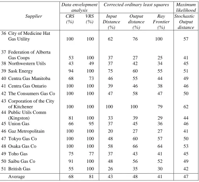
(26) Table 8 (Continued). Supplier. Data envelopment analysis CRS VRS (%) (%). Corrected ordinary least squares Input Distance (%). Output distance (%). Maximum likelihood Ray Stochastic Frontier Output (%) distance. 36 City of Medicine Hat Gas Utility. 100. 100. 62. 76. 100. 57. 37 Federation of Alberta Gas Coops 38 Northwestern Utils. 53 43. 100 49. 37 37. 27 42. 25 34. 41 45. 39 Sask Energy. 94. 100. 75. 60. 55. 51. 40 Centra Gas Manitoba. 68. 73. 46. 55. 44. 49. 41 Centra Gas Ontario. 100. 100. 39. 46. 38. 46. 42 The Consumers Gas Co. 100. 100. 47. 58. 47. 50. 100. 100. 100. 100. 79. 62. 81 66. 100 95. 33 37. 39 45. 29 36. 44 46. 46 Gaz Metropolitain. 100. 100. 20. 27. 27. 41. 47 Tokyo Gas Co. 100. 100. 48. 60. 57. 50. 48 Osaka Gas Co. 43 Corporation of the City of Kitchener 44 Public Utils Comm (Kingston) 45 Union Gas. 100. 100. 58. 66. 64. 53. 49 Toho Gas. 75. 77. 37. 43. 41. 45. 50 Saibu Gas Co. 91. 100. 48. 56. 52. 49. 51 British Gas. 55. 100. 26. 35. 30. 42. Average. 68. 81. 43. 48. 41. 47. 23.

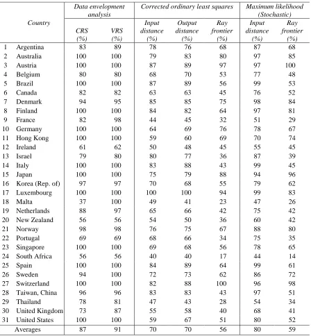
(27) Table 9: Technical efficiency for alternative models: Telecommunications Data envelopment analysis Country. 1 2 3 4 5 6 7 8 9 10 11 12 13 14 15 16 17 18 19 20 21 22 23 24 25 26 27 28 29 30 31. Argentina Australia Austria Belgium Brazil Canada Denmark Finland France Germany Hong Kong Ireland Israel Italy Japan Korea (Rep. of) Luxembourg Malta Netherlands New Zealand Norway Portugal Singapore South Africa Spain Sweden Switzerland Taiwan, China Thailand United Kingdom United States Averages. CRS (%) 83 100 100 80 100 82 94 100 82 100 100 61 79 100 100 97 100 37 88 56 98 69 100 56 100 94 100 96 78 73 100 87. VRS (%) 89 100 100 80 100 82 95 100 98 100 100 62 80 100 100 97 100 100 97 56 98 69 100 56 100 100 100 96 81 87 100 91. Corrected ordinary least squares Input distance (%) 78 79 87 68 87 63 85 84 44 64 59 50 80 83 75 70 100 49 65 54 76 68 69 40 84 72 82 83 47 55 59 70. 24. Output distance (%) 76 83 89 70 89 63 85 82 45 69 60 48 77 88 79 68 100 41 66 50 75 66 68 40 89 73 88 83 43 58 67 70. Ray frontier (%) 68 80 97 53 56 45 75 64 32 76 69 45 36 43 88 55 94 23 42 36 67 34 56 17 64 62 100 43 28 40 51 56. Maximum likelihood (Stochastic) Input Ray distance frontier (%) (%) 87 68 97 85 97 100 77 48 99 53 76 52 98 84 97 81 51 29 78 67 70 74 55 45 87 39 99 45 94 96 79 62 99 83 47 26 75 42 60 42 88 80 75 35 78 65 44 14 99 61 86 72 96 98 97 51 54 34 68 41 80 52 80 59.

(28) Table 10: Correlation table of alternative technical efficiency measures: Electricity. DEA CRS DEA VRS COLS Input distance COLS Output distance COLS Ray frontier ML Ray frontier. DEA CRS. DEA VRS. COLS Input distance. COLS Output distance. COLS ML Ray Ray frontier frontier. 1.00 0.75. 1.00. 0.40. 0.26. 1.00. 0.51. 0.33. 0.92. 1.00. 0.37. 0.28. -0.24. -0.02. 1.00. 0.41. 0.30. -0.24. 0.08. 0.85. 1.00. Table 11: Correlation table of alternative technical efficiency measures: Gas. DEA CRS DEA VRS COLS Input distance COLS Output distance COLS Ray frontier ML Output distance. DEA CRS. DEA VRS. COLS Input distance. 1.00 0.68. 1.00. 0.57. 0.34. 1.00. 0.69. 0.38. 0.94. 1.00. 0.69. 0.38. 0.87. 0.94. 1.00. 0.69. 0.39. 0.94. 1.00. 0.95. 25. COLS Output distance. COLS ML Ray Output frontier distance. 1.00.

(29) Table 12: Correlation table of alternative technical efficiency measures: Telecommunications. DEA CRS DEA VRS COLS Input distance COLS Output distance COLS Ray frontier ML Input distance ML Ray frontier. DEA CRS. DEA VRS. COLS COLS Input Output distance distance. 1.00 0.73. 1.00. 0.69. 0.51. 1.00. 0.77. 0.56. 0.98. 1.00. 0.71. 0.56. 0.69. 0.74. 1.00. 0.79. 0.58. 0.96. 0.98. 0.72. 1.00. 0.72. 0.57. 0.69. 0.71. 0.96. 0.73. 26. COLS Ray frontier. ML Input distance. ML Ray frontier. 1.00.

(30)

No results found