Cryptographic pairings
Kristin Lauter and Michael Naehrig
Microsoft Research, Redmond, USA
Abstract
Contents
9 Cryptographic Pairings page1
9.1 Preliminaries 3
9.1.1 Elliptic curves 3
9.1.2 Pairings 4
9.1.3 Pairing-friendly elliptic curves 7
9.2 Finite field arithmetic for pairings 8
9.2.1 Montgomery multiplication 9
9.2.2 Multiplication in extension fields 10
9.2.3 Finite field inversions 10
9.2.4 Simultaneous inversions 13
9.3 Affine coordinates for pairing computation 14 9.3.1 Costs for doubling and addition steps 14
9.3.2 Working over extension fields 18
9.3.3 Simultaneous inversions in pairing computation 19
9.4 The double-add operation and parabolas 22
9.4.1 Description of the algorithm 22
9.4.2 Application to scalar multiplication 23
9.4.3 Application to pairings 24
9.5 Squared pairings 26
9.5.1 The squared Weil pairing 26
9.5.2 The squared Tate pairing 27
Bibliography 29
9
Cryptographic Pairings
Kristin Lauter and Michael Naehrig
During more than 15 years as a Principal Researcher at Microsoft Research, Peter L. Montgomery contributed substantially to building the public key crypto-graphy libraries for Microsoft. The field of Elliptic Curve Cryptocrypto-graphy (ECC) was scarcely 15 years old, and pairing-based cryptography had been recently introduced, when Peter started working on implementing and optimizing crypt-ographic pairings on elliptic and hyperelliptic curves.
Bypairingson elliptic curves in the cryptographic setting, we are referring to bilinear maps from the group of points on an elliptic curve to the multi-plicative group of a finite field, most notably theWeilpairing. Cryptographic pairings became a hot topic after the introduction of solutions for various interesting cryptographic primitives, including identity-based non-interactive key agreement [55], one-round tripartite Diffie–Hellman key exchange [44, 45], identity-based encryption [16] and short signatures [18, 19]. A flood of other cryptographic applications and constructions followed, such as attribute-based encryption [54], functional encryption [20], and homomorphic encryp-tion [17], to name a few. Pairings originally played a key role in the earlier Menezes-Okamoto-Vanstone [49] and Frey-Rück [31] attacks on supersingu-lar elliptic curves, which had instead negative implications for cryptographic primitives using such curves. All cryptographic applications of pairings rely on the ability to find suitable elliptic curve parameters and the existence of ef-ficient algorithms to compute in the groups involved in the pairing operation and for the pairing computation itself.
This chapter is based on the three papers, [27], [28] and [48] on pairing computation, which Peter coauthored with one or both of the authors. The text contains excerpts from those works, lightly edited with adjustments made to unify notation and embed into the context of this chapter.
giving formulas for the often pesky case of characteristic two. The code he wrote was usually intended to be most general in the sense that it should allow to be compiled and run efficiently and securely on a wide variety of possible processors. And he produced side-channel resistant implementations without even mentioning the existence of such attacks. In his implementations of el-liptic curve cryptography, Peter often used Montgomery multiplication for the base field arithmetic, assuming operations would be carried out modulo general primes, and would not rely on generalized Mersenne primes or other primes with special reduction, for example. Peter used to significantly speed up mod-ular inversion in his implementations, which led to a low ratio for the cost of inversion to multiplication.
Several other signature ideas from Peter’s work played a role in optimiz-ing algorithms for pairoptimiz-ing computation. In addition to fast modular inversion, Peter also introduced the widely used simultaneous inversion trick [52, Sec-tion 10.3.1.] (see Chapter 1), which can be applied to pairing computaSec-tion as explained in Section 9.3 on page 14. In general, achieving a low ratio of inver-sion to multiplication cost through this collection of tricks in various settings favors affine coordinates, which is relevant, for example, in application sce-narios such as the computation of multiple pairings, products of pairings, and parallelized pairings, as well as for pairings at very high security levels. These applications are all explained in Section 9.3.
In another direction, the Montgomery ladder [52] (see Chapter 4) used in the ECM factoring method (see Chapter 8) does not need they-coordinate of the elliptic curve points and allows the efficient computation of scalar multi-plication using x-coordinates only. In Section 9.4 on page 22, we present the double-and-add trick from [27], which saves a multiplication in combined op-erations by not computing the intermediate y-coordinate. Also, the squared Weil and Tate pairings, presented in Section 9.5 on page 26, achieve cancel-lation of vertical line function contributions because they only depend on the x-coordinates, which are equal for a point and its negative.
9.1 Preliminaries
We start by introducing notation and describing the basic concepts needed to talk about cryptographic pairings and their computation, such as elliptic curves, their group law, pairings and pairing-friendly elliptic curves. To ease the exposition, the material is not presented in the most general setting, but rather focused on special cases that are most common and representative of the general ideas. For more details, we point the reader to [60, 13, 25, 26, 32].
9.1.1 Elliptic curves
Letp>3 be a prime andFqbe a finite field of characteristicp. Throughout the
whole chapter, we considerEto be an elliptic curve defined overFq, given by a
short Weierstrass equationE:y2=x3+ax+b, wherea,b∈
Fqand 4a3+27b2,
0. The point at infinity onEis denoted byO. The curveE can be viewed as the set of affine solutions (x,y) of the curve equation with coordinates in an algebraic closure ofFqtogether with the special pointO. The set ofFq-rational
points onEis given byE(Fq) ={(x,y) ∈ Fq×Fq | y2 = x3+ax+b} ∪ {O},
and the number of such points isn =#E(Fq)=q+1−t, wheretis bounded
by|t| ≤2√q.
The group law
There exists an abelian group law+onE, which is given as follows. The point
Ois the neutral element, i.e.,P1+O=P1for any pointP1∈E. IfP1,O, write
P1=(x1,y1). Then, the inverse element ofP1is the point−P1=(x1,−y1), i.e.,
(x1,y1)+(x1,−y1) = O. Given another pointP2 = (x2,y2) ∈ E \ {O,−P1},
define
λ=
(y2−y1)/(x2−x1) ifP1,P2,
(3x21+a)/(2y1) ifP1=P2.
(9.1)
ThenP3=(x3,y3)=P1+P2is given byx3=λ2−x1−x2andy3=λ(x1−x3)−y1.
Computing the sum of two affineFq-rational points requires a division in the
fieldFq. This operation is usually significantly more costly than all the other
Embedding degree and torsion points
Let r be a prime with r | n, and letk be the embedding degree ofE with respect tor, i. e.kis the smallest positive integer withr| qk−1. This means
that the multiplicative group F∗
qk contains as a subgroup the groupµr of r
-th roots of unity. The embedding degree kis an important parameter, since it determines the field extensions over which the groups that are involved in pairing computation are defined.
Form ∈Z, let [m] : E → Ebe the multiplication-by-mmap, which maps a pointP ∈ E to the sum ofmcopies of P. The kernel of [m] is the set of m-torsion points onE; it is denoted byE[m] and we writeE(Fq`)[m] for the set
ofFq`-rationalm-torsion points (` >0). From now on it is assumed thatk>1,
in which caseE[r]⊆E(Fqk), i.e., allr-torsion points are defined overFqk.
9.1.2 Pairings
In order to describe the pairing functions relevant to cryptography, we need to introduce divisors onE. A divisorDonEis a formal sum of points with integer coefficients, i.e., D= P
P∈EnP(P) with only finitely many of thenP different
from zero; this finite set of non-zeronP-values is the support of the divisorD.
A divisor is called a principal divisor, if it is the divisor of a function f onE. In that case the coefficientnPreflects the multiplicity ofPas a zero (ifnP>0)
or pole (nP <0) of f. Two divisors are equivalent if they differ by a principal
divisor. ForP1 ∈ E, let DP1 be a divisor that is equivalent to (P1)−(O). Let
fr,P1be a function onEwith divisorr(P1)−r(O). Evaluating a function f at a
divisorPn
P(P) means to evaluateQf(P)np.
The Weil pairing
The first applications of pairings in cryptography used the Weil pairing er=E[r]×E[r]→µr⊆F∗qk, (P,Q)7→ fr,P(DQ)/fr,Q(DP).
For the computation of fr,Q(DP), we can take DQ = (Q)−(O) and need to
choose a suitable pointRsuch thatDP = (P+R)−(R) has support disjoint
from{O,Q}(and similarly for fr,P(DQ)).
The Tate pairing
Most pairings that are suitable for use in practical cryptographic applications are derived from the reduced Tate pairing
tr=E(Fq)[r]×E(Fqk)[r]→µr⊆F∗
qk, (P,Q)7→ fr,P(DQ)(q
k−1)/r
.
In the casek>1, to which we restrict in this chapter, one can omit the auxiliary point in the divisorDQand compute fr,P(Q)(q
k−1)/r
Miller’s algorithm
To evaluate the functions occurring in the Weil and the Tate pairing, one fol-lows an iterative approach based on Miller’s formulas [50]. For an integer m ∈ Z and a point P ∈ E(Fqk)[r] define the function fm,P to be a function with divisorm(P)−([m]P)−(m−1)(O). Note that this notation coincides with the one used above form=rbecause then [r]P=O. The value of the function fr,Pat the pointQcan be computed in a square-and-multiply-like fashion via
function values fm,P(Q) form<rwith the help of certain line functions. Let
P1,P2,Q ∈ E such thatP1 , O, P2 < {O,−P1}, andE , O. Then the line
throughP1=(x1,y1) andP2=(x2,y2), evaluated atQ=(xQ,yQ) is given by
lP1,P2(Q)=(yQ−y1)−λ(xQ−x1),
whereλis the value of the slope computed during the computation ofP1+P2as
in Equation (9.1) on page 3. In the case thatP2=−P1, we have the vertical line
function valuevP1(Q)=lP1,−P1(Q)=xQ−x1. Define the quotientgP1,P2(Q)=
lP1,P2(Q)/vP1+P2(Q). Then, form1,m2∈Z, Miller’s formulas hold as follows:
fm1+m2,P(Q)= fm1(Q)fm2(Q)g[m1]P,[m2]P(Q),
fm1m2,P(Q)= f
m2
m1(Q)fm2,[m1]P(Q)= f
m1
m2(Q)fm1,[m2]P(Q).
Specializations of these formulas yield fm+1,P(Q) = fm,P(Q)g[m]P,P(Q), and
f2m,P(Q) = fm2,P(Q)g[m]P,[m]P(Q), which lead to Miller’s algorithm to compute
fr,P(Q) as shown in Algorithm 1 on page 5. Note that as written here, in the last
iteration of the algorithm, sincer0 =1, the point addition in line 5 computes
the point at infinityOin an exceptional case. The value of the functiongR,Pin
this step is defined asgR,P(Q)=vP(Q).
Algorithm 1Miller’s algorithm
Input: P,Q∈E[r],r=(r`−1,r`−2, . . . ,r0)2,r`−1=1 Output: fr,P(Q) representing a class inF∗qk/(F
∗
qk)
r
1: R←P, f ←1
2: forifrom`−1 downto 0do
3: f ← f2·g
R,R(Q), R←[2]R
4: if(mi=1)then
5: f ← f ·gR,P(Q), R←R+P
6: end if
7: end for
8: return f
groups, which multiply curve points by varying scalars that are often secret val-ues in the respective cryptographic protocols, Miller’s algorithm works along-side a scalar multiplication with a fixed scalar, namelyr. In other words, the exponentiation carried out in Miller’s algorithm is always to the same public number. Significant savings can be obtained by choosing this system parameter with a low Hamming weight (or low weight in a signed binary representation) in order to have as few as possible of the addition steps in line 5 of Algorithm 1. The final exponentiation to the power (qk−1)/r in the Tate pairing after
the Miller loop represents a large part of the computation. It maps classes inF∗
qk/(F ∗
qk)
r to unique representatives inµ
r and is an exponentiation with a
known fixed, special exponent. Parts of it are carried out in special subgroups of the multiplicative group F∗
qk. This leads to various improvements over a general exponentiation with an exponent of that size, leading to a significant speedup (see, for example [59, 35, 39]).
The ate pairing
Often the most efficient choices for implementation are variants of the ate pair-ing [41], which is a certain power of the reduced Tate pairpair-ing and is defined on special subgroups ofE[r].
Letφqbe theq-power Frobenius endomorphism onE, i.e.,φq(x,y)=(xq,yq).
Define two groups of prime orderrbyG1 =E[r]∩ker(φq−[1]) =E(Fq)[r]
andG2 =E[r]∩ker(φq−[q])⊆E(Fqk)[r]. The groupG1contains only points defined over the base fieldFq, while the points inG2 are minimally defined
overFqk. Theate pairingis the map
aT :G2×G1→µr, (Q,P)7→ fT,Q(P)(q
k−1)/r
, (9.2)
whereT = t−1. The groupG2 has a nice representation by an isomorphic
group of points on a twistE0of E, which is a curve that is isomorphic to E. Here, we are interested in those twists which are defined over a subfield ofFqk such that the twisting isomorphism is defined overFqk. Such a twistE0ofEis given by an equationE0 : y2 = x3+(a/α4)x+(b/α6) for someα∈
Fqk with isomorphismψ:E0→ E, (x,y)7→(α2x, α3y). Ifψis minimally defined over Fqk andE0is minimally defined overFqk/d for ad | k, then we say thatE0is a twist of degreed. Ifa =0, letd0 =4; ifb =0, letd0 =6, and letd0 =2
otherwise. Ford=gcd(k,d0) there exists exactly one twistE0ofEof degreed
for whichr|#E0(Fqk/d) (see [41]). DefineG02=E
0(
Fqk/d)[r]. Then the mapψis
a group isomorphismG02→G2and we can represent all elements inG2by the
corresponding preimages inG0
2. Likewise, all arithmetic that needs to be done
defined over a smaller field than those inG2. UsingG02, we may now view the
ate pairing as a mapG02×G1→µr, (Q0,P)7→ fT,ψ(Q0)(P)(q
k−1)/r .
Algorithm 2 shows Miller’s algorithm in the just described setting for an ate-like pairing to compute fm,ψ(Q0)(P) for some integerm >0. In this algorithm
and throughout the rest of this chapter, we assume thatkis even and therefore the denominator elimination technique applies (see [8, 9]), which means that the denominators in the above defined fractiongQ0
1,Q
0
2(P) of line functions can
be omitted without changing the pairing value. This is why Algorithm 2 only uses the line functionslQ0
1,Q
0
2(P).
Algorithm 2Miller’s algorithm for evenkand ate-like pairings
Input: Q0∈G0
2,P∈G1,m=(ml−1,ml−2, . . . ,m0)2,ml−1=1 Output: fm,ψ(Q0)(P) representing a class inF∗
qk/(F ∗
qk)
r
1: R0←Q0, f ←1
2: forifrom`−1 downto 0do
3: f ← f2·lψ(R0),ψ(R0)(P), R0←[2]R0
4: if(mi=1)then
5: f ← f ·lψ(R0),ψ(Q0)(P), R0←R0+Q0
6: end if
7: end for 8: return f
Miller’s algorithm builds up the function value fm,ψ(Q0)(P) along a scalar
multiplication computing [m]Q0(which is the value ofR0after the Miller loop). Step 3 is called adoubling step, it consists of squaring the intermediate value f ∈ Fqk, multiplying it with the function value given by the tangent to E at R=ψ(R0), and doubling the pointR0. Similarly, anaddition stepis computed in step 5 of Algorithm 2.
The most efficient variants of the ate pairing are so-called optimal ate pair-ings [61]. They are optimal in the sense that they minimize the size ofmand with that the number of iterations in Miller’s algorithm to log(r)/ϕ(k), where
ϕis the Euler totient function and log is the logarithm to base 2. For such min-imal values ofm, the function fm,ψ(Q0) alone usually does not give a bilinear
map. To get a pairing, these functions need to be adjusted by multiplying with a small number of line function values (see [61] for details).
9.1.3 Pairing-friendly elliptic curves
pairing-friendly, i.e., the embedding degree kneeds to be small, whiler should be larger than √q. A survey of methods to construct such curves can be found in [29]. For security reasons, the parameters need to have certain minimal sizes which imply suitable values for the embedding degreekfor specific security levels.
The requirement for an elliptic curve to have small embedding degree is a strong condition that restricts the set of possible curves to a small subset of elliptic curves. Because of the possibility of a transfer attack on the dis-crete logarithm problem like the Menezes-Okamoto-Vanstone [49] or the Frey-Rück [31, 30] attacks, such curves are excluded from being used in elliptic curve-based protocols that do not require a pairing function. In general, an ar-bitrary elliptic curve over a finite field with a large prime divisor of the group order will have a large embedding degree. This means that pairing-friendly curves are special and rare and finding a curve that satisfies the required prop-erties can be a challenge.
The most popular choices for pairing-friendly curves come from polynomial families of curves. In these families, the base field prime and the prime group order are parameterized by rational polynomials that ensure all conditions are satisfied. Concrete parameters are obtained by searching for an integer param-eter such that the above polynomials evaluate to prime integers at the parame-ter. A corresponding elliptic curve can then be constructed using the complex multiplication method, or a simpler algorithm that tests for the correct group order in certain special cases.
As explained in subsection 9.1.2 on page 6, it is often advantageous to choose curves with twists of degree 4 or 6, so-called high-degree twists, since this results in higher efficiency due to the more compact representation of the groupG2. To achieve security levels of 128 bits or higher, embedding degrees
of 12 and larger are advantageous. Because the degree of the twist E0 is at most 6, this means that when computing ate-like pairings at such security lev-els, all field arithmetic in the doubling and addition steps in Miller’s algorithm takes place over a proper extension field ofFq.
9.2 Finite field arithmetic for pairings
This section takes a closer look at the field arithmetic needed for pairing al-gorithms. As above, letFqbe a finite field of characteristicp>3, and letFqm be an extension of degreemofFqform|k. Note that mostly, pairing-friendly
some of the field extensionsFqm. A crucial building block with major influence on the overall efficiency of pairing-based protocols is multiplication modulo the primep. An obvious influence of Peter’s work is the use of Montgomery arithmetic for modular operations.
Another aspect that has been inspired by Peter’s way of thinking is the treat-ment of inversions. As indicated above, usually the cost for a field inversion is larger than that for a field multiplication, which in turn is larger than that for an addition and a subtraction. What the exact ratios between these are, depends on the setting, i.e., the shape of the base field prime, the extension degree, the algorithms used, and the computer architecture they are implemented for. When writing code that has to have a constant execution time, independent of secret input data, inversions are often even computed using a field exponentia-tion based on Fermat’s little theorem. Thus, in implementaexponentia-tions of prime fields, inversions are usually very expensive, in which case it does not make sense to use affine coordinates. Pairing implementations using some form of projective coordinates can get away with a single inversion in a pairing evaluation. But still, there are certain scenarios discussed later, in which it is more efficient to work in affine coordinates when doing the elliptic curve operations during the pairing algorithm. Furthermore, divisions are still needed, for example, to scale curve points to a unique affine representation in the non-pairing opera-tions. After a brief discussion on multiplication, this section describes in some detail the circumstances that allow to achieve relatively low inversion costs.
9.2.1 Montgomery multiplication
The base field primes for pairing-friendly elliptic curves can generally not be chosen to have a specific implementation-friendly form as is done for plain elliptic curve cryptography to obtain faster modular multiplications. For ex-ample, elliptic curve implementations for key exchange or digital signatures often use curves defined over fields with special prime shapes such as Soli-nas primes, Montgomery-friendly primes or pseudo-Mersenne primes. Such choices make modular reduction very efficient. Since the parameters of pairing-friendly curves have to satisfy the additional embedding degree condition, adding a condition on the prime shape would be too restrictive. Therefore, base field primes for those curves do not have a special structure that can be exploited to speed up modular reduction.
9.2.2 Multiplication in extension fields
The field extensionFqk required in the pairing algorithm is usually constructed as a tower of small-degree field extensions (preferably extensions of degree 2 and 3, see the notion of pairing-friendly fields in [47]), depending on the factor-ization of the embedding degreek. Benger and Scott [10] discuss how to best choose such towers in the pairing setting. Multiplication in each intermediate extension is implemented using the Karatsuba or the Toom-Cook method [47].
The line function values that occur in Miller’s algorithm when using the groupG02on a high-degree twist are sparse elements ofFqk, i.e., some of their coefficients when written as a polynomial overFqare always zero. Therefore,
multiplications with these values can exploit special, more efficient multiplic-ation routines.
9.2.3 Finite field inversions
Itoh and Tsujii [43] describe a method for computing the inverse of an ele-ment in a binary field using normal bases and Kobayashi et al. [46] generalize the technique to large-characteristic fields in polynomial basis and use it for elliptic-curve arithmetic. It is a standard way to compute inverses in optimal extension fields (see [6, 38] and [24, Sections 11.3.4 and 11.3.6]).
It can be applied in the following setting. Let Fq` = Fq(α) where α has
minimal polynomialX`−ωfor someω∈F∗
qand assume gcd(`,q)=1. Then,
the inverse ofβ∈F∗
q`can be computed as β−1=βv−1·β−v,
wherev=(q`−1)/(q−1)=q`−1+· · ·+q+1. Note thatβvis the norm ofβ
and thus lies in the base fieldFq. So the cost for computing the inverse ofβis
the cost for computingβv−1andβv, one inversion in the base field
Fqto obtain β−v, and the multiplication ofβv−1 withβ−v. The powers ofβare obtained by
using theq-power Frobenius automorphism onF`q.
We give a brief estimate of the cost of the above. LetMqm,Sqm,Iqm,addqm,
subqm, andnegqmdenote the costs for multiplication, squaring, inversion, addi-tion, subtracaddi-tion, and negation in the fieldFqm. The cost for a multiplication by a constantω∈Fqm is denoted byM(ω). We assume the same costs for addition of a constant as for a general addition. Denote the inversion to multiplication cost ratio byRqm =Iqm/Mqm.
[46, Section 2.3], note gcd(`,q) = 1). According to [40, Section 2.4.3] the computation ofβv−1via an addition chain approach, using a look-up table for
each required power of the Frobenius, costs at mostblog(`−1)c+h(`−1) Frobenius computations and fewer multiplications inFq`. Hereh(m) denotes
the Hamming weight of an integerm. Knowing thatβv ∈Fq, its computation
fromβv−1 andβcosts at most`base field multiplications, one multiplication
withω, and`−1 base field additions. The final multiplication ofβ−vwithβv−1 can be done in`base field multiplications. This leads to the following upper bound for the cost of an inversion inFq`:
Iq` ≤Iq+(blog(`−1)c+h(`−1))(Mq`+(`−1)Mq)
+2`Mq+M(ω)+(`−1)addq. (9.3)
LetM(`) be the minimal number of multiplications inFqneeded to multiply
two different, non-trivial elements inFq` not lying in a proper subfield ofFq`.
Then the following lemma bounds the ratio of inversion to multiplication costs inFq` from above by 1/M(`) times the ratio in Fq plus an explicit constant.
Thus the ratio in the extension improves by roughly a factor ofM(`).
Lemma 9.1 LetFqbe a finite field,` > 1,Fq` = Fq(α)withα` = ω ∈ F∗q.
Then using the above inversion algorithm inFq`leads to
Rq` ≤Rq/M(`)+C(`),
where C(`)=blog(`−1)c+h(`−1)+M1(`) 3`+(`−1)(blog(`−1)c+h(`−1)).
Proof SinceM(`) is the minimal number of multiplications inFqneeded for
multiplying two elements inFq`, we can assume that the actual cost for the
latter isMq` ≥M(`)Mq. Using Inequality (9.3), we deduce
Rq` =Iq`/Mq` ≤Iq/(M(`)Mq)+C˜(`)=Rq/M(`)+C˜(`),
where ˜C(`) = blog(`−1)c+h(`−1) +(2` +(`−1)(blog(`−1)c+h(`−
1)))/M(`)+(Mω+(`−1)addq)/(M(`)Mq). SinceM(ω) ≤Mqandaddq≤Mq,
we getMω+(`−1)addq≤`Mqand thus ˜C(`)≤C(`).
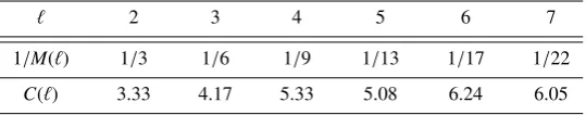
In Table 9.1 we give values for the factor 1/M(`) and the additive constantC(`) that determine the improvements ofRq` overRq for several small extension
Table 9.1 Constants that determine the improvement ofRq` overRq
` 2 3 4 5 6 7
1/M(`) 1/3 1/6 1/9 1/13 1/17 1/22
C(`) 3.33 4.17 5.33 5.08 6.24 6.05
Example 9.2 (Quadratic extensions) LetFq2 =Fq(α) withα2 =ω∈Fq. An
elementβ=b0+b1α,0 can be inverted as
1 b0+b1α
= b0−b1α
b20−b21ω = b0
b20−b21ω− b1
b20−b21ωα. In this case the norm ofβis given explicitly byb2
0−b 2
1ω∈Fq. The inverse of
βthus can be computed in one inversion, two multiplications, two squarings, one multiplication byω, one subtraction and one negation, all inFq, i.e.,Iq2 =
Iq+2Mq+2Sq+M(ω)+subq+negq.
We assume that we multiply Fq2-elements with Karatsuba multiplication,
which costsMq2=3Mq+M(ω)+2addq+2subq. As in the general case above,
we assume that the cost for a full multiplication in the quadratic extension is at leastMq2 ≥3Mq, i.e., we restrict to the average case where both elements have
both of their coefficients different from 0. Thus we can give an upper bound on theI/M-ratio inFq2depending on the ratio inFqas
Rq2 =Iq2/Mq2≤(Iq/3Mq)+2=Rq/3+2,
where we roughly assume that Iq2 ≤ Iq+6Mq. This bound shows that for
Rq > 3 the ratio becomes smaller inFq2. For large ratios in Fq it becomes
roughlyRq/3.
Example 9.3 (Cubic extensions) LetFq3 =Fq(α) withα3 =ω∈Fq. Similar
to the quadratic case we can invertβ=b0+b1α+b2α2∈F∗q3by
1 b0+b1α+b2α2
= b
2
0−ωb1b2
N(β) +
ωb2 2−b0b1
N(β) α+ b2
1−b0b2
N(β) α
2
withN(β)=b30+b31ω+b32ω2−3ωb0b1b2. We start by computingωb1andωb2
as well asb2 0andb
2
1. The terms in the numerators are obtained by a two-way
Karatsuba multiplication and additions and subtractions via 3Mq computing
b0b2, ωb1b2 and (ωb2+b0)(b2+b1). The norm can be computed by three
more multiplications and two additions. Thus the cost for the inversion isIq3=
done inMq3 =6Mq+2M(ω)+9addq+6subq. We useMq3 ≥6Mq, assume
Iq3≤Iq+18Mqand obtain
Rq3=Iq3/Mq3 ≤(Iq/Mq)/6+3=Rq/6+3.
Inversions in towers of field extensions
Baktir and Sunar [7] introduce optimal tower fields as an alternative for optimal extension fields, where they build a large field extension as a tower of small extensions instead of one big extension. They describe how to use the above inversion technique recursively by passing down the inversion in the tower, finally arriving at the base field. They show that this method is more efficient than computing the inversion in the corresponding large extension with the Itoh-Tsujii inversion directly. For towers of field extensions of degree two and three as those occurring in pairing-friendly fields, the inversion can be done using the two examples given above.
9.2.4 Simultaneous inversions
The inverses of sfield elementsa1, . . . ,as can be computed simultaneously
with Montgomery’s well-known inversion-sharing trick [52, Section 10.3.1.] at the cost of one inversion and 3(s−1) multiplications. It is based on the following idea: to compute the inverse of two elementsaandb, one computes their productaband its inverse (ab)−1. The inverses ofaandbare then found bya−1=b·(ab)−1andb−1=a·(ab)−1, with an overall cost of just one inversion
and three multiplications.
In general, forselements one first computes the productsci = a1· · · · ·ai
for 2≤ i ≤ swiths−1 multiplications and invertscs. Then we havea−s1 =
cs−1c−s1. We geta
−1
s−1 byc
−1
s−1 = c
−1
s as anda−s−11 = cs−2c−s−11 and so forth (see
[24, Algorithm 11.15]), where we need 2(s−1) more multiplications to get the inverses of all elements.
Since this method works for general field elements, i.e., it is not restricted to a specific extension degree, we leave out the indices in the notation of the inversion and multiplication costs and their ratio. The cost forsinversions is replaced byI+3(s−1)M. LetRavg,sdenote the ratio of the cost ofsinversions
to the cost ofsmultiplications. It is bounded above by
Ravg,s=I/(sM)+3(s−1)/s≤R/s+3,
i.e., when the numbersof elements to be inverted grows, the ratioRavg,sgets
the inversion method described above in Section 9.2.3 on page 10 might lead to anI/M-ratio that already is less than 3. In this case using the sharing trick at the highest level of the field extension would make the average ratio worse. But a combination of both methods, such as reducing the inversions down to the ground field and sharing them there, can further increase efficiency.
9.3 A
ffi
ne coordinates for pairing computation
The previous section elaborated on two techniques that achieve a low inver-sion to multiplication cost ratio, namely working in exteninver-sion fields and doing several inversions at once if possible. There exist scenarios in which one of the two or both techniques can be applied and lead to affine coordinates being the most efficient choice. Affine coordinates are useful for curve operations in the groupG0
2including those needed in the Miller loop, whenever a
pairing-friendly curve is chosen such that G02 is defined over an extension field of larger degree. This might occur for high security pairings or whenever high-degree twists cannot be used. The second technique of simultaneous inversion becomes possible whenever several pairings or a product of several pairings is computed such that inversions can be synchronized and be done simulta-neously. This section states the costs for the doubling and addition steps in Miller’s algorithm for affine coordinates and explains use cases of the above two techniques for achieving low inversion cost.
9.3.1 Costs for doubling and addition steps
We begin by describing the evaluation of line functions in affine coordinates for ate-like pairings as in Section 9.1.2 on page 6, i.e., a pointPonE,P,O,
is given by two affine coordinates asP = (xP,yP). Let R1,R2,S ∈ E with
R1 ,−R2andR1,R2,S ,O. Then the function of the line throughR1andR2
(tangent toEifR1=R2) evaluated atS is given by
lR1,R2(S)=yS −yR1−λ(xS −xR1),
whereλ=(3x2
R1+a)/2yR1ifR1 =R2andλ=(yR2−yR1)/(xR2−xR1) otherwise.
The valueλis also used to computeR3=R1+R2onEbyxR3=λ
2−x
R1−xR2
and yR3 = λ(xR1 −xR3)−yR1. If R1 = −R2, then we have xR1 = xR2 and
lR1,R2(S)=xS −xR1.
Let the notation be as described in Section 9.1.2, in particular we use a twist E0of degreedto represent the groupG
2by the groupG02. Lete=k/d, then
G02 = E0(Fqe)[r]. Let P ∈ G1,R0,Q0 ∈ G0
2 and letR = ψ(R
Furthermore, we assume that the field extensionFqk is given byFqk =Fqe(α) whereα∈Fqkis the same element as the one defining the twistE0, and we have
αd =ω∈
Fqe. This means that each element inFqk is given by a polynomial of degreed−1 inαwith coefficients inFqe and the twisting isomorphismψmaps (x0,y0) to (α2x0, α3y0).
Doubling steps in affine coordinates
We need to compute
lR,R(P)=yP−α3yR0−λ(xP−α2xR0)=yP−αλ0xP+α3(λ0xR0−yR0)
andR03=[2]R0, wherexR0
3=λ
02−2x
R0andyR0
3 =λ
0(x
R0−xR0
3)−yR
0. We have
λ0=(3x2
R0+a/α4)/2yR0andλ=(3x2
R+a)/2yR=αλ0. Note that [2]R0,Oin
the pairing computation.
The slopeλ0can be computed withI
qe+Mqe+Sqe +4addqe, assuming that we compute 3x2R0and 2yR0by additions. To compute the double ofR0from the
slopeλ0, we need at mostM
qe+Sqe+4subqe. We obtain the line function value with a cost ofeMqto computeλ0xPandMqe+subqe+negqeford∈ {4,6}. When d=2, note thatα2=ω∈
Fqeand thus we need (k/2)Mq+Mqk/2+M(ω)+2subqk/2
for the line.
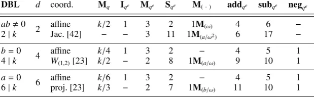
We summarize the operation counts in Table 9.2 on page 16. We restrict to even embedding degree and 4 |kforb = 0 as well as to 6 | kfora = 0 be-cause these cases allow using the maximal-degree twists and are likely to be used in practice. We compare the affine counts to costs of the fastest formu-las using projective coordinates taken from [42] and [23]. For an overview of the most efficient explicit formulas known for elliptic-curve operations see the Explicit-Formulas Database [11]. We transfer the formulas in [42] to the ate pairing using the trick in [23] where the ate pairing is computed entirely on the twist. In this setting we assume field extensions are constructed in a way that favors the representation of line function values. This means that the twist isomorphism can be different from the one described in this chapter. Still, in the cased=2, evaluation of the line function cannot be done inkMq; instead
two multiplications inFqk/2 need to be done (see also the discussion in the
re-spective sections of [23]). Furthermore, we assume that all precomputations are done as described in the above papers and small multiples are computed by additions.
Addition steps in affine coordinates
The line function value has the same shape as for doubling steps. Note that we can replaceR0byQ0in the line and compute
Table 9.2 Operation counts for the doubling step in the ate-like Miller loop omitting1Sqk+1Mqk. The elements a,b∈Fqare the curve coefficients, k is the embedding degree with respect to the prime subgroup order r, and d is the
degree of the twist such that the group G02is defined overFqe where e=k/d.
DBL d coord. Mq Iqe Mqe Sqe M(·) addqe subqe negqe
ab,0 2 affine k/2 1 3 2 1M(ω) 4 6 −
2|k Jac. [42] − − 3 11 1M(a/ω2) 6 17 −
b=0
4 affine k/4 1 3 2 − 4 5 1
4|k W(1,2)[23] k/2 − 2 8 1M(a/ω) 9 10 1
a=0
6 affine k/6 1 3 2 − 4 5 1
6|k proj. [23] k/3 − 2 7 1M(b/ω) 11 10 1
andR0
3 =R
0+Q0, wherex
R0
3 =λ
02−x
R0−xQ0andyR0
3 =λ
0(x
R0−xR0
3)−yR
0.
The slopeλ0now is different, namelyλ0 =(y
R0 −yQ0)/(xR0−xQ0). Note that
R0=−Q0does not occur when computing Miller function values of degree less thanr. The cost for doing an addition step is the same as that for a doubling step, except that the cost to compute the slopeλ0is nowIqe+Mqe+2subqe.
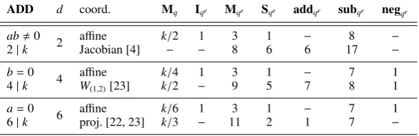
Table 9.3 compares the costs for affine addition steps to those in projective coordinates. Again, we take these operation counts from the literature (see [4, 23, 22] for the explicit formulas and details on the computation). Concerning the field and twist representations and line function evaluation, similar remarks as for doubling steps apply here.
The multiplication withωin the cased=2 can be done as a precomputation, sinceQ0is fixed throughout the pairing algorithm. Since other formulas do not have multiplications by constants, we omit this column in Table 9.3.
Affine versus projective
Doubling and addition steps for computing pairings in affine coordinates in-clude one inversion inFqe per step. The various projective formulas avoid the inversion, but at the cost of doing more of the other operations. How much higher these costs are exactly, depends on the underlying field implementation and the ratio of the costs for squaring to multiplication.
A rough estimate of the counts in Table 9.3 shows that the cost traded for the inversion in the projective addition formulas is equivalent to at least several
Table 9.3 Operation counts for the addition step in the ate-like Miller loop omitting1Mqk. The elements a,b∈Fqare the curve coefficients, k is the embedding degree with respect to the prime subgroup order r, and d is the degree of the twist such that the group G02is defined overFqewhere e=k/d.
ADD d coord. Mq Iqe Mqe Sqe addqe subqe negqe
ab,0 2 affine k/2 1 3 1 − 8 −
2|k Jacobian [4] − − 8 6 6 17 −
b=0
4 affine k/4 1 3 1 − 7 1
4|k W(1,2)[23] k/2 − 9 5 7 8 1
a=0
6 affine k/6 1 3 1 − 7 1
6|k proj. [22, 23] k/3 − 11 2 1 7 −
function is chosen), the traded cost in the doubling case is the most relevant to consider.
The subsection concludes with two examples that give specific upper bounds onIqe such that affine coordinates are more efficient than projective ones.
Example 9.4 Let ab , 0, i.e., d = 2. The cost that has to be weighed
against the inversion cost for a doubling step is 9Sqk/2−(k/2)Mq+M(a/ω2)−
M(ω)+2addqk/2+11subqk/2. Clearly, (k/2)Mq <Sqk/2, and we assumeM(ω) ≈ M(a/ω2) and addqk/2 ≈ subqk/2. We see that if an inversion costs less than
8Sqk/2+13addqk/2, then affine coordinates are better than Jacobian.
Example 9.5 In the casea =0,d =6, similar to the previous example, we deduce that if an inversion inFqk/6is less than 5Sqk/6−Mqk/6+(k/6)Mq+M(b/ω)+
12addqk/6, then affine coordinates beat the projective ones.
In order to fully assess the effect of using affine instead of projective coor-dinates, one needs to know the exact cost that is traded for the inversion. This strongly depends on the specific algorithms chosen to implement the opera-tions in the extension fields. For example, the relative costs between multipli-cations and squarings can differ significantly. Commonly used values in the literature areSq = Mq or Sq = 0.8Mq whenq is a prime, see [11]. Using
Karatsuba multiplication and squaring in a quadratic extension leads to a ratio ofSq2 ≈(2/3)Mq2. Therefore, we do not specify these costs any further and
9.3.2 Working over extension fields
This subsection illustrates the usefulness of affine coordinates when the exten-sion degreeeis relatively large.
To implement pairings at a given security level, on the one hand one needs to find a pairing-friendly elliptic curve such thatrandqkhave a certain minimal size (e.g. given by current estimates for the runtimes of algorithms to solve the ECDLP). On the other hand, for efficiency it is desirable that they are not much larger than necessary. For a pairing-friendly elliptic curveEoverFqwith
embedding degreekwith respect to a prime divisorr|#E(Fq), we define the ρ-value ofEasρ=log(q)/log(r). This value is a measure of the base field size relative to the size of the prime-order subgroup on the curve. The valueρkis the ratio of the sizes ofqkandr. For a given curve the valueρkdescribes how well security is balanced between the curve groups and the finite field group.
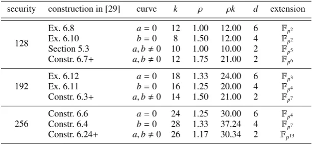
An overview of construction methods for pairing-friendly elliptic curves is given in [29]. In Table 9.4, we list suggestions for curve families by their con-struction in [29] for high-security levels of 128, 192, and 256 bits. The last column in Table 9.4 shows the field extensions in which inversions are done to compute the line function slopes. We not only give families of curves with twists of degree 4 and 6, but also more generic families such that the curves only have a twist of degree 2. Of course, in the latter case the extension field, in which inversions for the affine ate pairing need to be computed, is larger than when dealing with higher-degree twists. Because curves with twists of degree 4 and 6 are special (they have j-invariants 1728 and 0), there might be reasons to choose the more generic curves. Note that curves from the given constructions are all defined over prime fields. Therefore we use the notation Fpin Table 9.4.
Remark The conclusion to underline from the discussion in this section, is that, using the improved inversions in towers of extension fields described here, there are at least two scenarios where most implementations of the ate pairing would be more efficient using affine coordinates.
Table 9.4 Extension fields for which inversions are needed when computing ate-like pairings for different examples of pairing-friendly curve families
suitable for the given security levels.
security construction in [29] curve k ρ ρk d extension
128
Ex. 6.8 a=0 12 1.00 12.00 6 Fp2
Ex. 6.10 b=0 8 1.50 12.00 4 Fp2
Section 5.3 a,b,0 10 1.00 10.00 2 Fp5
Constr. 6.7+ a,b,0 12 1.75 21.00 2 Fp6
192
Ex. 6.12 a=0 18 1.33 24.00 6 Fp3
Ex. 6.11 b=0 16 1.25 20.00 4 Fp4
Constr. 6.3+ a,b,0 14 1.50 21.00 2 Fp7
256
Constr. 6.6 a=0 24 1.25 30.00 6 Fp4
Constr. 6.4 b=0 28 1.33 37.24 4 Fp7
Constr. 6.24+ a,b,0 26 1.17 30.34 2 Fp13
5subq7extra for a doubling (and an extra 6Mq7+4Sq7+7addq7+subq7for an
addition step). In most implementations of the base field arithmetic, the cost of these 16 or 17 operations in the extension field would outweigh the cost of one improved inversion in the extension field.
When special high-degree twists are not being used.In this scenario there are two reasons why affine coordinates will be better under most circumstances. First, the costs for doubling and addition steps given in the first lines of Ta-bles 9.2 and 9.3 for degree-2 twists are not nearly as favorable towards pro-jective coordinates as the formulas in the case of higher degree twists. For degree-2 twists, both the doubling and addition steps require roughly at least 9 extra squarings and 13 or 15 extra field extension additions or subtractions for the projective formulas. Second, the degree of the extension field where the operations take place is larger. See the bottom row for each security level in Table 9.4, so we have extension degree 6 for 128-bit security up to extension degree 13 for 256-bit security.
9.3.3 Simultaneous inversions in pairing computation
This subsection discusses different scenarios, in which the simultaneous inver-sion technique from Section 9.2.4 on page 13 can be applied and might lead to a low-enoughI/Mratio to favor affine coordinates.
Sharing inversions in a single pairing computation
coordi-nates. They suggest postponing addition steps in the double-and-add algorithm to exploit the inversion sharing. In order to do that, the double-and-add algo-rithm must be carried out by going through the binary representation of the scalar from right to left. First, all doublings are carried out and the points that will be used to add up to the final result are stored. When all these points have been collected, several additions can be done at once, sharing the computation of inversions among them.
Miller’s algorithm can also be done from right to left. The doubling steps are computed without doing the addition steps. The required field elements and points are stored in lists and addition steps are done in the end. The algorithm is summarized in Algorithm 3. Unfortunately, addition steps cost much more than in the conventional left-to-right algorithm as it is given in Algorithm 2 on page 7. In the right-to-left version, each addition step in line 10 needs a generalFqk-multiplication and a multiplication with a line function value. The conventional algorithm only needs a multiplication with a line. These huge costs cannot be compensated for by using affine coordinates with the inversion-sharing trick.
Algorithm 3Right-to-left version of Miller’s algorithm with postponed addi-tion steps for evenkand ate-like pairings
Input: Q0∈G0
2,P∈G1,m=(ml−1,ml−2, . . . ,m0)2,ml−1=1 Output: fm,ψ(Q0)(P) representing a class inF∗
qk/(F ∗
qk)
r
1: R0←Q0, f ←1, j←0
2: forifrom 0 to`−1do
3: if(mi=1)then
4: AR0[j]←R0, Af[j]← f, j← j+1
5: end if
6: f ← f2·l
ψ(R0),ψ(R0)(P), R0←[2]R0
7: end for
8: R0←AR0[0], f ←Af[0]
9: for(j←1; j≤h(m)−1;j+ +)do
10: f ← f·Af[j]·lψ(R0),ψ(A
R0[j])(P), R
0←R0+A
R0[j]
11: end for
12: return f
Parallelizing a single pairing
to compute a single pairing by doing addition steps in parallel on two different cores. They divide the lists with the saved function values and points into two halves and compute two intermediate values which are in the end combined in a single addition step. For their specific implementation, they conclude that this is not faster than the conventional non-parallel algorithm. Still, this idea might be useful for two or more cores, in case multiple cores can be used with less overhead. It is straightforward to extend this algorithm to more cores.
The parallelized algorithm can be combined with the shared inversion trick when doing the addition steps in the end. The improvements achieved by this approach strongly depend on the Hamming weight of the valuemin Miller’s algorithm. If it is large, then savings are large, while for very sparsemthere is almost no improvement. Therefore, when it is not possible to choosemwith low Hamming weight, combining the parallelized right-to-left algorithm for pairings with the shared inversion trick can speed up the computation. The communication overhead in order to gather data from intermediate computa-tions on different cores to compute the inverse at one core imposes a non-trivial performance penalty and it remains to be seen whether this approach is worth-while. Grabher et al. [34] note that when multiple pairings are computed, it is better to parallelize by performing one pairing on each core.
Multiple pairings and products of pairings
Many protocols involve the computation of multiple pairings or products of pairings. For example, multiple pairings need to be computed in the searchable encryption scheme of Boneh et al. [15]; and the non-interactive proof systems proposed by Groth and Sahai [37] need to check pairing product equations. In these scenarios, we propose sharing inversions when computing pairings with affine coordinates. In the case of products of pairings, this has already been proposed and investigated by Scott [57, Section 4.3] and Granger and Smart [36]. See also the more recent work [58] by Scott.
Multiple pairings
Assume we want to computespairings on pointsQ0
i andPi, i.e., a priori we
havesMiller loops to compute fm,ψ(Q0
So when computing sufficiently many pairings so that the average cost of an inversion is small enough, using the sliced-Miller approach with inversion sharing in affine coordinates is faster than using the projective coordinates ex-plicit formulas described in Section 9.3.1 on page 14.
Products of pairings
For computing a product of pairings, more optimizations can be applied, in-cluding the above inversion-sharing. Scott [57, Section 4.3] suggests using affine coordinates and sharing the inversions for computing the line function slopes as described above for multiple pairings. Furthermore, since the Miller function of the pairing product is the product of the Miller functions of the sin-gle pairings, in each doubling and addition step the line functions can already be multiplied together. In this way, we only need one intermediate variable f and only one squaring per iteration of the product Miller loop. Of course in the end, there is only one final exponentiation on the product of the Miller function values. Granger and Smart [36] show that by using these optimizations the cost for introducing an additional ate pairing to the product can be as low as 13% of the cost of a single ate pairing.
9.4 The double-add operation and parabolas
This section consists largely of lightly edited material from Sections 3, 5, and 6 of [27]. In [27], an improvement to the double-and-add operation on an elliptic curve was introduced, and a related idea was applied to improve the analogous operation in pairing computations on elliptic curves. In affine coordinates, the technique allows one to perform a doubling and an addition, 2P+Q, on an elliptic curveEusing only 1M+2S+2I(plus an extra squaring whenP=Q). This is achieved as follows: to compute 2P+Q, where P = (x1, y1) and
Q=(x2, y2), first find (P+Q), but omit itsy-coordinate since it is not needed
for the next stage. This saves one field multiplication. Next compute (P+Q)+P. This way, two point additions are performed while saving one multiplication. This trick also works whenP=Q, i.e., when tripling a point.
9.4.1 Description of the algorithm
Suppose P = (x1, y1) and Q = (x2, y2) are distinct points on E different
from O, and x1 , x2. The details for other cases are given in Figure 1 of
that the pointP+Qis then given by (x3, y3), where x3 =λ21−x1−x2and
y3=(x1−x3)λ1−y1withλ1 =(y2−y1)/(x2−x1).
To add (P+Q) toP, add (x1, y1) to (x3, y3) using the above rule (assuming
x3 , x1). The result has coordinates (x4, y4), where x4 = λ22 −x1−x3 and
y4=(x1−x4)λ2−y1withλ2 =(y3−y1)/(x3−x1).
The computation ofy3can be omitted because it is used only in the
compu-tation ofλ2, which can be computed without knowingy3as
λ2 =−λ1−2y1/(x3−x1).
Omitting they3 computation saves one field multiplication. Eachλ2 formula
requires a field division, so the overall saving is this one field multiplication. This trick can also be applied to save one multiplication when computing 3P, the triple of a pointP ,O, where theλ2computation will need the slope of
a line through two distinct points 2PandP. It can be used twice to save two multiplications when computing 3P+Q=((P+Q)+P)+P. Thus 3P+Qcan be computed using one multiplication, three squarings, and three divisions. Such a sequence of operations would be performed repeatedly if an exponent were written in ternary form and left-to-right exponentiation were used. Ternary re-presentation performs worse than binary rere-presentation for large random expo-nentsk, but the operation of triple and add was explored further in the context of double-base chains in [21, Section 5].
9.4.2 Application to scalar multiplication
The above double-and-add operation can be applied to scalar multiplications on an elliptic curve in affine coordinates. In the naive left-to-right method of binary exponentiation, the double-and-add trick can be applied repeatedly at each stage of the computation. More efficient variants could use a combination of the left-to-right or right-to-leftm-ary exponentiation with sliding window methods, addition-subtraction chains, signed representations, etc. When using affine coordinates, the double-and-add trick can be used on top of these meth-ods form=2 to obtain savings, depending upon the window size that is used. Note that we discuss the double-and-add technique in a historic manner and neglect the protection of scalar multiplication against side channels such as making sure that the algorithm runs in constant time.
Another application, in which the double-and-add operation occurs more frequently than in single scalar multiplication is multi-exponentiation, for ex-ample a simultaneous three-fold scalar multiplicationk1P1+k2P2+k3P3, where
the three exponentsk1,k2, andk3have approximately the same length. One
P1,P3,P3+P1,P3+P2,P3+P2+P1.Subsequently it uses one elliptic curve
doubling followed by the addition of a table entry, for each bit in the exponents [51]. For random scalarskiand a binary scalar decomposition, about 7/8 of the
doublings will be followed by an addition other thanO.
9.4.3 Application to pairings
The double-and-add technique can be extended to the function evaluation in Miller’s algorithm and thus can be applied to pairing computation as well. The key observation is that one can replace consecutive evaluations of line functions by the evaluation of a parabola, and thus obtain an analogue to the double-and-add operation in the form of a Miller formula.
Using the double-and-add trick with parabolas
We use notation as in the paragraph on Miller’s algorithm in Section 9.1.2 on page 4. For two integersb,c, instead of computing f2b+c,P(Q) and [2b+c]P
from (fb,P(Q),[b]P) and (fc,P(Q),[c]P) via f2b,P(Q) = fb2,P(Q)g[b]P,[b]P and
[2]([b]P), and then f2b+c,P(Q)= f2b,P(Q)fc,P(Q)g[2b]P,[c]Pand [2b]P+[c]P, we
now describe an alternative approach that computes the result directly, produc-ing only the x-coordinate of the intermediate point [b]P+[c]P. To combine the two steps, one constructs a parabola through the points [b]P, [b]P, [c]P,
−[2b+c]P.
To form f2b+c,P(Q), combine forming fb+c,P(Q) with fb+c+b,P(Q) as follows.
We omit the notation for evaluation at Qand simply write f2b+cetc. and use
the notationlPfor the vertical line functionlP,−PthroughPand−P. We have
f2b+c,P= fb+c,P·fb,P·g[b+c]P,[b]P
=(fb,P·fc,P·g[b]P,[c]P)·(fb,P·g[b+c]P,[b]P)
= f
2
b,P· fc,P
l[2b+c]P
·l[b]P,[c]P·l[b+c]P,[b]P
l[b+c]P .
Now, one can replace the second fraction l[b]P,[c]P ·l[b+c]P,[b]P/l[b+c]P by the
parabola whose formula is given in the next paragraph.
Equation for the parabola
If R andS are points on E, then there is a (possibly degenerate) parabolic equation passing throughRtwice (i.e., tangent atR) and also passing through S and−[2]R−S. Using the notationR = (x1, y1) and S = (x2, y2) with
R+S =(x3, y3) and 2R+S =(x4,y4), a formula for this parabola is
(y+y3−λ1(x−x3))(y−y3−λ2(x−x3))
x−x3
The left half of the numerator of (9.4) is a line passing throughR,S, and−R−S whose slope isλ1. The second half of the numerator is a line passing through
R+S,R, and−[2]R−S, whose slope isλ2. The denominator is a (vertical) line
throughR+S and−R−S. The quotient has zeros atR,R,S,−[2]R−S and a pole of order four atO.
One can simplify Equation (9.4) by expanding it in powers ofx−x3, using
the Weierstrass equation forEto eliminate references toy2andy23. y2−y23
x−x3
−λ1(y−y3)−λ2(y+y3)+λ1λ2(x−x3)
=x2+xx3+x23+a+λ1λ2(x−x3)−λ1(y−y3)−λ2(y+y3) (9.5)
=x2+(x3+λ1λ2)x−(λ1+λ2)y+(x23+a−λ1λ2x3+(λ1−λ2)y3).
Knowing that (9.5) passes throughR = (x1,y1), one succinct formula for the
parabola is
(x−x1)(x+x1+x3+λ1λ2)−(λ1+λ2)(y−y1). (9.6)
In the previous section we can now replacel[b]P,[c]P ·l[b+c]P,[b]P/l[b+c]P by the
parabola (9.6) withR = [b]PandS = [c]P. Formula (9.6) for the parabola does not referencey3and is never identically zero since itsx2coefficient is 1.
The following example shows how in the case of affine coordinates, the double-and-add operation can help to make the pairing algorithm more effi -cient.
Example 9.6 Assume that we are computing an ate-like pairing in the same setting as in Section 9.3.1 on page 14. Letab , 0, i.e.,d = 2, letkbe even
such that we can use denominator elimination, and note thatω = α2. Now, assume that we are at a position in the Miller loop, where we are computing a doubling step followed by an addition step. This means that the two steps compute f[2]R0+Q0,ψ(Q0)(P) from fR0,ψ(Q0)(P) andR0. Let us first analyse the cost
when doing this the usual way. We simply add the costs for doubling and addi-tion from Tables 9.2 on page 16 and 9.3 on page 17, respectively. The resulting cost iskMq+2Iqk/2+6Mqk/w+3Sqk/2+1M(ω)+4addqk/2+14subqk/2plus the
squaring costSqk for the standard Miller loop squaring and two multiplications 2Mqk with line functions, which are regular field multiplications inFqk because line functions are not sparse in this case.
2M(ω)+M(ω2)+5addqk/2+8subqk/2+addq+subq. Overall, the parabola
tech-nique savesMqk+(k/2)Mqk/2+Sqk/2, clearly theaddandsubcosts are lower,
but it uses two more multiplications by ωandω2, respectively. In this spe-cific setting, the parabola method is indeed more efficient than the standard Miller loop with only doubling and addition steps. This effect becomes more pronounced for larger embedding degrees.
9.5 Squared pairings
For applications to cryptography, the idea of using the squared Weil or Tate pairing instead of the usual pairings was introduced in [28]. Peter was very fond of the idea of squared pairings. The denominator cancellation, which im-proves efficiency, was one very nice consequence, but that was also achieved independently in a different way in [8, 9]. However, an often unrecognized part of the history is that the squared Weil pairing may be viewed as a precursor to the definition of the ate pairing and optimal pairings which are in the same vein as the squared pairing. Namely, those more recent definitions consider a higher power of the Tate pairing and achieve greater efficiency by reducing the Miller loop length. The following exposition of the squared Weil and Tate pairings is a lightly edited version of Sections 2 and 3 from [28].
9.5.1 The squared Weil pairing
The squared pairing idea was introduced in [28] as a construction of new pair-ings, called thesquared Weil pairingandsquared Tate pairing. An analogous pairing for hyperelliptic curves was also introduced. In each case, a direct for-mula for evaluating the pairing was given, along with proofs that the values coincide with the value of the original pairing (Weil or Tate) squared. Here we present only the construction of the new pairing, and omit the proofs of cor-rectness. These alternate pairings had the advantage of being more efficient to compute than Miller’s algorithm for the original Weil and Tate pairings. The squared pairing also has the advantage that it is guaranteed to output the correct answer and does not depend on inputting a randomly chosen point. In contrast, Miller’s algorithm may restart, since the randomly chosen point can cause the algorithm to fail.
Algorithm forer(P,Q)2
Given twor-torsion pointsPandQonE, we want to computeer(P,Q)2. Start
in the chain is a sum or difference of two earlier elements, until anrappears. Well-known techniques give a chain of lengthO(log(r)). For each j in the addition-subtraction chain, form a tupletj=[[j]P,[j]Q,nj,dj] such that
nj
dj
= fj,P(Q) fj,Q(−P)
fj,P(−Q) fj,Q(P)
. (9.7)
Start witht1=[P,Q,1,1]. Giventjandtk, the following procedure getstj+k.
1 Compute the points [j]P+[k]P=[j+k]Pand [j]Q+[k]Q=[j+k]Q. 2 Find coefficients of the linel[j]P,[k]P(X)=c0+c1x(X)+c2y(X).
3 Find coefficients of the linel[j]Q,[k]Q(X)=c00+c01x(X)+c02y(X).
4 Set
nj+k=njnk(c0+c1x(Q)+c2y(Q)) (c00+c
0
1x(P)−c
0
2y(P)),
dj+k=djdk(c0+c1x(Q)−c2y(Q)) (c00+c
0
1x(P)+c
0
2y(P)).
A similar construction givestj−kfromtjandtk. The vertical lines through [j+
k]Pand [j+k]Qdo not appear in the formulas fornj+kanddj+k, because the
contributions fromQand−Q(or fromPand−P) are equal. When j+k=r, this simplifies tonj+k=njnkanddj+k=djdk, sincec2andc02will be zero.
Whennranddrare non-zero, then the computation
nr
dr
= fr,P(Q) fr,Q(−P)
fr,P(−Q) fr,Q(P)
has been successful, and we have the correct output. If, however,nr ordr is
zero, then some factor such asc0+c1x(Q)+c2y(Q) must have vanished. That
line was chosen to pass through [j]P, [k]P, and−[j+k]P, for some jandk. It does not vanish at any other point on the elliptic curve. Therefore this factor can vanish only ifQ=[j]PorQ=[k]PorQ=−[j+k]P. In all of these cases Qwill be a multiple ofP, ensuringer(P,Q)=1.
Overall, the squared Weil pairing advances fromtiandtjtoti+jwith 12 field
multiplications and 2 field divisions in the generic case, compared to 18 field multiplications and 2 field divisions for Miller’s general method. Wheni= j, each algorithm needs 2 additional field multiplications due to the elliptic curve doublings.
9.5.2 The squared Tate pairing
AssumeP∈ E(Fq)[r], andQ∈ E(Fqk), with neither being the identity andP not equal to a multiple ofQ. Define
vr(P,Q) :=
fr,P(Q)
fr,P(−Q)
!(qk−1)/r
where fr,P is as above, and callvr the squared Tate pairing. To justify this
terminology, it was shown in [28] thatvr(P,Q)=tr(P,Q)2.
Algorithm forvr(P,Q)
Given anr-torsion pointP on E and a point Qon E, we want to compute vr(P,Q). As before, start with an addition-subtraction chain forr. For eachjin
the addition-subtraction chain, form a tupletj=[[j]P,nj,dj] such that
nj
dj
= fj,P(Q)
fj,P(−Q)
. (9.8)
Start witht1=[P,1,1]. Giventjandtk, the following procedure getstj+k.
1 Compute the points [j]P+[k]P=[j+k]P.
2 Find the line functiong[j]P,[k]P(X)=c0+c1x(X)+c2y(X).
3 Set
nj+k=nj·nk·(c0+c1x(Q)+c2y(Q)),
dj+k=dj·dk·(c0+c1x(Q)−c2y(Q)).
A similar construction givestj−kfromtjandtk. The vertical lines through [j+
k]P and [j+k]Q do not appear in the formulas fornj+k and dj+k, because
the contributions fromQand−Qare equal. When j+k=r, one can further simplify this tonj+k =nj·nkanddj+k =dj·dk, sincec2 will be zero. When
nranddrare non-zero, then the computation of (9.8) with j=ris successful,
and after raising to the (qk−1)/r-th power, we have the correct output. If somenr ordrwere zero, then some factor such asc0+c1x(Q)+c2y(Q) must
Bibliography
[1] D. F. Aranha, P. S. L. M. Barreto, P. Longa, and J. E. Ricardini. The realm of the pairings. In T. Lange, K. Lauter, and P. Lisonek, editors,SAC 2013: 20th Annual International Workshop on Selected Areas in Cryptography, volume 8282 ofLecture Notes in Computer Science, pages 3–25. Springer, Heidelberg, Aug. 2014. (Cited on pages 2 and 9.)
[2] D. F. Aranha, L. Fuentes-Castañeda, E. Knapp, A. Menezes, and F. Rodríguez-Henríquez. Implementing pairings at the 192-bit security level. In M. Abdalla and T. Lange, editors,Pairing-Based Cryptography – Pairing 2012, volume 7708 ofLecture Notes in Computer Science, pages 177–195. Springer, 2012. (Cited on page 2.)
[3] D. F. Aranha, K. Karabina, P. Longa, C. H. Gebotys, and J. López. Faster explicit formulas for computing pairings over ordinary curves. In K. G. Paterson, editor,
Advances in Cryptology – EUROCRYPT 2011, volume 6632 ofLecture Notes in Computer Science, pages 48–68. Springer, Heidelberg, May 2011. (Cited on pages 2 and 9.)
[4] C. Arène, T. Lange, M. Naehrig, and C. Ritzenthaler. Faster computation of the Tate pairing. Journal of Number Theory, 131(5):842–857, 2011. (Cited on pages 16 and 17.)
[5] R. M. Avanzi, H. Cohen, C. Doche, G. Frey, T. Lange, K. Nguyen, and F. Ver-cauteren.Handbook of Elliptic and Hyperelliptic Curve Cryptography. Chapman & Hall/CRC Press, 2005. (Cited on page 30.)
[6] D. V. Bailey and C. Paar. Efficient arithmetic in finite field extensions with ap-plication in elliptic curve cryptography. Journal of Cryptology, 14(3):153–176, 2001. (Cited on page 10.)
[7] S. Baktir and B. Sunar. Optimal tower fields. IEEE Transactions on Computers, 53(10):1231–1243, 2004. (Cited on page 13.)
[8] P. S. L. M. Barreto, H. Y. Kim, B. Lynn, and M. Scott. Efficient algorithms for pairing-based cryptosystems. In M. Yung, editor,Advances in Cryptology – CRYPTO 2002, volume 2442 ofLecture Notes in Computer Science, pages 354– 368. Springer, Heidelberg, Aug. 2002. (Cited on pages 2, 4, 7, and 26.)
[9] P. S. L. M. Barreto, B. Lynn, and M. Scott. Efficient implementation of pairing-based cryptosystems.Journal of Cryptology, 17(4):321–334, Sept. 2004. (Cited on pages 4, 7, and 26.)
[10] N. Benger and M. Scott. Constructing tower extensions of finite fields for imple-mentation of pairing-based cryptography. In M. A. Hasan and T. Helleseth, edi-tors,Arithmetic of Finite Fields, Third International Workshop, WAIFI 2010, Is-tanbul, Turkey, June 27-30, 2010. Proceedings, volume 6087 ofLecture Notes in Computer Science, pages 180–195. Springer, 2010. (Cited on page 10.)
[11] D. J. Bernstein and T. Lange. Explicit-Formulas Database, 2016. https:// hyperelliptic.org/EFD. (Cited on pages 15 and 17.)
Cryptography, volume 6487 ofLecture Notes in Computer Science, pages 21–39. Springer, Heidelberg, Dec. 2010. (Cited on pages 2 and 9.)
[13] I. F. Blake, G. Seroussi, and N. P. Smart, editors.Elliptic Curves in Cryptography. Cambridge University Press, 1999. (Cited on page 3.)
[14] I. F. Blake, G. Seroussi, and N. P. Smart, editors. Advances in Elliptic Curve Cryptography. Cambridge University Press, 2005. (Cited on page 31.)
[15] D. Boneh, G. Di Crescenzo, R. Ostrovsky, and G. Persiano. Public key encryption with keyword search. In C. Cachin and J. Camenisch, editors,Advances in Cryp-tology – EUROCRYPT 2004, volume 3027 ofLecture Notes in Computer Science, pages 506–522. Springer, Heidelberg, May 2004. (Cited on page 21.)
[16] D. Boneh and M. K. Franklin. Identity-based encryption from the Weil pairing. In J. Kilian, editor,Advances in Cryptology – CRYPTO 2001, volume 2139 of
Lecture Notes in Computer Science, pages 213–229. Springer, Heidelberg, Aug. 2001. (Cited on page 1.)
[17] D. Boneh, E.-J. Goh, and K. Nissim. Evaluating 2-DNF formulas on ciphertexts. In J. Kilian, editor,TCC 2005: 2nd Theory of Cryptography Conference, volume 3378 ofLecture Notes in Computer Science, pages 325–341. Springer, Heidel-berg, Feb. 2005. (Cited on page 1.)
[18] D. Boneh, B. Lynn, and H. Shacham. Short signatures from the Weil pairing. In C. Boyd, editor,Advances in Cryptology – ASIACRYPT 2001, volume 2248 of
Lecture Notes in Computer Science, pages 514–532. Springer, Heidelberg, Dec. 2001. (Cited on page 1.)
[19] D. Boneh, B. Lynn, and H. Shacham. Short signatures from the Weil pairing.
Journal of Cryptology, 17(4):297–319, Sept. 2004. (Cited on page 1.)
[20] D. Boneh, A. Sahai, and B. Waters. Functional encryption: Definitions and chal-lenges. In Y. Ishai, editor,TCC 2011: 8th Theory of Cryptography Conference, volume 6597 ofLecture Notes in Computer Science, pages 253–273. Springer, Heidelberg, Mar. 2011. (Cited on page 1.)
[21] M. Ciet, M. Joye, K. Lauter, and P. L. Montgomery. Trading inversions for multi-plications in elliptic curve cryptography. Des. Codes Cryptography, 39(2):189– 206, 2006. (Cited on page 23.)
[22] C. Costello, H. Hisil, C. Boyd, J. M. González Nieto, and K. K.-H. Wong. Faster pairings on special Weierstrass curves. In H. Shacham and B. Waters, editors,
PAIRING 2009: 3rd International Conference on Pairing-based Cryptography, volume 5671 ofLecture Notes in Computer Science, pages 89–101. Springer, Hei-delberg, Aug. 2009. (Cited on pages 16 and 17.)
[23] C. Costello, T. Lange, and M. Naehrig. Faster pairing computations on curves with high-degree twists. In P. Q. Nguyen and D. Pointcheval, editors,PKC 2010: 13th International Conference on Theory and Practice of Public Key Cryptography, volume 6056 ofLecture Notes in Computer Science, pages 224–242. Springer, Heidelberg, May 2010. (Cited on pages 15, 16, and 17.)
[24] C. Doche.Finite Field Arithmetic, chapter 11 in [5], pages 201–237. CRC press, 2005. (Cited on pages 10 and 13.)
[25] S. Duquesne and G. Frey. Background on Pairings, chapter 6 in [5], pages 115– 124. CRC press, 2005. (Cited on page 3.)