Constraining Fission Yields Using Machine Learning
AmyLovell1,2,∗,ArvindMohan1,3,∗∗,PatrickTalou4,∗∗∗, andMichaelChertkov3,∗∗∗∗
1Center for Nonlinear Studies, Los Alamos National Laboratory, Los Alamos, NM 87545, USA 2Nuclear Physics Group, Theoretical Division, Los Alamos National Laboratory, Los Alamos, NM
87545, USA
3Condensed Matter Physics and Complex Systems Group, Theoretical Division, Los Alamos National
Laboratory, Los Alamos, NM 87545, USA
4Materials and Physical Data Group, X Computational Physics Division, Los Alamos National
Labora-tory, Los Alamos, NM 87545, USA
Abstract.Having accurate measurements of fission observables is important for a variety of applications, ranging from energy to non-proliferation, defense to astrophysics. Because not all of these data can be measured, it is necessary to be able to accurately calculate these observables as well. In this work, we exploit Monte Carlo and machine learning techniques to reproduce mass and kinetic energy yields, for phenomenological models and in a model-free way. We begin with the spontaneous fission of252Cf, where there is abundant
experi-mental data, to validate our approach, with the ultimate goal of creating a global yield model in order to predict quantities where data are not currently available.
1 Introduction
It is important to reliably and consistently calculate fission observables for applications such as energy, non-proliferation, defense, and astrophysics. Often, fission observables are cal-culated independently of one another, leading to inconsistencies within evaluations (recently shown, for example, in [1]). However, now with tools such as CGMF [2], we can form a consistent picture of fission from scission to the emission of prompt neutrons andγrays.
There are many models available to describe single prompt fission observables (e.g. emit-ted neutron energy spectra or neutron average multiplicity). Some of these models calculate fission yields from shape parameterizations of nuclei using fundamental interactions, i.e. [3– 7]; this is typically computationally expensive. However, most are phenomenological and must be tuned individually to reproduce data. While there are many optimization schemes available (including Monte Carlo techniques), machine learning algorithms can, in principle, learn the complex mapping between observables of the same system and different systems, enhancing the calculation of correlated observables and giving more predictive power. Cur-rently, machine learning is still in its infancy in nuclear physics, and only a few examples are available (i.e. [8, 9]).
In this work, we begin with a study of 252Cf observables, focusing first on mass and total kinetic energy yields. Because it spontaneously fissions, a large body of data have been collected, ranging from yields, to multiplicity distributions and correlated observables. It is therefore an ideal case to study a variety of optimization methods and understand the strengths of each before tackling systems where less experimental data is available. The standard optimization method that we discuss has also been studied for252Cf in a previous work [10], giving us a baseline with which to benchmark our results before exploring the more novel machine learning techniques.
This proceedings is organized as follows. In Section 2, we discussed the physical mod-els that are used in this work, followed by the numerical methods in Section 3. We then summarize our results in Section 4 and conclude in Section 5.
2 Theory
Fission is a rich and complex process that can be described using a range of physical models. Here, we only focus on prompt fission, in particular, the emission of prompt neutrons andγ rays from the fission fragments.
2.1 CGMF
To model the decay of the fission fragments and resulting correlations, the Monte Carlo code CGMF, has been developed [2]. The Hauser-Feschbach statistical model is used to follow the decay of the two daughter fission fragments on an event-by-event basis. At each step of the decay, probabilities for emitting neutrons orγrays are calculated. For each decay, the energy and angle of the fission fragments and emitted particles are recorded, enabling the calculation of correlations between various observables.
In order to initialize these decays, yields in mass, charge, total kinetic energy, spin, and parity are required,Y(A,Z,T KE,J,P). Currently, the sum of three Gaussians is used for the mass distribution, the TKE distribution is described by a single Gaussian for each fragment mass, the charge is determined from Wahl systematics [11], the spin distribution is propor-tional to (2J+1)exp(−0.5J(J+1)~2/(αIo(A,Z)T)) (Io(A,Z) being the ground-state moment
of inertia of nucleus (A,Z) andαthe spin cut-offparameter), and the parity is chosen to be positive or negative with equal probability. The total kinetic energy is shared between the two daughter fragments based on an effective temperature ratio between the light and heavy fragments, which can either be constant or mass-dependent.
2.2 Brosa Yield Model
Currently, the models for Y(A) and Y(T KE) in CGMF are uncorrelated. In 1990, Brosa [12] published a model forY(A,T KE) based on separate fission modes or channels which correspond to different families of shapes of the fissioning system: standard (shown to be comprised of three modes, S1, S2, and S3), superlong (SL), and superasymmetric (SX).
For each mode, the yields are described by
Y(A,T KE)=X
m
Ym(A)Ym(T KE|A), (1)
where
Ym(A)=
wm p
8πσ2
m "
exp −(A−A¯m)
2
2σ2
m !
+exp −(A−Acn+A¯m)
2
2σ2
m !#
and
Ym(T KE|A)=
200 T KE !2 exp " 2d max m −dminm
ddec m
−Tm(A)
ddec m
−(d max
m −dminm )2
Tm(A)dmdec #
. (3)
Here,
Tm(A)=
(Zcn/Acn)2(Acn−A)Ae2
T KE −d
min
m , (4)
whereZcnandAcnare the charge and mass of the fissioning system. Each mode,m, has six
free parameters,wm, ¯Am,σm,dmaxm ,dminm ,ddecm , which are, respectively, the weight of the mode,
the mean mass of the heavy fragment, the width of the mass distribution, the most favorable semilength for fission, the minimum semilength below which fission will not occur, and the the length scale for the decay of the exponential. Since the weights describe the relative probabilities of each mode being populated, they must sum to one.
3 Methods
We have been exploring two paths to construct these yields. The first uses more traditional optimization techniques, in particular a Markov Chain Monte Carlo (MCMC). The second uses a machine learning algorithm. These are described below.
3.1 Monte Carlo Methods
First, a Markov Chain Monte Carlo [13] is used to find a best fit for the free parameters in Equations 2 and 3. This is done by exploring parameter space through randomly generated sets of parameters. Each randomly generated parameter set,i, depends on the previous one, i−1, through a Gaussian distributionxi ∼ N(xi−1, x0),whereis a scaling factor, andx0 is a fixed parameter set. Here,x0is the initial parameter set as given by Brosa in [12]. This combination allows flexibility in the step size while keeping the step size appropriate for the scale of each parameter.
Each new parameter set is accepted or rejected based on the criteria
R< exp(−χ 2
i/2)
exp(−χ2
i−1/2)
, (5)
whereR is a random number sampled uniformly in [0,1], andχ2i is theχ2-value of theith parameter set, defined as
χ2=X
j
Ythj −Yexpj σexp Yj 2 . (6)
Here,Yth
j is a calculated yield for a given value of mass and kinetic energy as in Eq. 1,Y
exp
j
is the experimental yield for the same mass and kinetic energy, andσexpY
j is the experimental error onYexpj .
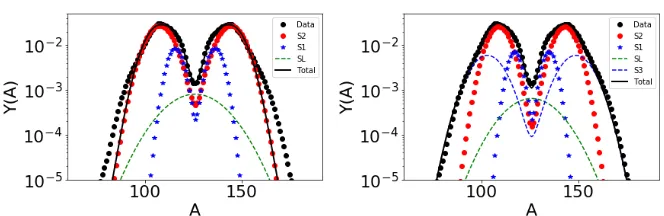
Figure 1.Mass yields when (left) three Brosa modes were fit using the MCMC and when (right) four Brosa modes were fit. Black solid lines show the total fit compared to the experimental data from [15].
3.2 Probabilistic Neural Networks
Neural networks (NN) are a machine learning algorithm that try to learn a complex relation-ship between input and output using a large-scale, data-driven optimization over hundreds of thousands of parameters. The base unit of the network is a neuron, several of which can be arranged in layers (the input and output each comprise a layer), and each neuron has a weight and a bias that are learned. The combination of these layers form the NN. The structure of the layers is driven by the specific application.
In a typical NN, the weights and biases are optimized based on a maximum likelihood es-timation (MLE), which is a deterministic approach and cannot take into account uncertainties in the training data. Inherently, nuclear data contain uncertainties which should be included. In addition, a standard MLE will perform an average over discrepant data sets which may not reflect the confidence in each individual set.
To take this into account, we use a probabilistic machine learning approach - the Mixture Density Network (MDN) [14]. This approach predicts the complex mapping between input and output,y= f(x), as a mixture of Gaussians,
f(x)=α1N(µ1, σ1)+...+αnN(µn, σn). (7)
The values ofαi,µi, andσiare learned by the NN, and the user has control over the number
of Gaussians that are included (as well as the underlying architecture of the NN).
4 Results and Discussion
We began with a MCMC to constrain the Brosa mode parameters for252Cf spontaneous fis-sion yields. First, data from [15] were used to constrain, simultaneously, the Brosa parameters for the S2, S1, and SL modes. We then introduced the S3 mode, rerunning the MCMC for the four modes, and finally included the SX mode as well. The results forY(A) using three and four modes are shown in Fig. 1, along with the contributions of from each of the modes. (The contribution from the SX mode was effectively negligible.)
Nmodes hT KEi(MeV) σT KE(MeV) ν¯
O 185.77 8.97 8.758
3 184.46 10.20 3.956
4 184.16 10.74 3.946
5 184.27 10.71 3.948
5O 185.85 8.85 3.767
Table 1.Observables calculated from CGMF from the default parameterization (O), three, four, and five modes, as well as when five modes were fit to the default yields of CGMF (5O).
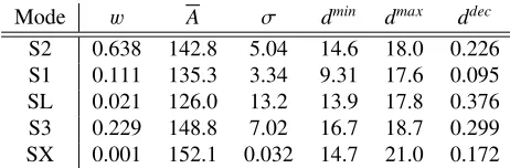
Mode w A σ dmin dmax ddec
S2 0.638 142.8 5.04 14.6 18.0 0.226
S1 0.111 135.3 3.34 9.31 17.6 0.095
SL 0.021 126.0 13.2 13.9 17.8 0.376
S3 0.229 148.8 7.02 16.7 18.7 0.299
SX 0.001 152.1 0.032 14.7 21.0 0.172
Table 2.Brosa parameters corresponding to the CGMF calculation in the last row of Table 1.
modes toY(A,T KE) sampled from the current Gaussian implementation within CGMF. This gives much more accurate results forhT KEiand ¯ν(last row of Table 1). The corresponding Brosa parameters are listed in Table 2.
OncehT KEiand ¯νwere better reproduced, a sensitivity study was performed to determine the linear response of several observables calculated with CGMF to the parameters of the Brosa modes. This response is calculated as
Si j=
xi
0
R0j ∂Rj
∂xi !
x0
, (8)
wherexi0are the best-fit parameters, andR0j are the calculated observables atx0. The deriva-tive in Eq. 8 is calculated at x0 using the three-point midpoint formula. The ratioxi0/R
j
0 is included for normalization. Responses were calculated forhT KEi, σT KE, ¯ν,hν(ν−1)i
(second factorial moment),hν(ν−1)(ν−2)i(third factorial moment), ¯νγ,hνγ(νγ−1)i, and
hνγ(νγ −1)(νγ−2)i;x0were the parameters from the five mode fit, excluding ¯AS L, fixed at
126, andwS L, used to enforce the normalization condition described in Sec. 2.2.
Figure 2 shows the results of these calculations. The most influential parameters aredmaxS2 , dmaxS3 , ¯AS2, and ¯AS3. The twodmaxparameters strongly influence the distributions ofT KEand number of neutrons, while ¯Ahas a reduced - but noticeable - effect on the distribution of the number ofγrays. This is consistent with what was seen in [10] where ¯Aanddmaxof the most
prominent mode (S2) had the largest response. When all five modes were included, the S2 and S3 modes contributed to approximately 80% of the yields; these are also the two modes that cause the most impact on the observables calculated here.
Figure 2.Responses of various observables calculated with CGMF to small changes in the Brosa mode parameters, as defined by Eq. 8.
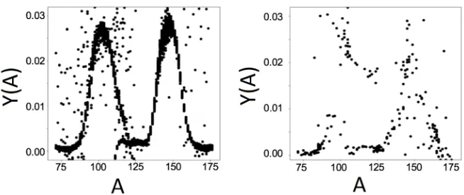
Figure 3.Results of the MDN attempt to learnY(A) for a sparse data set of238Pu(sf) (left) using transfer
learning with252Cf(sf) (right) without transfer learning.
explicitly determined for these parameters. For these reasons, we have also begun to explore machine learning techniques.
In this work, we also explore the suitability of a MDN to estimate fission observables. Although the ultimate goal is to calculate all of the prompt fission observables, we began with mass yields. First, we used a three-layer MDN and train 20 Gaussians on CGMF calcu-lations forY(A) of252Cf spontaneous fission. This method was able to learn the weights and Gaussian parameters to reproduce the inputted simulations.
5 Conclusions
In conclusion, we explored two ways of constraining fission fragment yields, using both para-metric models as well as machine learning techniques. Using a Markov Chain Monte Carlo, we were able to reproduce fission fragment yields for the spontaneous fission of252Cf as a function of mass and total kinetic energy. These yields were implemented into the Hauser-Feschbach Monte Carlo code, CGMF, in order to calculate correlated fission observables. Although the experimental value of ¯νwas not reproduced when fitting to the experimental data of [15], this value was reproduced whenY(A,T KE) sampled from the default version CGMF was used to constrain the Brosa mode parameters. Using not only the yields, but also neutron andγ-ray observables, it should be possible to optimize the Brosa parameters across all of these observables. We took a step towards this global optimization by performing a sensitivity study of the parameters to some of these observables calculated with CGMF.
In parallel, we have been using Mixture Density Networks, a type of probabilistic neural network, to construct fission yields in a non-parametric way. Using a network of three layers and 20 Gaussians, we were able to reproduce simulated Y(A) from CGMF for 252Cf(sf). Furthermore, we showed that by pretraining on252Cf mass yields, we were able to reproduce sparse238Pu(sf) mass yields through transfer learning. Although this small demonstration is just a proof-of-principle calculation, it gives an idea of the power of machine learning, not only for predicting the yields of unmeasured isotopes, but also ultimately to make predictions for fissioning systems where there is sparse or non-existent data.
The authors would like to thank Samuel Jones, Ionel Stetcu, and Harsha Nagarajan for useful discus-sions. This work was supported by the Office of Defense Nuclear Nonproliferation Research & De-velopment (DNN R&D), National Nuclear Security Administration, US Department of Energy. It was performed under the auspices of the National Nuclear Security Administration of the U.S. Department of Energy at Los Alamos National Laboratory under Contract DEAC52-06NA25396. We gratefully acknowledge the support of the U.S. Department of Energy through the LANL/LDRD Program and the Center for Non Linear Studies.
References
[1] P. Jaffke, Nucl. Sci. Eng.190258 (2018)
[2] P. Talou, T. Kawano, I. Stetcu, P. Jaffke, M.E. Rising, and A.E. Lovell, Comp. Phys. Comm.in preparation
[3] P. Möller and T. Ichikawa, Eur. Phys. J. A51173 (2015) [4] A. Sierk, Phys. Rev. C96034603 (2017)
[5] M. Verriere, N. Schunck, and T. Kawano, arXiv:1811.05568v1 [nucl-th] 13 Nov 2018 [6] N. Schunck, D. Duke, H. Carr, and A. Knoll, Phys. Rev. C,90054305 (2014) [7] D. Regnier, N. Dubray, N. Schunck, and M. Verriere, Phys. Rev. C93054611 (2016) [8] L. Neufcourt, Y. Cao, W. Nazarewicz, and F. Viens, Phys. Rev. C,98034318 (2018) [9] L. Neufcourt, Y. Cao, W. Nazarewicz, E. Olsen, and F. Viens, arXiv:1901.07632v1
[nucl-th] 22 Jan 2019
[10] A. Carter,Sensitivity Analysis and Optimization of Cf-252(sf) Observables in CGMF, LA-UR-17-31022, Master’s Thesis, University of Michigan (2018)
[11] A.C. Wahl, Technical Report LA-13928 (2002)
[12] U. Brosa, S. Grossmann, and A. Müller, Phys. Rep.197, 167-262 (1990)
[13] N. Metropolis, A. W. Rosenbluth, M. N. Rosenbluth, A. H. Teller, and E. Teller, J. Chem. Phys.21, 1087-1092 (1953)
[15] A. Göök, F. Hambsch, and M Vidali, Phys. Rev. C90, 064611 (2014)