ABSTRACT
PETRAS, VACLAV. Geospatial Analytics for Point Clouds in an Open Science Framework. (Under the direction of Helena Mitasova.)
© Copyright 2018 by Vaclav Petras
Geospatial Analytics for Point Clouds in an Open Science Framework
by Vaclav Petras
A dissertation submitted to the Graduate Faculty of North Carolina State University
in partial fulfillment of the requirements for the Degree of
Doctor of Philosophy
Geospatial Analytics
Raleigh, North Carolina 2018
APPROVED BY:
James B. McCarter Ross K. Meentemeyer
Laura G. Tateosian Helena Mitasova
DEDICATION
BIOGRAPHY
ACKNOWLEDGEMENTS
First of all, I would like to thank my advisor, Helena Mitasova, for all the help and support I received from her, for being always ready to discuss new ideas and to sit down and go over any research challenges and hurdles I had.
TABLE OF CONTENTS
LIST OF TABLES . . . .viii
LIST OF FIGURES. . . ix
Chapter 1 Introduction. . . 1
Chapter 2 Point density anomalies in point clouds . . . 4
2.1 Introduction . . . 5
2.2 Airborne lidar point clouds . . . 6
2.3 SfM-derived point clouds . . . 17
2.4 Decimation and homogenization of point clouds . . . 21
2.5 Conclusion . . . 24
Chapter 3 Homogenization and decimation of point clouds . . . 25
Introduction . . . 27
Data . . . 27
Approach . . . 28
Open source implementation . . . 29
Processing point clouds in GRASS GIS . . . 29
Binning . . . 29
Count-based decimation . . . 30
Comparing decimated point clouds . . . 30
Results . . . 31
Discussion . . . 32
Conclusions . . . 32
Chapter 4 Generalized 3D fragmentation index derived from lidar point clouds . . . 35
Background . . . 37
Methods . . . 38
Vegetation structure reconstruction . . . 38
2D forest fragmentation index . . . 38
3D fragmentation index . . . 39
Horizontal slices . . . 40
Number of cells per vertical column with a given class . . . 40
Results . . . 41
Reconstructed vegetation structure . . . 41
Fragmentation index . . . 41
2D outputs . . . 43
Software . . . 45
Discussion . . . 45
Fragmentation index . . . 45
Processing of 3D rasters . . . 47
Conclusions . . . 47
Chapter 5 Analysis of lidar-derived dynamic surfaces . . . 51
Introduction . . . 52
Approach . . . 52
Applications . . . 53
Laboratory experiment . . . 53
Jockey’s Ridge sand dunes . . . 54
Discussion and future work . . . 54
Conclusion . . . 55
Chapter 6 A framework for open computational and geospatial science . . . 56
6.1 Introduction . . . 57
6.2 Open Science . . . 58
6.2.1 Reproducibility . . . 58
6.2.2 From Reproducibility to Open Science . . . 59
6.2.3 Open Source . . . 60
6.2.4 Sharing Code . . . 61
6.2.5 Challenges in Geospatial Science . . . 63
6.3 Publication Framework . . . 63
6.3.1 Text . . . 64
6.3.2 Data . . . 65
6.3.3 Reusable Code . . . 65
6.3.4 Publication-Specific Code . . . 66
6.3.5 Computational Environment . . . 67
6.3.6 Versions . . . 68
6.4 Scientific Software Platform Requirements . . . 69
6.4.1 Open Source License . . . 69
6.4.2 Programming . . . 69
6.4.3 Interfaces . . . 70
6.4.4 Integration and Interoperability . . . 70
6.4.5 Access . . . 71
6.4.6 Documentation and Citation . . . 72
6.4.7 Platform Selection Criteria . . . 72
6.5 Use Case . . . 74
6.5.1 Framework Components . . . 74
6.5.2 Platform . . . 76
6.5.3 Limitations . . . 76
6.6 Discussion . . . 77
6.6.1 Comparisons . . . 77
6.6.2 Platform . . . 79
6.6.3 Applicability . . . 79
6.7 Conclusions . . . 80
Introduction . . . 84
Approach to Course Design and Implementation . . . 85
General Course Design . . . 85
Educational Content Management . . . 86
Teaching Material for Assignments . . . 87
Teaching Material for Lectures . . . 88
Licensing . . . 89
Course Implementation . . . 89
GIS/MEA582: Geospatial Modeling and Analysis . . . 89
GIS595/MEA592: Multidimensional Geospatial Modeling . . . 91
LAR582: GIS for Designers . . . 91
Future Directions . . . 92
Conclusions . . . 93
BIBLIOGRAPHY . . . 98
APPENDICES . . . .115
Appendix A Publications . . . 116
A.1 Papers . . . 116
A.2 Books . . . 118
A.3 Posters . . . 118
A.4 Software contributions . . . 119
A.5 Presentations . . . 120
A.6 Teaching Materials and Workshops . . . 121
Appendix B Processing point clouds in GRASS GIS . . . 123
B.1 Software and Data . . . 123
B.2 Introduction to the interface . . . 124
B.2.1 Importing data . . . 124
B.2.2 Computational region . . . 124
B.2.3 Modules . . . 125
B.3 Binning of the point cloud . . . 126
B.4 Interpolation . . . 127
B.5 Terrain analysis . . . 127
B.6 Vegetation analysis . . . 130
B.7 Classify ground and non-ground points . . . 131
B.8 Alternative DSM creation . . . 133
B.9 Explore layers of vegetation in a 3D raster . . . 133
LIST OF TABLES
Table 2.1 Point density variations in relation to flight direction . . . 8
Table 2.2 Density changes related to changes in swath overlaps. . . 10
Table 2.3 Errors in elevation, their relations to density, and their causes . . . 16
Table 2.4 Variable point density sources for SfM-derived point clouds . . . 18
Table 3.1 Values of r and k for selected fractions of removed points p in percent . . . 30
Table 6.1 Components of a research publication within the proposed framework . . . 64
Table 6.2 Questions to evaluate potential scientific software platform related to the individual features discussed . . . 73
Table 6.3 Questions to evaluate potential scientific software platform which examine the platform in terms of its current use for research . . . 73
Table 6.4 Publication framework components in Petras et al.[2017] . . . 74
Table 6.5 Publication framework in the context of research components by Peng et al. [2006] . . . 77
Table 6.6 Publication framework in the context of code guidelines, a breakdown of the three Rs of open science as defined by Fehr et al.[2016] . . . 78
LIST OF FIGURES
Figure 2.1 Airborne lidar scanning concept . . . 6
Figure 2.2 Basic scan patterns . . . 7
Figure 2.3 Elliptical scan pattern . . . 7
Figure 2.4 Scan line densities . . . 8
Figure 2.5 Density banding . . . 9
Figure 2.6 Exploration of density and elevation banding . . . 9
Figure 2.7 Example of point distribution . . . 11
Figure 2.8 Corduroy effect . . . 11
Figure 2.9 Swath overlap and moire effect . . . 12
Figure 2.10 Swath shift . . . 12
Figure 2.11 Areas without points . . . 13
Figure 2.12 First return and bare ground point distribution . . . 14
Figure 2.13 Point pattern in vegetated and non-vegetated areas . . . 15
Figure 2.14 Vertical distribution of points . . . 15
Figure 2.15 Blind zone effect . . . 16
Figure 2.16 Point pattern in vegetated and non-vegetated areas . . . 17
Figure 2.17 Density pattern in SfM-derived point cloud with 0.5 m resolution . . . 19
Figure 2.18 Elevation difference caused by cast shadows . . . 20
Figure 2.19 Vertical point distribution in SfM-derived point cloud . . . 20
Figure 3.1 The number of points per cell for airborne lidar point cloud . . . 28
Figure 3.2 The number of points per cell for UAV imagery point cloud . . . 28
Figure 3.3 The number of points per cell for ground-based lidar point cloud . . . 28
Figure 3.4 The number of points per cell for Kinect scanner point cloud . . . 28
Figure 3.5 A point cloud obtained using airborne lidar . . . 29
Figure 3.6 A result of 3D binning a point cloud obtained using airborne lidar . . . 30
Figure 3.7 An example of a terrain interpolated from airborne lidar point cloud . . . 31
Figure 3.8 Comparison of the performance of count-based and grid-based decimation applied to a point cloud obtained using airborne lidar . . . 31
Figure 3.9 Comparison of the performance of count-based and grid-based decimation applied to a point cloud obtained using UAV imagery . . . 31
Figure 3.10 Comparison of the performance of count-based and grid-based decimation applied to a point cloud obtained using ground-based lidar . . . 31
Figure 3.11 Comparison of performance of count-based and grid-based decimation ap-plied to a point cloud obtained using the Kinect scanner . . . 32
Figure 4.1 3D raster example . . . 38
Figure 4.2 Selected profile . . . 39
Figure 4.3 Fragmentation index classification schema . . . 40
Figure 4.4 Vertical class count principle . . . 41
Figure 4.5 Overview of the study area . . . 42
Figure 4.6 3D raster profile in 3D perspective view . . . 42
Figure 4.8 Index intermediate values . . . 43
Figure 4.9 Absolute and relative counts of edge, perforated, and interior cells . . . 44
Figure 4.10 Absolute and relative counts of fragmentation index classes . . . 44
Figure 4.11 Dominant fragmentation class . . . 45
Figure 4.12 Perforated and interior class percentage . . . 46
Figure 5.1 Jockey’s Ridge dune . . . 53
Figure 5.2 Physical laboratory terrain model . . . 53
Figure 5.3 Contour time series with space-time gradient lines and vectors . . . 54
Figure 5.4 Jockey’s Ridge with rectangle showing the test area . . . 54
Figure 5.5 Migration speed and direction for north east part of Jockey’s Ridge main dune 55 Figure 5.6 Curvature in the direction of the fastest temporal change and in the perpen-dicular direction . . . 55
Figure 7.1 Instructions for GRASS GIS part of the assignment . . . 86
Figure 7.2 GRASS GIS tutorial using tabs with instructions . . . 88
Figure 7.3 Images from the Geospatial Modeling and Analysis course . . . 90
Figure 7.4 Images from the Geospatial Modeling and Analysis course exam and a project paper . . . 90
Figure 7.5 Students visualizing a digital elevation model in the Hunt Library Teaching and Visualization Lab . . . 91
Figure 7.6 Students working on projects with Tangible Landscape . . . 92
Figure 7.7 Landscape architecture students presenting their design for a trail system . . . 92
Figure B.1 DSM with legend and histogram . . . 128
CHAPTER
1
Introduction
Point clouds acquired by lidar (Light Detection and Ranging) systems or created from UAS (Un-manned Aerial Systems) imagery have transformed how the Earth’s surface and vegetation structure are mapped and analyzed leading to many applications. Point clouds are used to map terrain surface [Anderson et al., 2006; Hardin et al., 2014; Zhao et al., 2016], which is especially important for flood risk modeling[Webster, 2010]. Lidar point clouds specifically are also used to describe spatial and vertical distribution of vegetation[Fisher et al., 2014; Kobal et al., 2015; Kumar et al., 2015], which is important for understanding species distribution and human perception of vegetation[Davenport et al., 2000; Shugart et al., 2010; Tabrizian et al., 2018]. Furthermore, lidar is leveraged for mapping alien plant invasions[Garzon-Lopez et al., 2018], in precision agriculture[Saeys et al., 2009], to support ecosystem studies[Lefsky et al., 2002], and it has been instrumental for advances in animal ecology[Davies & Asner, 2014].
Numerous accuracy issues and errors are associated with lidar and UAS imagery-based point clouds[Huising & Gomes Pereira, 1998; James & Robson, 2014; Latypov, 2005; May & Toth, 2007]. Although point distributions and densities are important in various applications such as mapping forest structure[Kumar et al., 2015], forest fuel layer properties[Morsdorf et al., 2010]or subcanopy solar radiation modeling[Bode et al., 2014], relatively little research has been conducted on anoma-lies in point densities[Dandois & Ellis, 2013; Zhao et al., 2016]. In Chapter 2, I discuss sources of point cloud density variations and anomalies, and their potential impacts on modeling.
subset of points can be extracted from a point cloud and the analytical results obtained using this subset are comparable to the original point cloud[Petras et al., 2016; Singh et al., 2015]. There are many different decimation methods with varying degree of complexity, which reduce the number of points or homogenize point cloud densities. To account for the new lidar sensors such as single-photon and geiger-mode lidar which come with an even greater number of points, we need fast decimation methods which have minimum overhead. In Chapter 3[Petras et al., 2016], I developed and assessed several low-overhead decimation methods measuring the usability of the resulting point clouds for creating a detailed digital terrain model.
Original and often primary use of airborne lidar is for terrain mapping. For example, the lidar mapping of the entire state of North Carolina is intended for flood plain mapping[NC Floodplain Mapping Program, 2015]. However, the high point density, no longer limited to terrestrial lidar, allows for the development of new tools for analysis beyond terrain surface, namely detailed descriptions of vegetation structure. I developed a method for describing 3D vegetation structure which is presented in Chapter 4[Petras et al., 2017b]. I used a 3D raster representation of a point cloud as a way to implement this method and showed how this representation can be used to efficiently implement new analytical methods.
Given that point cloud data collection, both lidar-based and UAV imagery-based, is simpler than other methods used in the past, we are now able to obtain time series of data describing landscape. Taking advantage of terrain time series, new methods and techniques for describing terrain evolution were developed in recent years[Mitasova et al., 2011; Starek et al., 2011; Teza et al., 2007]. However, landform shape changes connected with landform migration are still challenging to automatically describe and quantify. For example, the techniques based on transects[Hardin et al., 2014; Thieler et al., 2009]do not provide comprehensive information about the landform evolution. In Chapter 5[Petras et al., 2015c], I therefore focus on analyzing and describing complex migration of landforms derived from lidar surveys and other sources using a novel approach applying gradient fields.
as part of research can be used not only by other scientists but also by non-academic professionals in the geospatial field. The methods presented in this dissertation follow to certain extent the aforementioned framework. Chapter 6 presents my research from Chapter 4 as a use case and evaluates how well it follows the framework.
Presenting about open science and new methods for scientific publishing is not sufficient and further steps, such as educating researchers, are necessary for adoption of open science principles in the scientific practice. In Chapter 7[Petras et al., 2015b], I present an approach for integrating open solutions into geospatial science curricula alongside currently used proprietary tools. I further discuss other possible advantages of this approach and show how newly created teaching materials can be shared in an open and reusable fashion.
CHAPTER
2
Point density anomalies in point clouds
Preprint
This chapter is a preprint.
Attribution
Introduction
Point clouds acquired by lidar or derived from Unmanned Aerial Systems (UAS) imagery have transformed how the Earth’s ground surface, vegetation structure, and urban environments are mapped and analyzed. This has led to major advances in terrain modeling, flood prediction, coastal monitoring, forestry and ecosystem studies, and many other disciplines[Fisher et al., 2014; Kobal et al., 2015; Kumar et al., 2015; Lefsky et al., 2002]. As with all data collection methods, the process of acquiring point cloud data introduces inconsistencies and errors. May & Toth[2007]provide a systematic overview of point position errors in lidar data, while James & Robson[2014]discuss errors in UAS-based data. Although more recent technological and algorithmical advancements aim to minimize the measurement errors, data captured by older systems continue to be a valuable source for many studies detecting long-term changes of the environment[Anders et al., 2013; Hopkinson et al., 2008; Mitasova et al., 2005; Zhao et al., 2018]. It is therefore important to understand errors and anomalies in the data acquired by both the new and older data acquisition systems, especially for properly processing and interpreting many of the currently available point cloud data time series. Although the errors in lidar point clouds and point clouds derived using Structure from Motion (SfM) have been extensively studied[Aguilar & Mills, 2008; Anderson, 2008; Dandois & Ellis, 2013; Huising & Gomes Pereira, 1998; James & Robson, 2014; Latypov, 2005], relatively little research has been done on anomalies in point densities[Dandois & Ellis, 2013; Wu et al., 2011; Zhao et al., 2016], and their impacts on modeling and analysis of surfaces and derived products. Understanding point distributions and densities is important as lidar point cloud density measurements are used in numerous applications such as mapping forest structure[Kumar et al., 2015; Petras et al., 2017b], forest fuel layer properties[Morsdorf et al., 2010]or subcanopy solar radiation modeling[Bode et al., 2014]. Furthermore, products derived from point clouds such as 3D meshes and digital elevation models (DEM) are influenced by the presence and absence of points[Carter, 2005]. Irregular point densities challenge assumptions of many methods for deriving DEMs[Hengl, 2006]and together with often associated errors in point elevation, they can negatively affect derived high-resolution products, such as surface roughness, which is crucial for differentiating landslide activity[Glenn et al., 2006]. Finally, density anomalies may be an indicator of issues with other properties of the point cloud.
Swath width
Flight dir ection
Scan direction Scanner
Laser footprint
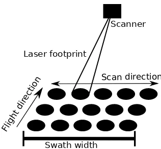
Figure 2.1Conceptualization of airborne lidar scanning. Scan direction (scan line) is typically perpendicu-lar to the flight direction. The area covered during scanning while an aircraft flies in a constant direction is called the swath.
Airborne lidar point clouds
Airborne lidar data acquisition and resulting variability of point density depend on a flight plan (flight mission), scanner, movement of the aircraft (platform), georectification using Global Navigation Satellite System (GNSS) such as Global Positioning System (GPS) and Inertial Navigation System (INS) with Inertial Measurement Unit (IMU), and environmental conditions[Lemmens, 2011; Wehr & Lohr, 1999].
In an idealized case, aircraft flies at a constant speed, direction, and altitude above ground level with zero roll, pitch, and yaw and known position. A line scanner aboard the aircraft scans the mapped area in the direction perpendicular to the line of flight. This scanner would ideally capture a complete scan line at once with constant spacing between the points on the ground. Furthermore, the speed of the aircraft would be such that the point spacing in the scan line is the same as the spacing between the scan lines. Finally, the aircraft would fly in straight parallel lines separated by the width of the scan line (swath) so that the individual swaths have minimal overlap and, at the same time, cover the entire surveyed area. Part of this concept is captured in Fig. 2.1. For a flat terrain without vegetation or other objects, the result would be a regular grid of points. However, none of these idealized procedures are actually fulfilled in real world conditions. Since the point clouds can still be well understood using this idealized state, point clouds were described asmisbehaved rasters[Lutz, 2011]. In the following paragraphs we describe density anomalies and related errors common for airborne lidar.
Point pattern
(a) (b) (c) (d)
Figure 2.2Scan patterns for basic types of sensors[Fernandez-Diaz et al., 2014; Kim et al., 2013; Wehr & Lohr, 1999]: (a) oscillating mirror (e.g., EAARL), (b) fiber scanner (e.g., TopoSys system), (c) rotating polygon, (d) elliptical scan pattern (e.g., Palmer scanner).
Figure 2.3Point cloud from several overlapping swaths with elliptical scan patterns. Elliptical scanning causes higher density of points at the edge of each swath. Data source: NOAA/NASA/USGS[1999].
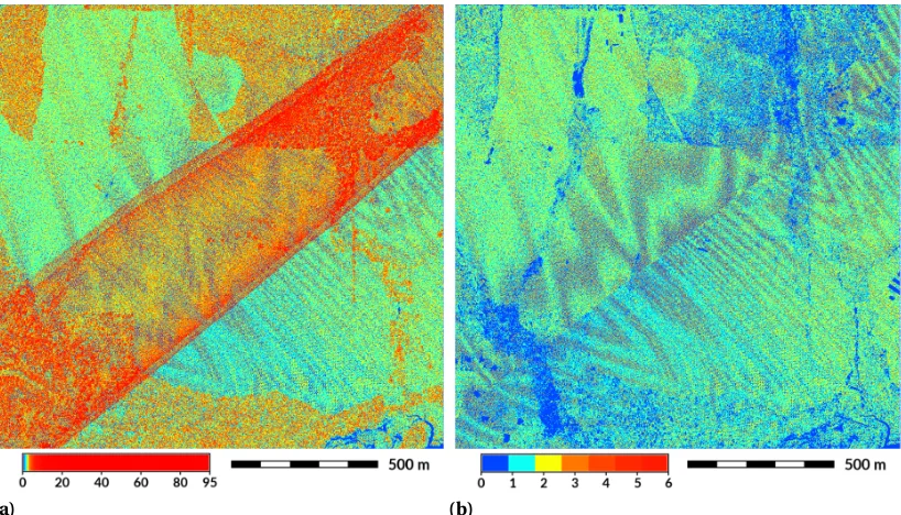
(a) (b)
Figure 2.4Density of points increases towards the end of the scan line (a) and peaks at the very end (b). Extent of figure (b) is highlighted in figure (a). Only points with specific source ID, scan direction, and user data field are displayed. Data source: NC Floodplain Mapping Program[2015].
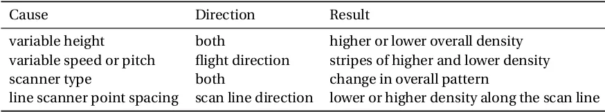
Table 2.1Sources of point density anomalies in the flight direction and the direction perpendicular to the flight direction (typical scan line direction for line scanners).
Cause Direction Result
variable height both higher or lower overall density
variable speed or pitch flight direction stripes of higher and lower density
scanner type both change in overall pattern
line scanner point spacing scan line direction lower or higher density along the scan line
Scan line anomalies
(a) (b)
Figure 2.5Changing speed of the aircraft or changes of its pitch will result in areas with higher and lower point density along the flight line (here approximately north-south direction). Darker areas indicate lower density of points while lighter areas indicate high density. Number of points at 6 m resolution (a) and 5 m resolution (b). Data source: NCALM[2009](a), NOAA[2008](b).
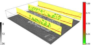
Figure 2.6Example of interactive exploration of density banding using profile (transect) of density (red), el-evation (light blue) and exaggerated elel-evation map (dark blue). To see potential elel-evation banding (waves), we created the profile along a road which does not contain abrupt changes in elevation, thus potentially revealing banding. This dataset does not show signs of elevation banding. Data source: NOAA[2008].
Banding
the flight line,[Toth, 2009]. See Fig. 2.5 for an example of these stripes. This effect is calledbanding
[Carter, 2005]. To mediate this effect, helicopters may be used to obtain high-resolution coverage with more uniform distribution of points because they can easily control their speed[Lemmens, 2011].
Another cause of banding is a change in pitch of the airplane. In this case, the result is again irregular point density and possibly also errors in measured elevation[Carter, 2005]. When the aircraft changes its pitch due to environmental conditions or human error and at the same time there is an error in the recorded pitch value, the measured distance to the point is associated with an incorrect position. The result of elevation errors is artificially undulating terrain. Whether the banding is just in density or in elevation as well can be examined by comparison to another DEM or by creating a profile of the point density and the DEM (Fig. 2.6).
Aircraft altitude variations
Point density is also influenced by the height of the aircraft above ground. Lower height above ground will cause smaller point spacing in the scan line and vice versa. Variable height during the flight will thus result in variable density. A height that is too low may even cause the swath to be too narrow to overlap or at least touch the adjacent swath. For some scanners, such as those with an elliptical scan pattern, changes in height also influence spacing in the flight direction.
In mountainous areas, the changes of terrain elevation together with the constant altitude (height above sea level) of the aircraft cause variable densities in the higher and lower situated areas when the sensor is not adjusted. Similarly, high slopes result in less points capturing the surface. Although the horizontal density stays the same in this case, there will be less points covering a given surface in a sloped area in comparison to a flat area.
Table 2.2Density changes related to changes in swath overlaps.
Cause Swath overlap change Result
height (uncorrected) smaller or no overlap possibly gaps
roll (uncorrected) smaller or no overlap possibly gaps
human or navigation error missing or additional swath gaps or higher density
Swath overlaps
Figure 2.7Example of a complex point distribution. The area is completely covered by one swath and partially covered by another. The border of the second one reveals the doubled scan pattern and higher density at the end of the scan line. There are bands of higher and lower densities in the direction of the flight. Other density variations are related to vegetation and the small area with missing points on the left is caused by water body. Data source: Wake County[2013].
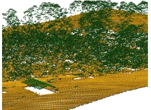
Figure 2.8Corduroy effect visible on the interpolated digital surface model visualized in 3D (a) and a derived skyview factor visualization[Zakšek et al., 2011]overlayed with the source point cloud (b). Data source: NASA/USGS[2003].
collecting the swaths with overlaps is related to mitigating errors introduced by the acquisition of the position and orientation of the aircraft, which are used to derive point coordinates. Collecting swaths with overlap generates redundant information which can be used to align individual swaths by eliminating the horizontal and vertical time-dependent shifts[Lemmens, 1997]. These shifts, occurring due to systematic GNSS/GPS and INS/IMU errors, can then be minimized, for example, by least squares matching[Toth, 2009].
(a) (b)
Figure 2.9(a) Swath overlap as the main source of variation in point density. (b) Moire effect in the density pattern visible in the classified ground points. Abrupt change in the pattern which follows a straight line marks the transition between swaths and removed swath overlap. Figures show the number of points at 1 m resolution. Data source: Wake County[2013].
(a) (b)
the point density patterns arises. When combined with errors in positioning, this leads to an abrupt change in point elevations[Shrestha et al., 2007]. When the variable point density at the swath overlap is not addressed, it may be an issue for vegetation-related metrics. However, for terrain reconstruction, it usually poses a problem only when the elevation of the swaths is not correct (Fig. 2.10). Furthermore, the size of swath overlaps may vary due to changes in aircraft height above ground, due to aircraft’s roll, or due to human and navigation errors, (Tab. 2.2). Modern systems often try to account for changes in height by adjusting the scan line and try to reduce these errors using on-board checks.
Moire and corduroy effects
Overlapping point patterns from two overlapping swaths or generally from two scan patterns often lead to a moire effect in the point density pattern (Fig. 2.9). Additionally, when two alternating series of scan lines overlap as a result of swath overlap, scanning back and forth with a line scanner, or doubled scan pattern and, at the same time, points in these series are not correctly georeferenced, the digital elevation model will contain stripes of higher and lower elevation resulting in a corduroy effect (Fig. 2.8).
(a) (b)
Figure 2.11Areas without points caused by water bodies (a), dark asphalt roof (b). Data source: Wake County[2013].
Surface material properties and obstructions
the pulses. Depending on the wavelength used by the lidar sensor, some surfaces, mainly water and dark asphalt, return a weaker signal or do not return any pulses, which results in lower point return intensities or no recorded points at all. Lower intensities may thus be an indicator of lower densities and vice versa. The surfaces which are most likely to suffer from these issues are water bodies, wetlands, and some types of roads and roofs (Fig. 2.11).
(a) (b)
(c) (d)
Figure 2.12Differences in point distributions and patterns between first return points (a, c) and classified bare ground points (b, d). Figure (a) shows first return points and (b) ground points. Figures (c) and (d) show point density as a number of points per 3 feet (1 meter) cell. Data source: NC Floodplain Mapping Program[2015].
Vegetation and horizontal point density
(a) (b)
Figure 2.13Horizontal point pattern in vegetated and non-vegetated areas: (a) All return points have a reg-ular pattern in open areas combined with irregreg-ular distributions in the vegetated areas. (b) Ground points in areas without vegetation have the original pattern, while in the areas with vegetation the distribution is much sparser. Data source: NC Floodplain Mapping Program[2015].
(a)
(b)
Figure 2.14Vertical distribution of lidar points in natural forest (left) and a planted forest (right) in a 220 m long and 30 m wide transect of a forested area (a). Skewness of point elevations along the same transect without ground points (b). Data source: NC Floodplain Mapping Program[2015].
Point density in the vertical direction
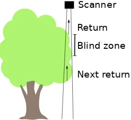
Scanner
Blind zone Return
Next return
Figure 2.15The blind zone effect, i.e., no points recorded after a given record, may cause the omission of points in certain parts of the vegetation or on the ground.
is registered, may cause gaps in the vertical point distribution[Shrestha et al., 2007]. For example, lidar sensor Leica Geosystems,[2016]reports a blind zone distance of 2.8 m.
Table 2.3Errors in elevation, their relations to density, and their causes
Cause Result in density Result in elevation
occlusion, low reflectivity gaps smooth areas
pitch changes and recording errors dense stripes terrain banding vertically unaligned swaths or scan lines abrupt changes corduroy effect
Distribution of ground points
Ground points usually have much higher variability in density (Fig. 2.12) and pattern (Fig. 2.13). For highly dense vegetation, pulses don’t penetrate all the way to the ground[Lemmens, 1997]causing gaps in the ground point distribution (Fig. 2.12). Even if the pulses penetrate to the ground, the density of points is much lower than in non-vegetated areas (Fig. 2.13).
(a) (b)
Figure 2.16Lower density of ground points in vegetated areas or lack of points in wet areas usually causes these areas to be smoother than the rest of the area when points are interpolated into a DEM: (a) Lower density of all return points around a stream and in a vegetated, supposedly wet area (marked in blue). (b) Classified ground points (red) missing in some areas completely. The influence on the DEM becomes most apparent when the DEM is used to derive additional products such as the shaded relief here. Data source: NC Floodplain Mapping Program[2015].
SfM-derived point clouds
Numerous low cost surveys are now performed thanks to the availability of small unmanned aircraft systems (sUAS). Although lidar or other sensors can be mounted on small UASs[Yang & Chen, 2015], for cost and carrying capacity (payload) reasons, in most cases only standard RGB consumer cameras are currently being used. The advantage of small UASs surveys in comparison to airborne lidar surveys is the collection frequency, i.e., the high temporal resolution, which can be achieved [Mathews & Jensen, 2013]thanks to the availability of the UAS platforms and the time efficiency of surveys.
The images taken by the camera can be processed by various computer vision and photogram-metric techniques. The most common technique today is the Structure from Motion pipeline (SfM). Compared to lidar where the individual points in the point cloud result from the direct measurement of the sensor, SfM is a set of algorithms which use well defined features captured in multiple images to generate point clouds[Wallace et al., 2016]. We refer to a point cloud created in this way as an SfM-derived point cloud.
densified in the next step[Furukawa & Ponce, 2010; Lucieer et al., 2011]. The resulting dense point cloud is typically more dense than the current airborne lidar point clouds. Sources of variability of point densities are summarized in Table 2.4.
Color information (RGB)
Since the SfM-derived point cloud is usually a result of processing RGB images, RGB information is associated with an individual point. This is different from lidar scanners which have an intensity (of a return) associated with each point, although some lidar scanners (e.g., FARO) can associate RGB values with individual points. Unlike the intensity associated with lidar points, RGB values have a clear interpretation. It can be used in many applications reducing the need for fusion with other data sources or calibration which would be the case for lidar intensity. RGB values (spectral information) are used for further analysis, resulting in a detailed representation, e.g., of the upper canopy[Dandois & Ellis, 2013].
Table 2.4Variable point density sources for SfM-derived point clouds
Source Result Possible solution
low/no vegetation penetration missing ground points fly in leaf-off conditions
occlusion by other objects gaps add more nadir or oblique images
shadows missing/incorrect points fly at different time/weather
snow cover missing/incorrect points use NIR
Point pattern
The SfM-derived point clouds will have typically higher density than point clouds from aerial lidar surveys[Wallace et al., 2016]because small scale, detailed studies benefit the most from the usage of UASs. With hundreds and even thousands of points per square meter, the SfM algorithm and the subsequent dense point cloud processing often require high computational power and long processing times[Wallace et al., 2016].
(a) (b)
Figure 2.17Density pattern from SfM-derived point cloud with moire effect. Figures show the number of points at 0.5 m resolution. Data source: Jeziorska et al.[2016].
context of DEM processing, can be used similarly for SfM-derived point clouds.
Platform stability and altitude variations
Point densities are directly related to ground sampling distance (GSD), which is given by flight altitude and camera resolution. To enable a homogeneous resolution of the reconstructed surface and orthophoto, GSD should be kept constant. In mountainous landscapes the elevation differences within a single image can reach several hundred meters. In these cases, tilting the camera from the nadir angle may be beneficial[Bühler et al., 2017]. In the case of light-weight UAS platforms, the camera can often get tilted unintentionally due to strong winds. Large rotation angle can then potentially lead to poor image ground resolution, insufficient overlap, and overall low accuracy of results[Yang et al., 2016].
Material properties, shadows
as demonstrated in Fig. 2.18.
(a) (b) (c)
Figure 2.18Elevation difference in meters between two UAS surveys collected 1 hour apart (a) caused by the change in cast shadows (b, c). Teal area is shadowed in (b) but not in (c). Data source: Jeziorska et al.
[2016].
Vegetation, horizontal and vertical point distribution
Figure 2.19140 m long and 5 m wide vertical slice (transect) of a point cloud obtained from lidar and an SfM-derived point cloud. Data source: Jeziorska et al.[2016](SfM), NC Floodplain Mapping Program[2015] (lidar).
does not capture the internal tree structure and can even omit a tree. It has been demonstrated that very high forward overlap of captured images is correlated with high point densities resulting in enhanced vegetation reconstruction[Dandois et al., 2015; Torres-Sánchez et al., 2018]. Due to the required forward and side image overlap, the same tree is captured many times on multiple images. Since SfM reconstruction assumes the image features are not moving, increased wind speed that sways the tree branches may decrease point cloud density due to lack of consistency[Torres-Sánchez et al., 2018]. This doesn’t happen with airborne lidar because each point is captured at only one given moment.
Ground points and digital terrain model (DTM)
Further issues come when considering usage of SfM-derived point clouds for creating DTM. SfM requires each place to be visible from multiple locations which means that each place on the ground needs to be captured in multiple images. This is usually not fulfilled[Wallace et al., 2016]and a DTM from different source needs to be used to supplement the SfM-derived point cloud, especially for precise measurements and in forested areas[Dandois & Ellis, 2013]. However, compared to terrestrial lidar, SfM-derived point clouds can provide a better representation of terrain in areas without high vegetation, although even low vegetation causes bias in the elevation values[Gruszczy ´nski et al., 2017].
Decimation and homogenization of point clouds
Decimation (thinning) is the reduction of the number of points in a point cloud while preserving selected properties of the point cloud. Decimationis a relatively new preprocessing step that has resulted from improved sensor design, system processing, and the general notion that more data are always better regardless of the terrain or subsequent application[Zhao et al., 2016].
Considering the hard-to-avoid causes of point density variations, algorithms working with lidar point clouds need to account for these variable point densities[Brodu & Lague, 2012; Tarsha-Kurdi et al., 2007]. However, for digital elevation models, making the density more uniform is often sufficient and the most efficient solution[Anderson et al., 2006].
Elevation surface modeling
The original and most common use of lidar data, especially aerial lidar data, is the creation of digital elevation models (DEMs), specifically digital terrain models (DTMs) capturing only ground surface as opposed to including trees and buildings. The desired density of point clouds for creating ground surface depends on the desired resolution of the surface. However, even high-precision DTMs generally don’t need to use the full density of the current point cloud datasets[Duldulao, 2009; Jia et al., 2013; Petras et al., 2016; Puetz et al., 2009; Singh et al., 2015; Zhao et al., 2016]. Decimation is advantageous for deriving DTMs from different types of datasets including airborne, terrestrial lidar, and SfM-derived point clouds. In the case of airborne lidar, decimation can normalize the density anomalies resulting from swath overlaps. For terrestrial lidar, the density around the station is very high and decreases significantly further from the station. Therefore, there are a lot of points right around the station which are not needed for creating a DTM and can be safely removed from the dataset. In general, if all the redundant points are left in the dataset (not decimated), it doesn’t negatively influence the result. However, they may increase the processing time significantly[Liu et al., 2007]which is an important consideration and a reason to remove them. On the other hand, high point density is needed to classify and distinguish ground surface points from points which represent returns from trees, buildings, and other objects[Anderson, 2008; Huang et al., 2011; Huising & Gomes Pereira, 1998]as well as to preserve sharp edges of the objects such as building roofs.
Classification of point clouds
Automatic classification of point clouds includes methods for separating ground and non-ground points such as progressive morphological filter[Zhang et al., 2003], surface curvature or edge-based algorithms[Brovelli et al., 2004; Hu et al., 2014], or the multiscale curvature classification[Evans & Hudak, 2007]. Classification also includes classifying points into classes such as buildings or high vegetation. These classifications often involve performing segmentation, using the intensity of pulse return associated with each point, and fusing the data with other data such as imagery. As mentioned earlier, high density is usually an advantage for classification, but decimation may be a part of certain classification process, such as identifying a flat roof segment.
3D object reconstruction and 3D metrics
Some methods use voxelization of space which typically reduces the number of points or replaces groups of points by 3D cubes (depending on the implementation). This technique was used to characterize forest canopy fuel properties[García et al., 2011], internal patterns of vegetation[Petras et al., 2017b], fine-scale bird habitat[Sasaki et al., 2016], and detailed tree models[Brolly et al., 2013; Gorte & Winterhalder, 2004]. These methods can often use relative point counts based on absolute point counts in the neighborhood[Kumar et al., 2015; Petras et al., 2016], thus potentially reducing the influence of variable point density in the point cloud.
For many forest and tree related metrics, non-uniform point density is usually not an issue[ Hop-kinson et al., 2004; Mehtätalo et al., 2014]. This includes determination or estimates of stem location, tree height, basal area, height to first branch, stem density, timber volume, crown base height, and stem diameter (DBH, diameter at breast height). For example, stem position and diameter may be determined by fitting a cylinder on the points using Hough transformation[Simonse et al., 2003]. In this case, the position of the points on the cylinder matters, but it doesn’t matter if the points are uniformly distributed around it. However, a low point density can decrease the accuracy of all tree level predictions[Dalponte et al., 2009].
Decimation techniques
Decimation techniques range from simple ones, such as random sampling, to complex decimations based on shape of the objects described by the point cloud. Random sampling can be based on the ordinal number of a point within the point cloud (count-based sampling). This sampling highly depends on the ordering of the points within the point cloud (data file) and may not give expected result when the points are in some special order. However, this technique works well for terrestrial and airborne lidar point clouds when points are ordered by collection time[Pirotti & Tarolli, 2010] and used for creation of DTMs[Petras et al., 2016]. True random sampling is based on comparing a (pseudo) random number with a threshold which requires more computational time because a random number needs to be generated for each point.
Conclusion
We provided an overview of different issues in point clouds focusing on density anomalies and related errors. Based on our findings, we strongly suggest that a thorough examination of the spatial distribution of point density is conducted at the start of any analysis which is using point clouds. This should be done in parallel with comparison to expected point cloud properties based on the scanner type and collection method. Knowing the role of the point cloud and its density in the analysis is crucial and we showed several cases when point density variations may indicate errors in point positions. Special care should be given to point clouds used for analysis which is highly influenced by the point cloud density, such as many vegetation-related metrics. We also suggest that a description of such examinations is always included in scientific publications and technical reports and we call for more research of methods which account for or remove density anomalies.
Acknowledgements
The airborne lidar data include NC Quality Level 2 lidar (NC QL2) collected by North Carolina Floodplain Mapping Program in 2015[NC Floodplain Mapping Program, 2015]and North Carolina Wake county lidar collected in 2013[Wake County, 2013]. Further, we use the Nantahala dataset from the National Center for Airborne Laser Mapping[NCALM, 2009]and coastal lidar data from the pre-hurricane Isabel survey in 2003 collected with the National Aeronautics and Space Administration (NASA)/U.S. Geological Survey (USGS) Experimental Advanced Airborne Research Lidar (EAARL) [Bonisteel et al., 2009]. The phodar point cloud is based on imagery from a 2016 UAS flight processed by Agisoft PhotoScan[Jeziorska et al., 2016].
CHAPTER
3
Homogenization and decimation of point clouds
Reprint
Vaclav Petras, Anna Petrasova, Justyna Jeziorska, and Helena Mitasova. 2016. Processing UAV and lidar point clouds in GRASS GIS. In:ISPRS-International Archives of the Photogrammetry, Remote Sensing and Spatial Information Sciences, XLI-B7, pp. 945–952. DOI 10.5194/ isprsarchives-XLI-B7-945-2016
Attribution
I developed the methods, case studies, processed data, and prepared the manuscript. Anna Pe-trasova and Justyna Jeziorska processed the UAV and low-cost indoor scanner data. Helena Mitasova provided critical revisions to the manuscript.
Published software
I have extended and refactored the underlying binning code ofr.in.lidarGRASS GIS1module. Further, I created a newv.decimate module which decimates using grid-based decimation. The module can also decimate just based on count and since it preserves the original points, so it can be used for sampling. I also added several filtering and count-based decimation functions tov.in.lidar module. I developed a newr3.in.lidar module for binning in 3D andr.local.relief module for computing local relief model which I used for the analysis of the decimated point clouds.
Educational material and provided training
I led a 4-hour hands-on workshop at the Center for Geographic Analysis, Harvard University during FOSS4G 2017 in Boston and also a 2-hour geospatial studio at North Carolina State University, Center for Geospatial Analytics. The workshop title wasProcessing lidar and UAV point clouds in GRASS GISand I demonstrated how to process and understand a point cloud with uneven point densities using both tools which were already in GRASS GIS and tools which I added. Teaching material for this workshop is available online2and was translated to Spanish3by the GRASS GIS community. A short version of this material is included in the Appendix B.
2https://grasswiki.osgeo.org/wiki/Processing_lidar_and_UAV_point_clouds_in_GRASS_GIS_
(workshop_at_FOSS4G_Boston_2017)
3https://grasswiki.osgeo.org/wiki/Processing_lidar_and_UAV_point_clouds_in_GRASS_GIS_
PROCESSING UAV AND LIDAR POINT CLOUDS IN GRASS GIS
V. Petrasa∗, A. Petrasovaa, J. Jeziorskaa,bH. Mitasovaa,
aDepartment of Marine, Earth, and Atmospheric Sciences, North Carolina State University - (vpetras, akratoc, hmitaso @ncsu.edu) bDepartment of Geoinformatics and Cartography, University of Wroclaw - ([email protected])
Commission VII, SpS10 - FOSS4G: FOSS4G Session (coorganized with OSGeo) KEY WORDS:3D rasters, decimation, sampling, binning, LAS, PDAL, PCL, Kinect
ABSTRACT:
Today’s methods of acquiring Earth surface data, namely lidar and unmanned aerial vehicle (UAV) imagery, non-selectively collect or generate large amounts of points. Point clouds from different sources vary in their properties such as number of returns, density, or quality. We present a set of tools with applications for different types of points clouds obtained by a lidar scanner, structure from motion technique (SfM), and a low-cost 3D scanner. To take advantage of the vertical structure of multiple return lidar point clouds, we demonstrate tools to process them using 3D raster techniques which allow, for example, the development of custom vegetation classi-fication methods. Dense point clouds obtained from UAV imagery, often containing redundant points, can be decimated using various techniques before further processing. We implemented and compared several decimation techniques in regard to their performance and the final digital surface model (DSM). Finally, we will describe the processing of a point cloud from a low-cost 3D scanner, namely Microsoft Kinect, and its application for interaction with physical models. All the presented tools are open source and integrated in GRASS GIS, a multi-purpose open source GIS with remote sensing capabilities. The tools integrate with other open source projects, specifically Point Data Abstraction Library (PDAL), Point Cloud Library (PCL), and OpenKinect libfreenect2 library to benefit from the open source point cloud ecosystem. The implementation in GRASS GIS ensures long term maintenance and reproducibility by the scientific community but also by the original authors themselves.
1. INTRODUCTION
Current methods of acquiring data to represent terrain or surface are often associated with large number of points in unordered point clouds. These points are collected non-selectively in case of lidar devices or generated during imagery processing as in the case of imagery collected by unmanned aerial vehicles (UAV). Not all of these points are necessarily important for creating a digital elevation model (DEM) of a given area (Brasington et al., 2012). Thus omitting the unnecessary points is desired since it is computationally challenging to process the acquired point clouds (Rychkov et al., 2012). Even with increasing hardware power, we are collecting larger points clouds which are more challenging to process.
There are two basic approaches for processing large number of points. The first approach is binning which creates a raster from a point cloud. Binning is a powerful analytical method which can be extended into 3D space in order to reveal vertical structure of vegetation (Gorte and Winterhalder, 2004). The second approach is decimation, also referred to as thinning or sampling, which re-duces number of points of a point cloud. In this research, we are testing two decimation techniques, count-based decimation (Pirotti and Tarolli, 2010) and grid-based decimation, to see how they perform when applied to different types of data. Our ob-jective is to determine how many points we can remove from a point cloud and still preserve enough details in the digital ele-vation model. Additionally, we compare the performance of the two techniques to evaluate whether there is a need for both tech-niques.
Geospatial methods can be implemented either as standalone tools or integrated into a larger software package. We want the im-plementation of our methods to be accessible in the long-term,
∗Corresponding author
and available for further review and improvement. Furthermore, the methods should be easily used with other geospatial process-ing tools. For these reasons, we use GRASS GIS (Neteler et al., 2012), a free, libre and open source geospatial information system, for our geospatial processing. We also implemented the methods presented in this paper, namely count-based decimation, grid-based decimation and three dimensional binning, in GRASS GIS.
2. DATA
For this study we are using four different point cloud types: air-borne lidar and ground-based lidar point clouds, points from a low-cost indoor scanner (the Microsoft Kinect), and a point cloud derived from data obtained from UAV imagery using structure from motion (SfM) technique. Our study site is a rural area south of Raleigh, North Carolina, USA. The data for our study area, the Sediment and Erosion Control Research and Education Fa-cility (SECREF) at the Lake Wheeler Road Field Laboratory of North Carolina State University, were collected in 2013 by Wake county with airborne lidar. The point cloud was classified by the data provider. We used only points classified as ground (class 2) for our study. The ground-based lidar measurements were done in 2009 on a small part of the SECREF site (Starek et al., 2011) using Leica Geosystems ScanStation 2. The measurement was done from two sites and the point clouds were merged together. The data obtained by the Kinect scanner capture a scaled physical model molded from sand. The 0.37 m×0.35 m mold was de-rived from the airborne lidar data for the SECREF site. The data generated by SfM from UAV imagery are from a location west of the SECREF site and not from the SECREF site itself due to the limits on where the UAV could be flown (Jeziorska et al., 2016).
To understand the spatial distribution of points in the point cloud we look at the number of points per raster cell. Figure 1 shows
The International Archives of the Photogrammetry, Remote Sensing and Spatial Information Sciences, Volume XLI-B7, 2016 XXIII ISPRS Congress, 12–19 July 2016, Prague, Czech Republic
This contribution has been peer-reviewed.
Figure 1: The number of points per cell for point cloud obtained using airborne lidar (raster resolution 1.5 m)
Figure 2: The number of points per cell for point cloud obtained using UAV imagery (raster resolution 0.5 m)
uniform distribution of the points classified as ground in the air-borne lidar dataset. The only non-uniformities we can see are caused by presence of buildings (places without any points), veg-etation (places with lower point density) and the scanning
pat-Figure 3: The number of points per cell for point cloud obtained using ground-based lidar (raster resolution 0.5 m). Note that the color table uses red color for values from 80 up to the maximum
which is 18 thousand points per cell.
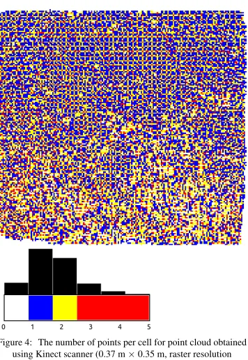
Figure 4: The number of points per cell for point cloud obtained using Kinect scanner (0.37 m×0.35 m, raster resolution
0.002 m)
tern (lines of slightly higher and lower density). Figure 2 shows the spatially variable number of points per cell for the the UAV dataset which is primarily caused by the variable vegetation cover (areas with and without crops) and by artifacts from the SfM pro-cessing step. Figure 3 shows the number of points per cell for the ground-based lidar measurement. The highest density of points is in 10 m radius around the ground-based lidar stations. Figure 4 reveals the regular, grid pattern of the point cloud acquired by the Kinect scanner.
3. APPROACH
In this section, we first reiterate why we choose an open source implementation in GRASS GIS. We follow with an overview of how point clouds are processed in GRASS GIS highlighting newly implemented 3D binning and integration with other open source projects. Then, we explain the binning process in detail
The International Archives of the Photogrammetry, Remote Sensing and Spatial Information Sciences, Volume XLI-B7, 2016 XXIII ISPRS Congress, 12–19 July 2016, Prague, Czech Republic
This contribution has been peer-reviewed.
which is also important as a base for the grid-based decimation technique. Further, we discuss both newly implemented tech-niques for decimating point clouds, namely count-based decima-tion and grid-based decimadecima-tion. Finally, we discuss our approach for comparing decimated point clouds.
3.1 Open source implementation
We want to assure that the newly developed methods and other methods used in this study can be reviewed. To review a method’s implementation, its source code must be publicly accessible. In order to build or improve upon the source code, the code should be available under an open source1 license. Furthermore, we
want to ensure that all methods we are using and developing will remain accessible in the long term. GRASS GIS has long his-tory of preserving algorithms over several decades (Chemin et al., 2015) with changes and updates to reflect new hardware, plat-forms, types of data and user needs. The implementation of the methods in GRASS GIS ensures long-term accessibility thanks to an active community which has now worked on GRASS GIS for more than 30 years. We can also see a wide variety of tools being constantly2added. In order to build complex analytic workflows,
we can take advantage of the wide range of geospatial tools of-fered by GRASS GIS such as remote sensing (Neteler and Mi-tasova, 2008) or spatio-temporal data processing tools (Gebbert and Pebesma, 2014), and use them together with our newly de-veloped methods.
3.2 Processing point clouds in GRASS GIS
The first step in the typical point cloud processing workflow in GRASS GIS is to explore the point cloud by counting the number of points per raster cell usingr.in.lidarmodule3with different
resolutions. We determine the spatial distribution and density of points of different classes and the optimal resolution for further analysis.
Further processing typically consists of computing digital ele-vation model, height above surface, and several other statistics based on point count, height of points, and intensity of points. This functionality is available inr.in.lidarmodule for 2D rasters and inr3.in.lidarfor 3D rasters. Both 2D and 3D rasters can be further processed by corresponding processing tools. The 3D raster can also be decomposed into series of 2D rasters to take advantage of the standard tools for image processing and classi-fication available in GRASS GIS.
To create a smooth surface based on a point cloud, we can import the points to GRASS GIS usingv.in.lidarmodule which creates vector points. These points can be later interpolated to create a smooth surface typically representing digital elevation model. Several interpolation methods are available for example, inverse distance weighting implemented inv.surf.idwmodule, bicubic and bilinear spline interpolation with Tykhonov regularization (Brovelli et al., 2002) both implemented inv.surf.bspline mod-ule, and regularized spline with tension technique (Mitasova et al., 2005) implemented inv.surf.rstmodule. The aforementioned lidar modules can limit the import through a number of parame-ters including spatial extent, area, and return number or class if these are available.
1We understand open source as defined by the Open Source Initiative
atopensource.org/osd.
2At the time of writing last added GRASS GIS add-on module called r.randomforestwas added less than a week ago.
3The individual programs, tools, plug-ins, and functions in GRASS
GIS are called modules.
Figure 5: Point cloud obtained using airborne lidar in a small selected area with a patch of trees in the middle and a building (same as in Figure 6). Points classified as ground by progressive
morphological filtering from PDAL are in yellow; all the other points are in green.
Besides GRASS GIS functionality we can take advantage of meth-ods and tools implemented in other open source packages. We present a prototype ofv.in.pdalmodule which integrates several features from the Point Data Abstraction Library (PDAL) includ-ing progressive morphological filter for ground point classifica-tion (Zhang et al., 2003) from the Point Cloud Library (PCL). This method can be used as an alternative to the multiscale cur-vature classification algorithm (Evans and Hudak, 2007), imple-mented inv.lidar.mccadd-on4module, and the edge-based
li-dar data filtering method (Brovelli et al., 2004), implemented in
v.lidar.edgedetection,v.lidar.growing, andv.lidar.correction mod-ules in GRASS GIS. An example result from the progressive mor-phological filter is in Figure 5.
For reading data from the low-cost indoor scanner, Microsoft Kinect, we use a module calledr.in.kinectwhich uses OpenK-inect libfreenect2 library (Xiang et al., 2016) to communicate with the device. This module is used in Tangible Landscape sys-tem which is a collaborative modeling environment for analysis of terrain changes coupling a scanner, projector and a physical 3D model with GRASS GIS (Petrasova et al., 2015).
3.3 Binning
Binning is the conversion of points into a regular grid. The bin-ning of points with X and Y coordinates starts with the overlay of a grid of bins over the points. A bin can be a rectangle, hexagon or generally any shape which can create continuous grid. When creating a raster from a point cloud, the bin is a raster cell which is square or rectangular. The value associated with a bin is the count of points falling into the given bin (Lewin-Koh, 2011). The analogous concept in univariate statistics (one dimension – 1D) is a histogram, so the result of this binning can be called 2D (two dimensional) histogram. We use binning to count the number of points per raster cell to see the density of points.
The concept of binning can be extended when the points have an-other value associated with them. For lidar data this value can be the Z coordinate or intensity. The value for a bin is computed as univariate statistics from the values of all points in the bin. For example, computing the mean value of Z coordinates yields a raster representing the digital elevation model. Another exam-ple is the range of Z coordinates which can be used as a rough estimate of vegetation height.
4Add-on modules are not part of the standard installation of GRASS
GIS but can be installed separately using theg.extensionmodule. The International Archives of the Photogrammetry, Remote Sensing and Spatial Information Sciences, Volume XLI-B7, 2016
XXIII ISPRS Congress, 12–19 July 2016, Prague, Czech Republic
This contribution has been peer-reviewed.
Figure 6: The result of 3D binning a point cloud obtained using airborne lidar (using all classes) in a small selected area with a
patch of trees in the middle. The visualization shows slices of the resulting 3D raster. The variable visualized in yellow, green,
and red is the proportional count of points per vertical column where yellow means 0% of points from a vertical column are in
the given 3D cell (voxel) and red means that more than 40% of points from a given vertical column are in the given 3D cell. The horizontal plane is colored in gray scale according to the number of points per 2D cell which is a result of 2D binning at 2 m
resolution.
Binning into a 3D (three dimensional) grid of cubes (rectangular cuboids) creates a 3D raster. Same statistics can be computed as in the case of 2D raster but not from the Z coordinate as it is used to determine position in the 3D grid in the same way as X and Y coordinates are used. By dividing bin values in each vertical column by value of a corresponding bin from a 2D binning result, we obtain the proportional (relative) value of a given variable that is not influenced by relative point density. The example result for the selected section of the airborne lidar dataset is shown in Figure 6 which represents vegetation structure as vertical slices of a 3D raster.
3.4 Count-based decimation
Count-based decimation is the removal (or preservation) of ev-eryn-th point based on its ordinal number in the set of points. Depending on the dataset structure and selectedn, such point se-lection may be biased and does not ensure spatialy homogenious decimation. The advantage of this method is, however, its sim-plicity resulting in very fast point processing.
Specifying valuerto “remove every n-th point” or valuekto “keep every n-th point” is reasonably straighforward. For exam-ple, it is clear that removing every third point results in removal of one third of points. However, when we need to preserve a given percentagepof points, specifying the right valuesrandk
gets more complicated, because we can remove only certain frac-tions of points. Some percentage values can be easily converted torandkvalues as visible in the Table 1. For a specific per-centagepof points the following equations can be used to obtain approximate values ofrandk. Forp >= 0.5the valueris:
r=
1 1−p+ 0.5
(1)
wherebacis the whole part ofaobtained by trimming the deci-mal part of the numbera.
Forp <0.5the valuekis:
k=
1
p+ 0.5
(2)
p r
16.6% 6
20.0% 5
25.0% 4
33.3% 3
50.0% 2
p k
66.6% 3
75.0% 4
80.0% 5
83.3% 6
90.0% 10
Table 1: Values ofrandkfor selected fractions of removed pointspin percent
3.5 Grid-based decimation
2D grid-based decimation of points creates a subset of spatially uniformly distributed points with representative heights. This subset of points can later be used to interpolate smooth digital terrain model and topographic parameters. When binning vector points to raster, Z coordinates of points in a grid cell are counted, summed, averaged or processed in other ways. To perform the grid-based decimation, we average the X and Y coordinates of all the points in the given grid cell to get a position of a new point. Average is defined as a sum of all values divided by the number of values. However, considering the often large numbers repre-senting horizontal coordinates, summing all the X or Y coordi-nates of all points in a grid cell could result in truncating the sum and loosing precision. For this reason, we use cumulative mov-ing mean5which requires us to store only one value rescaled by
the number of values we processed up to that point. Cumulative moving meancini-th step is defined as:
ci=ci−1+
xi−ci−1
i (3)
whereciis cumulative mean in the current step,ci−1is
cumula-tive mean in the previous step,xiis the current value andiis the
current step number.
3.6 Comparing decimated point clouds
To compare the two newly implemented decimation techniques, we decimated the given point cloud using count-based decima-tion and grid-based decimadecima-tion with different settings influenc-ing the number of preserved points. We interpolated a surface from each decimated point cloud using regularized spline with tension technique (Mitasova et al., 2005) as implemented in the
v.surf.rstmodule. We are interested in how the distinct terrain features are preserved when lower number of points is used. To identify these features we use local relief model (LRM) extraction algorithm (Hesse, 2010), implemented in ther.local.reliefadd-on module which identifies terrain features based on their difference to terrain trend. The example of LRM enhancing digital elevation model visualization is shown in Figure 7.
We decimated each point cloud using the count-based method several times while changing number of removed points from less progressive removal to more progressive removal. Similarly, we decimated the point clouds using the grid-based method with coarser resolution each step. After interpolating and computing the local relief models, we correlated the local reliefs with the lo-cal relief from the original point cloud using ther.covarmodule which computes correlation matrix of given rasters.
5Wikipedia: Moving average, last revision September 18, 2015,
ac-cessed November 18, 2015
The International Archives of the Photogrammetry, Remote Sensing and Spatial Information Sciences, Volume XLI-B7, 2016 XXIII ISPRS Congress, 12–19 July 2016, Prague, Czech Republic
This contribution has been peer-reviewed.
Figure 7: An example of a terrain interpolated from airborne lidar point cloud. The left image shows terrain interpolated from
the original point cloud. The right image shows terrain interpolated from the point cloud decimated using count-based decimation with preserving every 10thpoint. The colors shows
elevation while shading is done using the local relief model. Darker areas denote terrain features below the trend surface, while lighter areas denote terrain features above the trend
surface.
4. RESULTS
We compared the two newly implemented decimation techniques, count-based decimation and the grid-based decimation by corre-lating LRMs as described in Section 3.6. Figures 8, 9, 10, and 11 show how the correlation coefficient is affected by the percentage of removed points during the decimations for the four datasets described in Section 2. We performed all the interpolations and local relief model computations at resolution 0.5 m with the ex-ception of the scaled sand model dataset where we used resolu-tion 0.001 m.
Figure 8: Comparison of the performance of count-based and grid-based decimation applied to a point cloud obtained using
airborne lidar
Figure 8 shows that the correlation of the original LRM and the LRM from the count-based and grid-based decimated point clouds derived from the airborne lidar dataset decays in a very simi-lar way as the number of points decreases. The correlation de-cay for the UAV dataset is much slower at the given resolution compared to the airborne lidar dataset. Figure 9 shows that the results are similar for count-based and grid-based decimations. The grid-based decimation performed worse than the count-based
Figure 9: Comparison of the performance of count-based and grid-based decimation applied to a point cloud obtained using
UAV imagery
Figure 10: Comparison of the performance of count-based and grid-based decimation applied to a point cloud obtained using
ground-based lidar
decimation with a low number of removed points, but performed better with a high number of removed points. For the ground-based lidar dataset, the correlation for the grid-ground-based decima-tion is high even with a large number of removed points as Fig-ure 10 shows. With the Kinect scanner dataset, the differences between count-based and grid-based decimations are also not sig-nificant, although the correction for grid-based decimations de-cays in more predictable way. The behavior is similar to UAV dataset and also partially to the airborne lidar dataset as is visible in Figure 11.
Figures 8, 9, 10, and 11 show that we can remove significant number of points (60-90%) from the original point clouds and still preserve large number of features according to the correla-tion with LRM of the original dataset. This applies to both count-based and grid-count-based decimations. These results are consistent with the previous studies on lidar data (Singh et al., 2015) which also showed that a significant portion of the points can be re-moved. In the case of ground-based lidar, we can even remove more than 95% points using grid-based decimation and still get high correlation as Figure 10 shows. This is caused by the ex-tremely high density of points near the scanning sites.
The International Archives of the Photogrammetry, Remote Sensing and Spatial Information Sciences, Volume XLI-B7, 2016 XXIII ISPRS Congress, 12–19 July 2016, Prague, Czech Republic
This contribution has been peer-reviewed.
![Figure 2.2 Scan patterns for basic types of sensors [Fernandez-Diaz et al., 2014; Kim et al., 2013; Wehr& Lohr, 1999]: (a) oscillating mirror (e.g., EAARL), (b) fiber scanner (e.g., TopoSys system), (c) rotatingpolygon, (d) elliptical scan pattern (e.g., Palmer scanner).](https://thumb-us.123doks.com/thumbv2/123dok_us/1482888.1181431/19.612.213.414.219.421/figure-patterns-fernandez-oscillating-toposys-rotatingpolygon-elliptical-pattern.webp)
![Figure 2.8 Corduroy effect visible on the interpolated digital surface model visualized in 3D (a) and aderived skyview factor visualization [Zakšek et al., 2011] overlayed with the source point cloud (b)](https://thumb-us.123doks.com/thumbv2/123dok_us/1482888.1181431/23.612.225.405.70.207/figure-corduroy-interpolated-visualized-aderived-visualization-zaksek-overlayed.webp)