ABSTRACT
LI, YUAN . GPU Computing in Statistics and R Solution. (Under the direction of Dr. Hua Zhou and Dr. Brian Reich.)
Soon after the graphic processing unit (GPU) proving its potential in scientific research, the concept of general purpose GPU, commonly called GPGPU, has emerged and rapidly been adopted and integrated into fields that require intensive computation, such as digital image processing, bioinformatics, physics simulation, computational finance, et cetera. Statisticians, however, react slowly to this revolution even though there are a large number of statistical problems suitable for GPGPU application.
In chapter one, we review the development of GPU, which has a distinctive design from the traditional central processing unit (CPU). Then we explore the evolution of GPGPU and its applica-tions in scientific computation, especially in statistics. In chapter two, we summarize several classes of computationally challenging statistical methodologies and algorithms that naturally fit into the GPGPU framework. Furthermore, to help statisticians who are inexperienced in GPU programming to harness the power of GPGPU, we present a Compute Unified Device Architecture (CUDA) based GPU computing R package named RCUDA, which is a comprehensive computation environment for GPU accelerated linear algebra and random number generators. We show the technical details of the GPU implementation in R, which can serve as a tutorial for more research on this track. Finally, we provide some case studies by applying RCUDA to real statistical problems and compare the performances versus CPU.
© Copyright 2016 by Yuan Li
GPU Computing in Statistics and R Solution
by Yuan Li
A dissertation submitted to the Graduate Faculty of North Carolina State University
in partial fulfillment of the requirements for the Degree of
Doctor of Philosophy
Statistics
Raleigh, North Carolina
2016
APPROVED BY:
Dr. Eric Laber Dr. Michael Kay
Dr. Hua Zhou
Co-chair of Advisory Committee
Dr. Brian Reich
BIOGRAPHY
Yuan Li was born on February 22, 1982 in Beijing China. He attended Renmin University in Beijing China on 2004, during which time he was majoring in mathematical statistics and received his Bachelor degree in applied Math.
On 2007, Yuan Li moved to United States to pursuit the Ph.D. degree in statistic department of North Carolina State university. Yuan Li started his research in computing statistics under the supervision of Dr. Hua Zhou.
TABLE OF CONTENTS
LIST OF TABLES . . . v
LIST OF FIGURES. . . vi
Chapter 1 Background and motivation . . . 1
1.1 GPU development . . . 1
1.2 GPGPU computing . . . 4
1.3 GPU vs CPU in parallel computing . . . 7
1.4 GPGPU programming platforms . . . 8
Chapter 2 Potential statistical problems . . . 11
2.1 GPGPU computing in statistics . . . 11
2.2 Potential problems . . . 12
2.2.1 GPU accelerated BLAS . . . 12
2.2.1.1 Maximum likelihood estimation . . . 13
2.2.1.2 EM algorithm . . . 14
2.2.1.3 MM algorithm . . . 17
2.2.1.4 Principal component analysis . . . 20
2.2.1.5 Neural networks . . . 21
2.2.1.6 Fourier transform . . . 23
2.2.1.7 Batched operation . . . 24
2.2.1.8 Sparse linear algebra . . . 25
2.2.2 GPU accelerated random number generator . . . 26
2.2.2.1 Monte Carlo simulation . . . 26
2.2.2.2 Importance sampling . . . 27
2.2.2.3 Markov chain Monte Carlo . . . 28
Chapter 3 R GPGPU solution . . . 31
3.1 GPU computing tools for statistics . . . 31
3.1.1 GPU tools in other languages . . . 31
3.1.2 GPGPU computing in R . . . 32
3.2 R GPGPU solution . . . 35
3.2.1 Package design . . . 36
3.2.1.1 Memory management overhead . . . 36
3.2.1.2 Memory transfer overhead . . . 37
3.2.1.3 Kernel launch overhead . . . 39
3.2.2 Package building . . . 43
3.2.2.1 Calling C function in R . . . 43
3.2.2.2 Writing C function for R . . . 44
3.2.2.3 R external pointer . . . 45
3.2.2.4 Wrapping CUDA library function . . . 45
3.2.2.5 Writing CUDA kernel function . . . 47
3.2.3 System requirement . . . 52
3.2.4 Package installation . . . 52
3.2.5 How to extend RCUDA package . . . 53
3.3 Performance comparisons . . . 53
3.3.0.1 Level 1 BLAS functions . . . 54
3.3.0.2 Level 2 BLAS functions . . . 56
3.3.0.3 Level 3 BLAS functions . . . 58
3.3.0.4 LAPACK functions . . . 60
3.3.0.5 Random number generators functions . . . 62
3.3.0.6 Element-wise CUDA functions . . . 66
3.3.1 Discussion . . . 67
Chapter 4 Case studies . . . 69
4.1 Gaussian mixture model . . . 70
4.1.1 Introduction . . . 70
4.1.2 Result and discussion . . . 70
4.2 Non-negative matrix factorization . . . 71
4.2.1 Introduction . . . 71
4.2.2 MM algorithm . . . 72
4.2.3 GPU implementation in R . . . 73
4.2.4 Discussion . . . 74
4.3 Isoform detection . . . 77
4.3.1 Introduction . . . 77
4.3.2 Data set . . . 79
4.3.3 Regularization method . . . 80
4.3.4 Negative binomial model . . . 81
4.3.5 MM algorithm . . . 82
4.3.6 Discussion . . . 83
4.4 Importance sampling . . . 84
4.4.1 Introduction . . . 84
4.4.2 Algorithm . . . 84
4.4.3 GPU implementation in R . . . 85
4.4.4 Discussion . . . 86
4.5 Future work . . . 87
LIST OF TABLES
Table 1.1 Latest CPU and GPU processor specifications comparison (Oct 2016) . . . 3 Table 1.2 Performance comparison CUDA versus OpenCL on NVIDIA’s device . . . 8
Table 3.1 R GPU computing packages review based on Dirk Eddelbuettel’s CRAN tast view 33
Table 4.1 Performance Comparison CPU vs GPU for Gaussian mixture model via RCUDA package in R . . . 71 Table 4.2 Performance Comparison CPU vs GPU for non-negative matrix factorization
via package RCUDA in R . . . 74 Table 4.3 Performance Comparison CPU vs GPU for Isoform detection via RCUDA
pack-age in R . . . 84 Table 4.4 Performance Comparison CPU vs GPU for importance sampling via RCUDA
LIST OF FIGURES
Figure 1.1 Design difference between CPU and GPU . . . 2
Figure 1.2 Performance comparison CPU and GPU from 2000 to 2014 (single and double precision) . . . 3
Figure 1.3 Performance comparison NVIDIA Tesla vs Intel x86 . . . 5
Figure 1.4 Cost comparison between GPU and CPU systems . . . 6
Figure 1.5 Popularity comparison in academia CUDA vs OpenCL . . . 9
Figure 2.1 Neural network structure with single hidden layer . . . 23
Figure 2.2 Batched version matrix multiplication . . . 25
Figure 2.3 Sparse matrix operation performance comparison . . . 26
Figure 3.1 Time per allocation as a function of the number of bytes allocated per call . . 36
Figure 3.2 Deallocation time per call as a function of the number of bytes allocated per call[4] . . . 37
Figure 3.3 Time per memory transfer as a function of transfer size . . . 38
Figure 3.4 Transfer throughput as a function of transfer size[5]. . . 39
Figure 3.5 Time per empty kernel call . . . 40
Figure 3.6 Workflow chart for package without GPU memory operation . . . 41
Figure 3.7 Workflow chart for package with GPU memory operation . . . 42
Figure 3.8 GPU threads hierarchy . . . 49
Figure 3.9 GPU memory hierarchy . . . 51
Figure 3.10 Euclidean norm function runtime comparison . . . 54
Figure 3.11 Euclidean norm function speedup . . . 55
Figure 3.12 Vector - matrix multiplication function runtime comparison . . . 56
Figure 3.13 Vector - matrix multiplication function speedup . . . 57
Figure 3.14 Matrix - matrix multiplication function runtime comparison . . . 58
Figure 3.15 Matrix - matrix multiplication function speedup . . . 59
Figure 3.16 Matrix inversion function runtime comparison . . . 60
Figure 3.17 Matrix inversion function speedup . . . 61
Figure 3.18 Normal distribution random number generator runtime comparison . . . 62
Figure 3.19 Normal distribution random number generator speedup . . . 63
Figure 3.20 Gamma distribution random number generator runtime comparison . . . 64
Figure 3.21 Gamma distribution random number generator speedup . . . 65
Figure 3.22 Normal density function runtime comparison . . . 66
Figure 3.23 Normal density function speedup . . . 67
CHAPTER
1
BACKGROUND AND MOTIVATION
1.1
GPU development
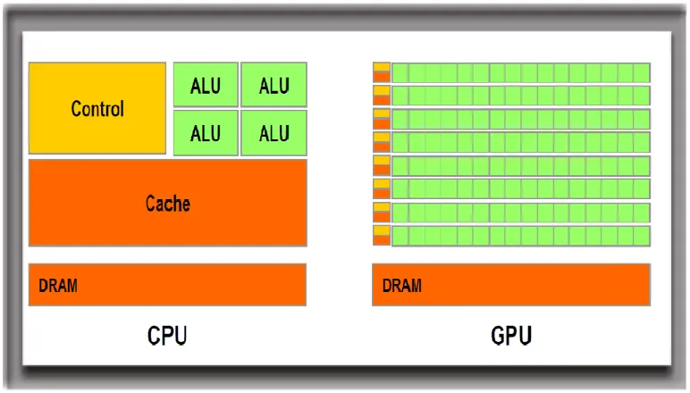
Figure 1.1 Design difference between CPU and GPU
Different from the general purpose processor CPU (Central Processing Unit), which consists of few strong cores and excels in sequential serial processing, GPU has a massively parallel architecture featured by thousands of smaller but efficient cores designed for handling multiple task simulta-neously. In GPU, about 80% of transistors are devoted to data processing rather than data caching and flow controlling, this design leads to more computing power, larger memory bandwidth, and lower energy consumption. Figure 1.1 demonstrates two distinct processor architectures: A CPU has less cores and threads but stronger control and data caching unites that excels in handling complex operations on a single or few streams of data more easily, but cannot efficiently handle large number of streams simultaneously. In contrast, the GPU has more cores and threads but lower clocks frequency and lack of the capabilities for modern operating systems serial tasks, such as branching, file operation, memory management, network processing, et cetera. Thanks to GPU’s special design and architecture, the usage of GPU has been substantially broadened, from pure gaming device to a general purpose solution for intensive computation situations.
Table 1.1 Latest CPU and GPU processor specifications comparison (Oct 2016)
Product name Cores Base Clock (GHz) Micro-architecture Price (dollars)
Intel Xeon E7-8890 v4 24 2.2 Broadwell 7174
NVIDIA GTX TITAN X 3072 1.00 Maxwell 1090
NVIDIA Tesla M60 2x2048 0.90 Maxwell 4600
Radeon R9 390X 2560 1.02 Grenada 490
AMD FirePro S9170 2816 0.93 Grenada 3400
4096 cores and sells at 4600 dollars. Aiming at the promising high performance computing market, lately AMD released the new member of FirePro S series: S9170 with an unprecedented 2.62 trillion floating point operations per second (TFLOPs), making it the fastest single GPU card on the market. Architecturally, GPU is most suited to computation intensive and parallelizable operations such as video processing and physics simulations. For instance, in Adobe vector graphics editor Illustrator CC, which was released on late 2015, GPU function has been available for both Mac OS and Windows versions, and the software works with various GPUs products.
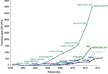
Figure 1.2 shows the evolution of theoretical performance peak for NVIDIA GPU and Intel CPU from 2000 to 2014. Horizontal axis represents the time and vertical axis is the theoretical performances measured by gigabyte floating point operations per second (GFLOPs). GPU and CPU performances was racing neck to neck until early 2004, when the dominant GPU manufacture NVIDIA released the GeForce 7800 GTX with almost 100 GFLOPs, whereas the CPU competitor Prescott has only less than 50 GFLOPs. The performances of GPU and CPU diverged dramatically after 2005, as the number of cores for GPU kept increasing exponentially. For example, for single precision, NVIDIA GTX TITAN has 4,500 GFLOPs versus the INTEL Haswell’s 500 GFLOPs. The gap between GPU and CPU has been growing constantly over time for both single and double precision. Till the end of 2014, GeForce GTX Titan already had 9 times more GFLOP than Intel Haswell CPU. The situation is similar in double precision situation, where NVIDIA Tesla K20x almost triples the performance of Intel CPU at 2014. Based on the long-period trend, the conclusion of even larger difference in the future is almost guaranteed as the Moore’s law has been dying for the last couple years.
As the potential of GPU has been explored and utilized gradually, scientists and researchers are pushing the application of GPU to a new level: general purpose GPU (GPGPU) computing.
1.2
GPGPU computing
Khronos Group. This open standard framework targets an even broader market: heterogeneous systems including CPU, GPU, digital signal processors (DSPs), field-programmable gate arrays (FPGAs) and other processors or hardware accelerators. Its implementations are widely available from large number of famous hardware vendors, for example AMD, Apple, IBM, Intel and even the competitor NVIDIA.[35]
Nowadays, GPGPU-accelerated computing has gained more and more popularity among all kinds of circumstances, for example, scientific, analytic, engineering, consumer and even enter-prise applications. Different from CPU that consists of a few cores optimized for sequential serial processing, GPGPU has a massively parallel architecture consisting of thousand of smaller but more efficient cores designed for handling multiple tasks simultaneously. The relative simplicity of the GPU architectures, combined with the large number of parallel processing units makes GPU as a strong and cost-friendly computing platform for scientific computing.
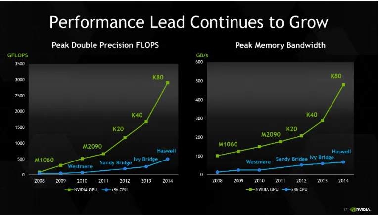
Figure 1.3 Performance comparison NVIDIA Tesla vs Intel x86
GPUs have been gaining larger lead of performance over CPU counterparts over time. For example, Tesla K80 outperformed Intels Haswell CPU for 6 and 8 times in FLOPs and memory bandwidth respectively on 2014. Besides the deep performance advantage, GPU also sever as a low-cost solution for high performance computing market.
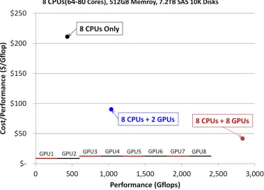
Figure 1.4 Cost comparison between GPU and CPU systems
Figure 1.4 represents the cost-performance ratio, measured by system cost (dollars) divided by GFLOPs[47]. If a pure 8 CPUs system is employed, the ratio is over 200 and performance is less than 500 GFLOPs. On the other hand, by adding 2 GPU to the system, the ratio drops significantly to less than 100 and the performance doubles to over 1000 GFLOPs. Furthermore, by making the GPU and CPU even, 8 GPU and 8 CPU, the ratio can be narrowed down to less than 50 and the overall performance can achieve almost 3000 GFLOPs.
example, Bloomberg shifted one bond pricing application running on 2,000 CPUs to a 48 GPU rack of NVIDIA Tesla GPUs. The CPU system costed $4 million with $1.2 million in annual energy bills whereas the Tesla system costed under $150,000 with about $30,000 yearly in energy. Same story, the French bank BNP Paribas swapped out a 64 CPU system for a pair of NVIDIA Tesla systems and cut daily energy use from 44 kilowatts to 2.9 kilowatts[13].
The two leading manufacturers in discrete GPU market, NVIDIA and AMD (ATI division) together, has taken over 99 percents of the entire booming market. According to Jon Peddie Research report [12], NVIDIA’s market share peaked out in Q3 2015 by taking 81.1% of the discrete GPU market. Seeing the rapid growth in GPGPU market, the dominant CPU manufacture Intel released its own co-processor line called Xeon Phi to compete with NVIDIA and ATI in this increasingly hot market. Different from GPU structure, Intel’s co-processor Xeon Phi has less but faster cores with larger memory and bandwidth. In terms of the usability, as an x86 SMP-on-a-chip architecture, Xeon Phi offers the full capability to use the same tools, programming languages, and programming models as a regular Intel Xeon processor. Specifically, tools like Pthreads, OpenMP, Intel Cilk Plus, and OpenCL are readily available. By avoiding the complicated GPU programming, there is possibility that Intel Xeon Phi could become an easy but competitive scientific computing platform in the near future. The current high performance computing market, however, is still witnessing GPU’s victory.
1.3
GPU vs CPU in parallel computing
1.4
GPGPU programming platforms
CUDA and OpenCL are two prevailing GPGPU frameworks in current market. As an open source and cross-platform GPGPU platform, OpenCL was not fully developed until 2009. It is well-known for heterogeneous computing for different processors including CPU and GPU, and has been actively supported on Intel, AMD, NVIDIA and even Apple system. On the other hand, the dominant proprietary frameworks, NVIDIA’s CUDA, only works with its own GPU product lines (GeForce, Tesla and Quadro). However CUDA was specially designed for GPGPU and parallel computing purpose and it has been proved to run the GPU code significantly faster than OpenCL on NVIDIA devices.
Table 1.2 Performance comparison CUDA versus OpenCL on NVIDIA’s device
End to End running time comparison
CUDA OpenCL
size (Qubits) avg (sec) sd avg (sec) sd
8 2.94 0.007 4.28 0.164
16 5.39 0.008 7.45 0.023
32 10.16 0.009 12.84 0.006
48 17.75 0.013 26.69 0.016
72 32.77 0.025 54.85 0.103
96 76.24 0.033 92.97 0.064
128 123.54 1.091 142.92 1.080
Figure 1.5 Popularity comparison in academia CUDA vs OpenCL
to use CUDA is convenient, with comprehensive online training available as well as other resources, such as webinars and books. Over 400 universities and colleges start to offer CUDA programming courses, including dozens of CUDA Centers of Excellence and CUDA research and training centers. Second, the significant performance difference between CUDA and OpenCL in scientific computing. This is not a surprise that NVIDIA’s CUDA has the better performance on its own GPU products. On the other hand, the discrete GPU market competitor AMD’s GPUs use Very Long Instruction Word (VLIW) structure, that works well for graphics but not great with GPGPU. It requires very strong compiler support that AMD’s OpenCL implementation fails to provide. Finally, thanks to the early adoption of CUDA, there are more tools and libraries available for CUDA than OpenCL. Till the latest version (7.5 for CUDA and 2.1 for OpenCL), NVIDIA CUDA has significantly more resources and better compatibility than its competitor OpenCL, although the later has been catching up lately. For example, CUDA toolkit 8.0 has over 26 officially released libraries including cuBLAS, cuFFT, cuRAND, cuDNN whereas the OpenCL’s counter part clBLAS and clFFT were not available until late 2013. Also, there are still some useful CUDA libraries do not have their counterparts in OpenCL, like Thrust, cuDNN and cuSparse, which is popular to tackle the sparse matrix problems. Also, the NVIDIA has provided a series of useful tools in the CUDA toolkit for developers including a compiler, math libraries and debugger, optimizer as well as elaborated code samples, programming guides, user manuals, and API references.
CHAPTER
2
STATISTICAL METHODS THAT BENEFIT
FROM GPGPU
2.1
GPGPU computing in statistics
GPGPU was already capturing the attention of researchers in many fields before the statistician eventually realized its power. Early applications are primarily found in computer sciences related areas like signal and image processing and visualization[35]. Later on, as adoption in dynamic simulation in physics shows substantial gain in computational efficiency, statistical researchers gradually embrace this new direction.
shows a surprising 100 fold speedup. The computational burden of statistical phylogenetics problem can also significantly reduced by applying parallelized calculations on GPU[43]. In addition, high dimensional optimization problems such as non-negative matrix factorization, PET image recon-struction and multidimensional scaling were all shown to benefit vastly (100 fold speedup) from the GPU utility[gpuahdo]. Due to the parameters separation attribute, majorization-minimization (MM) algorithm has became an ideal match for GPU computing, which has been proved to be highly efficient in high-dimensional challenging and otherwise impossible optimization problems, like high-dimensional fused least absolute shrinkage and selection operator (LASSO) regression[48], geometric and signomial programming[22].
In machine learning, another example is the key statistical method principal component analysis (PCA) for multivariate data analysis based on Gram-Schmidt orthogonalization (also known as GS-PCA). The GPU accelerated algorithm and implementation was introduced on 2008, which yields a 12 fold speedup compared to the CPU version[2]. On the other hand, CUDA based support vector machine package GPUSVM shows a 81-138 fold speed gain by applying CUDA cuBLAS library on the classification method support vector machine (SVM)[25]. Furthermore, as the hottest area in machine learning, Deep Neural Networks (DNNs) is well known for large amounts of computation [32], especially during the training step that may rang from days to weeks. Due to the nature of problem (repeat of identical operations), DNNs has became another popular application in both academia and industry[20] [45].
2.2
Statistical problems that benefit from GPU
Due to the special structure of GPGPU, two big categories of mathematical operations can benefit from GPGPU computing the most: basic linear algebra subprogram (BLAS) and random number generator (RNG). In the following part, we will identify several classes of statistical methods or algorithms that are potentially GPU acceleratable.
2.2.1 GPU accelerated BLAS
which take cubic times and not formally published until 1990, are specialized in matrix matrix operations such as matrix matrix multiplication and symmetric rankk update.
2.2.1.1 Maximum likelihood estimation
The estimation methods of interested parameters can be diverse due to different natures of para-metric models. For example, the classical maximum likelihood estimation (MLE) for frequentist inference maximizes the log likelihood function based on viewed data; The method of moments approximates the expectation by sample means and solves a system of equations. Penalized regres-sion maximizes the log likelihood plus a given penalization terms. All of the above examples falls into the optimization category that ultimately leading to basic linear algebra computation. Take the simplest least square regression method as an example, the computation part boils down to calculate matrix-matrix and matrix-vector multiplication,βbosl= (XtX)−1Xty, which easily extends to
penalized regression withL2 term (Ridge) solutionβbridge= (XtX+λI)−1Xty.
If no closed form solution available and numerical method needs to be applied, GPU-based BLAS can also be more efficient and convenient. LetX1, ...,Xnbenindependent random variables such
that the probability density ofXi isfi(x;θ), which depends on the parameterθ. Then the maximum
likelihood estimator ˆθcan be obtained by maximizing the following log likelihood function
l(θ) =
n
X
i=1
logfi(xi;θ).
By applying one of the most popular gradient methods Newton-Raphson, we have the iterative formula as follow
ˆ
θ(k+1)=θˆ(k)−H(θˆ(k))−1g(θˆ(k)),
where the Hessian matrixH(θˆ)is the matrix of second-order derivatives of the objective functionl(θ) with respect toθevaluated at ˆθ(k), and gradient vectorg(θˆ(k))is the first order partial derivatives. This
procedure involves evaluation of same objective function (usually Gaussian distribution density function) for numerous points and solving the system of linear equation when computing the Newtonian directionH(θˆ(k))−1g(θˆ(k)), which is basically matrix vector operation from level 2 BLAS
category.
In practice, Quasi-Newton method abandons the time-consuming evaluation of Hessian matrix
matrix inversion. For instance the Hessian matrix inversion approximation isHk+1=Hk+∆
xk∆xtk ∆xt
kyk −
HkykyktHk
yktHkyk in DFP method, andHk+1=
I −∆xky t k ytk∆xk
Hk
I −yk∆x t k ykt∆xk
+∆xk∆xtk
ytk∆xk in BFGS. The above two update formulas only contain vector vector and matrix vector basic algebra and vector element-wise operation.
2.2.1.2 EM algorithm
Expectation Maximization (EM) algorithm is a specialized approach designed for MLE problems. By introducing latent variable, EM algorithm does neither require the analytic expression of the log likelihood function nor of the gradient, which makes it a "black box" method. In the Expectation step, we calculate the expected value of the log likelihood function with respect to the conditional distribution of latent variable given observed data under the current iterate of parameter. In the Maximization step, we maximize the expected complete log likelihood with respect to the parameter to be estimated. We keep repeating both the E and M step until the convergence criterion satisfied. One big drawback of EM algorithm is that the rate of convergence can be extremely slow, which has been shown to be linear with rate proportional to the fraction of information about parameter in the observed log likelihood function[9].
SupposeXis the observed variable andZis the introduced latent variable,θ is the unknown parameter. We have the likelihood function of complete-data as
L(θ;X,Z) =p(X,Z|θ).
The MLE of the unknown parameterθcan be obtain by maximizing the log likelihood function with respect to parameterθ
ˆ
θ=arg max
θ logp(x|θ),
where xis the realization of random variableXand the marginal likelihood functionp(x|θ) = P
z
p(x,z|θ) =P
z
p(z|θ)p(x|z,θ).
random variable), which yields the following inequality
logp(x|θ) =logX z
p(z|θ)p(x|z,θ)q(z) q(z) =log Eq
p(z|θ)p(x|z,θ)
q(z)
≥Eq
logp(z|θ)p(x|z,θ) q(z)
.
The third inequality can be derived by applying the convexity of logarithm function and Jensen’s Inequality. Omitting the irrelevant terms we have the Expectation step as
Q(θ|θ(k)) =EZ|X,θ(k)[logp(X,Z|θ)]. The following Maximization step is
θ(k+1)=arg max θ
Q(θ|θ(k)).
Both the E and M step are idea targets for massive GPU parallel computing since they both involve basic linear algebra operations and large number of same function evaluations.
We will show the usage of GPU computing in the most common EM algorithm application: finite mixture model. Suppose we have an random sampleYj from the mixture model, and the density
can be written as
f(yj) = g
X
i=1
πifi(yj),
where thefi(yj)are densities and theπi are mixing proportions that are non-negative quantities
and sums to one
0≤πi≤1
and
g
X
i=1 πi=1.
In many application, the componentsfi(yj)are specified to belong to some parametric family. In
this case, the component densities fi(yj)can be specified as fi(yj;θi), whereθi is the vector of
density as
f(yj;Ψ) = g
X
i=1
πifi(yj;θi),
whereΨcontaining all the unknown parameters in the mixture model and can be written as
Ψ= (π1,π2, ...,πg−1,ξ).
Hereξis the vector containing all the parameters inθ1,θ2, ...,θg. Suppose we havenrandom sample
yj from this mixture model, then we have the likelihood function as
f(y;Ψ) =
n
Y
j=1
g
X
i=1
πifi(yj;θi).
By taking logarithm, we have the following log likelihood function
`(y;Ψ) =
n
X
j=1 log(
g
X
i=1
πifi(yj;θi)).
Typically, EM algorithm is applied to this MLE estimation problem by introducing the missing data that is the knowledge of which group each sample in the data came from. For example, the latent variablesZcan be defined as
Z= (Z1,Z2,Z3, ...,Zn),
where thenis the number of sample size. Then singleZiwill be a vector of sizeg
Zi= (Zi1,Zi2,Zi3, ...,Zi g),
hereg is the number of mixture components. The value ofZi j is defined as
Zi j=
1 ifYj from component i
0 otherwise
.
The values of theZi jare unknown, and are treated by EM as missing information to be estimated
along with the parametersθ andπi of the mixture model.
proportionπi, that is
P(Zi j=1|θ,π) =πi, where 1≤i≤g.
Then we have the complete data log-likelihood function
`(y,Z;Ψ) =
n
X
j=1
g
X
i=1
Zi jlog(πifi(yj;θi)).
The expectation of log likelihood function can be obtain by
Q(θ|θ(t)) =Eθ(t)[`(y,Z;Ψ)|Y=y] =
n
X
j=1
g
X
i=1
pi j(t)log(πifi(yj;θi)), (2.1)
where
pi j(t)=Pθ(t)(Zi j=1|Yj=yj) = π
(t)
i fi(yj;θ( t)
i )
Pg
r=1π (t)
r fr(yj;θ( t)
r )
. (2.2)
Pθ(t)(Zi j=1|Yj =yj)is the posterior probability of individualjcoming from componenti, given
the currentθ(t)and observed datayj. Posterior probability calculation (E step) involvesntimes
g density function evaluations, which could be computationally expensive in genetic or image processing problems due to huge data size. Fortunately, the identical form of PDF function enables the GPU’s Single Instruction, Multiple Data (SIMD) scheme to contribute in this case. For example, the GPU version of normal density function outperforms CPU version over 30 fold in runtime for data size 107. Also the GPU element-wise vector multiplication and vector summation, both exist heavily in posterior probability calculation, present 10 and 8 fold speedup for data size 107 respectively in our testing system (Intel(R) Xeon(R) CPU X5650 @ 2.67GHz with Tesla M2070Q). For the M step, which is maximizingQ(θ|θ(k)), we have already shown the GPU’s usage in typical optimization scenario. Usually, by choosing a proper missing data structure, the M step can be solved analytically. For example in Gaussian mixture problems, the M step boils down to weighted means and variance whose GPU versions yield 8 and 10 fold speedup respectively for data size of 107.
2.2.1.3 MM algorithm
of computations such as nonlinear algebra. If we can, by applying some techniques, convert the complicated computation step into some simpler sub-problems, the efficiency of GPU computing can be pushed to its limit. Here we will introduce the MM algorithm, which can be viewed as an generalization of the famous EM algorithm.
The basic idea of MM algorithm is straightforward. Instead of optimizing the original objective function, we build a surrogate function (majorizing or minorizing) with nicer property, for example separation of parameters that is essential for future GPU application, and then we iteratively update the parameters on the surrogate function.
A functionM(θ|θm)is said to minorize the function f(θ)atθm, if the following conditions satisfied
f(θ)≥M(θ|θm) for all θ and f(θm) =M(θm|θm).
Maximizing the minorizing functionM(θ|θm), we will have the next pointθm+1. By the definition of MM function, we have the ascent monotone property that guarantees the objective function value keeps going up every iteration step
f(θm+1)≥M(θm+1|θm)≥M(θm|θm) =f(θm).
It can be shown that as the most widely applied statistical methods of MLE, expectation-maximization (EM) algorithm is just a special case of MM algorithm by choosing a surrogate function in the E step by using Jensen’s inequality and the convexity of negative log function. Different from EM algorithm that requires building the conditional expectation structure, MM relies on applying inequality to construct the surrogate function. Typically, in EM algorithm, we need to solve nontrivial optimization problem in the M step whereas by choosing a proper surrogate function, the MM algorithm can only consists of basic linear algebra. Furthermore, by applying the MM algorithm, the parameters to be estimated could be completely separated, which is the requirement for the GPU technique comes into play bacause of the limited memory resources in modern GPGPU devices.
Take the classical linear regression as an example. Suppose we have response variabley, and covariatesX, whereXis ann×p design matrix,p is the number of parameters, vectorsyandβ are nandpdimensional respectively. We want to minimize the objective function
n
X
i=1
(yi−xitβ)2
with respect toβ. The traditional solutionβb= (XtX)−1Xty involves matrix inversion, which has
objective function that yields the following majorization function
n
X
i=1
(yi−xtiβ)2≤ n
X
i=1
p
X
j=1 ai j
yi−
xi j
ai j(βj−β (k)
j )−x t iβ(
k)
2
=g(β|β(k)),
wherekis the iteration number, and the equality holds whenβ=β(k). The surrogate function are derived by using the convexity of original objective function. Here we choose have all the constants ai j ≥0, and
Pp
j=1ai j=1. Taking derivative with respect toβ, we obtain the updates as
β(k+1)
j =β
(k) j +
Pp
i=1xi j yi−xtiβ(k)
Pp
i=1
xi j2 ai j
.
For simplicity, we can choose the constants as
ai j=
|xi j|
Pp
l=1|xi l| .
Computationally, for smallp case this iterative scheme is inferior to least square closed form solution. It contains, however, only simple linear algebra and successfully avoids the notorious matrix inversion. In fact, if we can convert complex computing step, for instance matrix inversion, into several simpler sub-problems, the overall computational performance can be hugely improved by applying the massively parallel GPU computing technique.
Another MM algorithm example is linear logistic regression. Suppose we observe a sequence of independent Bernoulli trails withith success probability as
πi(β) =
extiβ 1+extiβ
,
then the likelihood function can be written as
L(β) =
n
Y
i=1 πi(β)yi
1−πi(β)
1−yi .
Typically, we apply the Newton Raphson method to maximize the log likelihood function
l(β) =
n
X
i=1
yilogπi(β) + (1−yi)log(1−πi(β))
which involves the computationally intensive Hessian matrix evaluation and inversion at every iteration. On the other hand, we can transform the problem to a much simpler iterative scheme by applying MM algorithm. Inspecting the second derivative
d2l(β) =−
n
X
i=1 πi(β)
1−πi(β)
xixti,
we find the log likelihood function is concave and a minorizing function is needed in this case. By applying the second order Taylor expansion and inequalityπ(1−π)≤14, we have the following minorizing quadratic function
l(β(k)) +d l(β(k))(β−β(k)) +1
2(β−β
(k))tB(β
−β(k)),
where
d l(β(k)) =
n
X
i=1
(yi−πi(β))xi
t
is the score vector (row vector) and matrixBis defined as
B=−1
4
n
X
i=1 xixit.
The MM algorithm update does involve inversion of the matrixB, but we only need to invert it once and reuse it for every iteration. This logistic regression example demonstrates the attribute of MM algorithm, converting complicated mathematical operation into much simpler linear algebras and separating the parameters and data.
We will provide several case studies to show the power of GPU-MM algorithm combination in chapter 4.
2.2.1.4 Principal component analysis
Principal Component Analysis (PCA), one of the most popular statistical dimension reduction methods, is widely used in areas such as visualization, data compression and feature extraction. Unfortunately, PCA becomes less preferred in large data analysis due to the expensive computation. That is why more computationally efficient approach is always desirable.
Decomposition (SVD). A SVD of anmbynmatrixXis any factorization of the form
X=UΣVt,
whereUismbymorthogonal matrix,Visnbynorthogonal matrix andΣis a diagonal non-negative mbynmatrix. Since the symmetric covariance matrixXXt is diagonalizable, it can be written as
XXt =WDWt. We applying the SVD on matrixXand obtain
XXt=UΣVt UΣVtt. Because matrixVis orthogonal, we have the PCA result as
XXt =UΣ2Ut.
As the original algorithm for PCA, SVD readily fits into the GPU parallel computing framework. There have been many efforts towards SVD algorithms in GPU. Novakovi´c & Singer[31]implemented One Sided Jacobi method for SVD on GPU via CUDA. Bondhugula et al.[3]applied GPU computing technique to improve the diagonalization step by a hybrid GPU based system. Lahabar & Narayanan [21]presented an implementation Golub-Reinsch (Bidiagonalization and Diagonalization) algo-rithm on GPU. In large data sets situation, iterative PCA algoalgo-rithms are more efficient to standard SVD, which extracts all the principal components simultaneously. Nonlinear iterative partial least squares (NIPALS), which performs regressions repeatedly until convergence, matches perfectly with GPU framework. Furthermore, Andrecut[2]implemented both NIPALS and Gram-Schmidt PCA algorithm on GPU via CUDA, which yields 12 fold speedup for a 104matrix factorization problem.
2.2.1.5 Neural networks
networks are organized into three main parts: the input layer, the hidden layer and output layer. Suppose we have ann×kdimensional input matrixX= [x1,x2, ...,xn]t, wherexi= [xi1,xi2, ...,xi k].
If we havepneurons in hidden layer, then we will have anp×nweight matrixW. The neuron output of this hidden layerR=r1,r2, ...,rp
t
can be calculated as the matrix multiplication between input matrix and weight matrix followed by a non-linear activation functionf
R=f (W×X).
For example, we consider an activation function of a bias factor addition and sigmoid operation. Then output matrix can be calculated by
R=sigmoid(M) =
1+e−m11 1+e−m12 1+e−m13 . . . 1+e−m1k 1+e−m21 1+e−m22 1+e−m23 . . . 1+e−m2k
..
. ... ... ... ...
1+e−mp1 1+e−mp2 1+e−mp3 . . . 1+e−mp k ,
where themi j is the element of matrixM=W×X+Band thep×k MatrixBis the bias factor matrix
that can be written as
B=
b1 b1 b1 . . . b1 b2 b2 b2 . . . b2
..
. ... ... ... ... bp bp bp . . . bp
.
Figure 2.1 Neural network structure with single hidden layer
2.2.1.6 Fourier transform
Fourier transform, one of most famous mathematical tools, has been widely applied to various fields such as differential equations, numerical analysis, probability theory, number theory and time series. By transforming complex mathematical operation like differentiation and convolution into simpler operation like multiplication, we can solve the problem in much simpler form and then invert the solution. One of Fourier transform application in statistics is characteristic function of probability density. Supposef(x)is a probability density function, then the characteristic function can be computed by
ˆ f(y) =
Z ∞
−∞
ei y xd x,
The commonly used Fourier transform algorithm is Fast Fourier Transformation (FFT), which rapidly computes the Discrete Fourier transform (DFT) of a sequence. The FFT completes the transformations by factorizing the DFT matrix into a product of sparse factors, which lowers the complexity of computing fromO(n2)toO(nlogn)[46]. As the data size increases dramatically nowadays, however, computation of FFT can still be troublesome in terms of the efficiency. There has been a large number of FFT related studies refer to the GPU utilization. For example Moreland & Angel[28]synthesizes an image by conventional means, performs the FFT, and inverses FFT within 1 second for a 512 by 512 image by using a commodity GPU. Chen et al.[7]achieved 7 fold speedup with respect to Intel MKL for 4096 3D single-precision FFT on a 16-node cluster with 32 GPUs. To help researchers to utilize the power of GPU in FFT, NVIDIA released an official library named cuFFT in the CUDA toolkit[33], which is ten time faster than its counterpart in Intel’s MKL.
2.2.1.7 Batched operation
Figure 2.2 Batched version matrix multiplication
2.2.1.8 Sparse linear algebra
Figure 2.3 Sparse matrix operation performance comparison
Picture 2.3 shows the performance comparison of GPU verse CPU in the case of sparse matrix with dense vector operation. Known as one of the fastest commercial mathematical kernel library, Intel’s MKL’s performance is easily beaten by NVIDIA’s free GPU library cuSPARSE over 5 fold in most of functions. Besides the classes of problems mentioned above, there are still many candidates with potential leading to GPU computing resources such as variable selection, supervised classification and hypothesis testing. In fact, any statistic algorithm will finally reform itself to the brick of math related fields: linear algebra, which can always benefit from parallel computing technique to different extents depending on the nature of problem and size of data.
2.2.2 GPU accelerated random number generator
Besides the linear algebra operations, random number generators (RNG) also has been playing an essential role in all kinds of statistical studies. With the GPU accelerated RNG, some statistic research, which typically suffers from slow running time due to heavy RNG involvements, would be boosted significantly.
2.2.2.1 Monte Carlo simulation
numbers are commonly generated from same distribution with same parameters. A typical Monte Carlo simulation involves three major steps: generating independent data sets; computing the numerical values of the estimators or test statistics for each data set; estimating the parameters or statistics based on the result from last step. Computationally, the first two steps combined dominates the entire simulation study, which can be classified as RNG and linear algebra task respectively and naturally are ideal targets for GPU computing techniques. There have been numerous statistical Monte Carlo research that take advantage of power of GPU. For example, Preis et al.[36]conducted Monte Carlo simulations of the two and three dimensional ferromagnetic lattice Ising models via a variant of the checkerboard algorithm, which yields 60 and 35 fold speedup respectively compared to traditional CPU method. Alerstam et al.[1]applied GPG technique in photon migration simulation study that results in over 1000 fold speedup.
2.2.2.2 Importance sampling
From a statistical simulation perspective, integration via classical Monte Carlo and importance sampling are ideal computational tasks for the GPU. This is because each thread can produce and weight a sample in parallel, assuming that the sampling procedure and the weighting procedure have no conditional branches. If these methods have branch, performance would be hugely compromised because many threads are waiting idly for other threads that are still running. This can occur, for example, if the sampling procedure uses rejection sampling. In Bayesian inference, many problems can be described as sampling from a probability distribution whose densityπcan be computed pointwise. Suppose we are interested in the expectation of given functionθ, which be written as
I =
Z
x
θ(x)π(x)d x.
Then the Monte Carlo estimation of the integral is given by
ˆ IM C =
1 N
N
X
i=1 θ(x(i)),
wherex(i)Ni=1are samples from density functionπ
can be sampled from easily and estimate the integral via
ˆ II C =
1 N
N
X
i=1
W(i)θ(x(i)).
The importance weightsW(i)can be obtained by
W(i)=PNw(x(i))
i=jw(x(j))
,
where
w(x(i)) =
π(x(i)) γ(x(i)).
We can easily find that the important sampling is a perfect match for GPU’s SIMD concept: sampling from certain distribution, evaluating same objective function at different points and simple linear algebra, which is exact what we have been discussing previously.
2.2.2.3 Markov chain Monte Carlo
Another approach of sampling fromπis the famous Markov chain Monte Carlo (MCMC) method. Instead of finding a nontrivial importance density function that is supposed to attain reasonable variance of estimate with practical value of sample sizeN, MCMC method constructs an ergodicπ stationary Markov chain sequentially. All the samples are drawn from the dependent Markov chain iterations, and the estimate can be obtained from the sample path. Sometime, however, the slow convergence rate of MCMC method makes it an extraordinary computation burden. Let us consider a multivariate normal mixture models under truncated Dirichlet process (TDP) priors. Suppose we have apdimensional random data vectorxwith density function
g(x|Ψ) =
k
X
j=1
πjN(x|µj,Σj),
where parametersΨ={π1, ...,πk,µ1, ...,µk,Σ1, ...,Σk}for a fixed constant group numberk. The TDP
analysis uses normal- inverse-Wishart priors for normal component parameters, that is
For the mixture probabilities parametersπj, we follow the beta prior for DP model, that is
πj =
v1, if j=1 vj
Qj−1
r=1(1−vj), if j=2 :k−1
1, if j=k
, (2.3)
where vj ∼ Beta(1,α) for j = 1, 2, ...,k −1 and the DP precision parameterα has a
condition-ally conjugate gamma prior. MCMC algorithm repeatedly resamples values of parametersΨ =
{π1, ...,πk,µ1, ...,µk,Σ1, ...,Σk}of thek normal components[44]. Each MCMC iteration has
follow-ing steps
1. Recompute configuration probabilities:
Calculateπj(xi) =P(zi=j|xi,Ψ) =πjN(xi|µj,Σj)/g(xi|Ψ), wherei=1 :nandj=1 :k.
2. Resample configuration indicators:
Makenindependent and individual multinomial draws of size 1,(zi|xi,Ψ)∼Mn(1,π1:k(xi)).
Then compute the counts ofnpoints amongk components,nj =#{zi = j,i =1 :n}for
j=1 :k.
3. Resample means and covariance matrices:
Draw new normal parameters(µj,Σj)independently overj=1 :k from implied conditional
normal-inverse-Wishart distributions base on the currently allocated data.
4. Resample mixture weights:
Draw independent beta variatesvj ∼Beta(1+nj,αj), whereαj =α+
Pk
r=j+1nr. Then
recom-pute the mixture probabilitiesπ1=v1,vj
Qj−1
r=1(1−vj)forj=2 :k−1.
5. Resample DP precision parameter:
Drawαfrom conditional gamma posteriorp(α|n,Ψ)
CHAPTER
3
R GPGPU SOLUTION
3.1
GPU computing tools for statistics
3.1.1 GPU tools in other languages
As one of the most popular proprietary programming languages in applied math and engineering, MATLAB has successfully embraced GPU computing early on. It has already released 266 GPU build-in functions in the Parallel Computing Toolbox by July 2016, which was built on NVIDIA’s CUDA platform due to its highly enhanced performance and popularity among both academia and industry. MATLAB’s build-in GPU functions include standard BLAS and some of LAPACK functions as well as some element-wise operations like vector logarithm, exponential, et cetera. According to MathWorks GPU computing website, if all the functions that user want to use are supported on the GPU, user can simply transfer input data to the GPU, and retrieve the output data from the GPU after applying GPU functions[38].
users within a short period of time. Formerly known as MATLAB CUDA-enabled GPGPU toolbox Jacket, open source library ArrayFire, a GPGPU extension for C, C++and Fortran, has been actively deployed in many areas even the American defense industry. It has three different versions, one for CUDA GPU, one for OpenCL GPU and one for regular CPU, which makes the ArrayFire a cross-platform solution for GPGPU computing. Users can easily switch between CUDA or OpenCL without changing the ArrayFire code[26]. Currently, ArrayFire has over 240 highly tuned functions in its latest version 3.4.0, which includes linear algebra, statistics, signal processing and computer vision. Julia has already added ArrayFire into its library collections. Another example of the GPU computing can be found in CUDALink package of Wolfram’s Mathematica, a computer algebra programming language widely used in scientific, engineering, mathematical, and computing fields. Based on NVIDIA’s CUDA, CUDALink provides some of BLAS, FFT, and image processing functions. Overall speaking, as the GPGPU concept gaining its acknowledgment among both academia and industry, more and more programming languages have been making effort to take a share in this promising market by releasing official packages or encourage volunteer’s contributions.
3.1.2 GPGPU computing in R
R is the most popular open source statistical programming language, however most of native R functions involve no parallelism and they can only be executed as separate instances on multicore or cluster hardware for large data-parallel analysis tasks. Unfortunately, few statisticians are trained to program GPU, and consequently may not have full access to the GPU resources like NVIDIA’s CUDA libraries. Currently, there has been plentiful third party CUDA wrappers available for Python, Perl, Fortran, Java, MATLAB and Mathematica, unfortunately there is no one for R that is comprehensive enough to handle practical statistical problem. Some available packages may have some certain functions but not all, that means users have to refer to several different packages to complete one easy calculation.
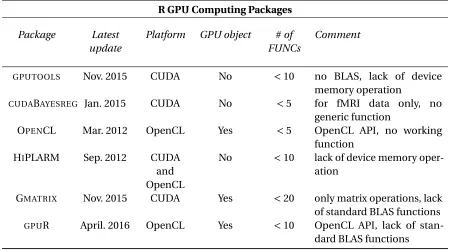
Table 3.1 R GPU computing packages review based on Dirk Eddelbuettel’s CRAN tast view
R GPU Computing Packages Package Latest
update
Platform GPU object #of FUNCs
Comment
GPUTOOLS Nov. 2015 CUDA No <10 no BLAS, lack of device
memory operation
CUDABAYESREG Jan. 2015 CUDA No <5 for fMRI data only, no
generic function
OPENCL Mar. 2012 OpenCL Yes <5 OpenCL API, no working
function
HIPLARM Sep. 2012 CUDA
and OpenCL
No <10 lack of device memory oper-ation
GMATRIX Nov. 2015 CUDA Yes <20 only matrix operations, lack
of standard BLAS functions
GPUR April. 2016 OpenCL Yes <10 OpenCL API, lack of stan-dard BLAS functions
developed via NVIDIA’s CUDA system while two via OpenCL. It partially verifies our conclusion of superior popularity of CUDA in research area. All package maintainers are active except OpenCL and HiPLARM, which were updated on Mar and Sep 2012 respectively. Even though there has been so many packages targeting the same goal, none of them has successfully provided a comprehensive and efficient GPU computing solution that is supposed to cover standard BLAS routines, part of LAPACK and random number generators as well as the performance key: GPU memory operation.
As the first and most popular R gpu computing package,GPUTOOLS[6]was built on the NVIDIA CUDA framework and released the 1.0 version in Nov 2015. However, lack of BLAS functions and random number generators makesGPUTOOLSincapable of dealing with real world problem. In addition,GPUTOOLS’ design requires the unnecessary communication between GPU and CPU. An-other popular packageCUDABAYESREG[40]is problem specific. It implements a Bayesian multilevel
HIPLARM[30]provides a linear algebra solution on heterogeneous architectures based on MAGMA, PLASMA and CUDA. However HIPLARM is clearly insufficient to be a comprehensive solution for
GPU computing in R for couple reasons. First of all, since it was released on 2012 back to when CUDA toolkit was way from being mature, HIPLARM only contains handful of matrix operation functions. Moreover, similar toGPUTOOL, HIPLARM does not provide GPU memory operation interface. Also,
its functions pool is far from practically useful in the view of computing statistician, BLAS and random number generators are totally unavailable in HIPLARM. GMATRIX, based on CUDA and released on Dec 2015[29], is the currently best solution among all the six packages. It successfully provided a GPU interface for user to create GPU object in R system, and it also contains matrix operation functions including addition, subtraction, multiplication as well as some random number generators. But unfortunately there are still some function design issues in GMATRIXpackage. To
mimic the matrix operation habit in R, GMATRIXtotally abandoned the standard BLAS convention, which has been proved highly efficient in the past. For example, when we need to computeAx+b, whereAis a matrix andxandbare vectors, GMATRIXneeds to computeAxand store the result in a intermediate vector and then add to vectorb. On the other hand, in the standard BLAS design, by calling BLAS gemv function, no intermediate vector storage is needed and computing efficiency can be significantly increased. Also, GMATRIXmainly focus on general matrix operation and neglects the need of the element-wise operation and matrix with special structure such as symmetric, banded, triangular as well as batched version of matrix operation, which turns out to be highly convenient in situations such as magnetic resonance imaging (MRI)[15], where billions of 8x8 and 32x32 eigen-value problems need to be solved. Lastly, packageGPUR[10], released on April 2016, is basically an updated version of OpenCL by providing several matrix operation functions. Its disadvantages include lack of BLAS functions and random number generators. After reviewing all the six packages, we find the demand of comprehensive R GPU computing solution has not been perfectly satisfied yet. First, it should be based on CUDA framework considering the performance and popularity in academia. Second, it should enable GPU memory operation, such that intermediate computations may be kept on the GPU and reused. Third, random number generators of popular distributions should be included. Last but not least, package should have as many standard BLAS and LAPACK functions as possible to make it practically useful in practical project, because avoiding the data transferring between GPU and CPU is always desired in GPGPU computing.
have some very useful libraries specialized in scientific computing, including cuRAND cuBLAS, corresponding to random number generator and BLAS functions respectively.
According to Table 3.1, the most noticeable deficiency of current R GPU packages is the inefficient memory management. For example, creating a 108GPU vector costs 0.013 second while transferring it to CPU costs .042 second in our testing system (Intel(R) Xeon(R) CPU X5650 @ 2.67GHz with Tesla M2070Q). Considering the high frequent vectors operation in real problem, the computation efficiency could be dramatically dragged down by those unnecessary memory allocation. Technically, the Peripheral Component Interconnect Express (PCIe) slot (most discrete GPU based on) bandwidth to the main host memory is an order of magnitude lower, for example 20 times for NVIDIA K20X GPU, than the GPU bandwidth to its local memory. Therefore, CPU GPU data transferring might significantly slow down the application, making minimization of communication overhead among the most important optimization goals.
The programming part is highly similar to CPU application, except that we need to allocate the memory on device side to call the CUDA kernels. As an independent component of PC, GPU is separated from CPU and both have their own Dynamic Random-Access Memory (DRAM). Parallel portions of an application are executed on the GPU (also known as device versus CPU as host) as ker-nels. Each kernel is executed at a time but many threads can execute the same kernel simultaneously. Different from CPU, GPU threads are extremely lightweight and have very little launch overhead. In other word, cooperation among all the threads is much more efficient than CPU. For each kernel, a grid of thread blocks will be launched, threads within a block cooperate via shared memory. To tackle the problem of redundant memory operation, in RCUDA we applied a new design. In next section, we will talk about the R GPU computing package design and implementation.
In the following section, we will discuss step by step how we built our R GPU computing package RCUDA. By outlining the technical details, we aim to encourage more statistician to embrace the GPGPU concept and build GPU package for their own computing tasks.
3.2
R GPGPU solution
3.2.1 Package design
There are three major types of overhead in CUDA programs: memory management overhead, memory transfer overhead, and kernel launch overhead.
3.2.1.1 Memory management overhead
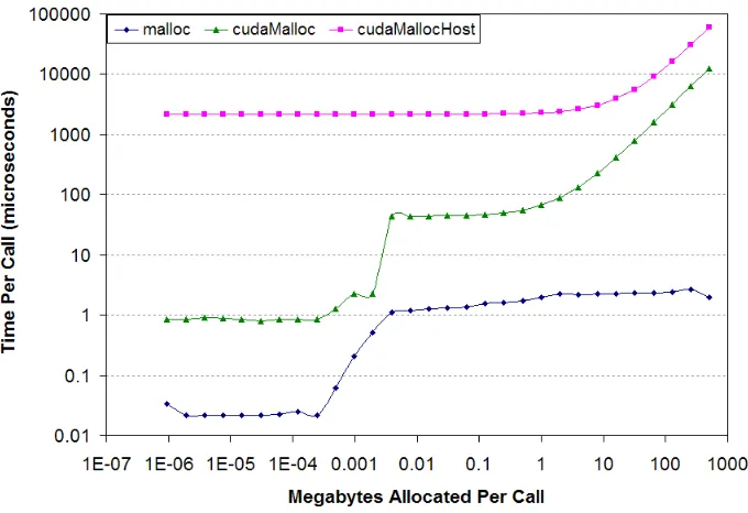
In most programming languages, memory allocation operation is relatively cheap, such as malloc and free in C standard library. However inexpensive memory operation assumption is no longer valid in the context of CUDA. For example, as the counterpart of C function malloc, cudaMalloc call is two orders of magnitudes slower when allocating memory size over 1MB and four orders slower for over 1000MB. And this difference is the same for free and cudaFree comparison.
Figure 3.2 Deallocation time per call as a function of the number of bytes allocated per call[4]
The solution of this problem is to avoid unnecessary memory allocation and reuse the GPU objects as much as possible.
3.2.1.2 Memory transfer overhead
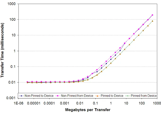
Figure 3.4 Transfer throughput as a function of transfer size[5]
To reduce the severity of memory transfer overhead, the ideal solutions is to keep as much computation on the GPU side as possible and reduce the data transferring between GPU and CPU whenever possible.
3.2.1.3 Kernel launch overhead
Figure 3.5 Time per empty kernel call
Two solutions can be applied to this overhead problem: writing some all-in-one kernels and reduce the total number of kernel calls or launching many asynchronous kernels back-to-back with minimum number of intervening synchronization kernels such as memory transfers. All-in-one CUDA kernel is definitely the best solution in terms of the performance, but it compromises the flexibility and expandability of kernel considering its strong design purpose. Thus, we choose the alternative: by providing plentiful of small but more general asynchronous kernels that can be connected together to solve user’s problem while minimizing the synchronization operations.
After reviewing the currently available R GPU package structure and analyzing the overhead problems discussed above, we finally decided to apply the following design for our RCUDA.
Allocate memory in GPU
memory man-agement overhead
memory transfer
CPU to GPU
transfer overhead
run GPU kernel
kernel launch overhead repeat
3 times
memory transfer
GPU to CPU
transfer overhead
stop
no more kernel more kernel
reuse GPU object
from last step
run GPU kernel repeat
3 times
no kernel launch overhead for
second and later kernels
keep GPU object for next step
stop more kernel
no more kernel
3.2.2 Package building
There are three main steps of using the RCUDA package: creating GPU array by transferring from CPU, running the function on the GPU array, transferring the array back to CPU. Different from CPU programming problem, running any device kernel requires the data to be allocated on the GPU, which means we can not directly apply function on objects created by R. The user need to call a creating function to copy the R vector to GPU memory, apply all the wanted GPU functions on it, and then call another gathering function to transfer the device vector back to R. The output of data creation function is a pointer to memory of GPU, thus user can not apply any R native CPU function to GPU vector without transferring the data back to CPU.
Our R package, RCUDA, is quite different from most currently available packages in several aspects: First, RCUDA is not a package aiming to solve specific problems, it is more of a collection of generic functions and random number generators, and consequently we need to write the package in C and call the external C functions in R; Second, as a portable package, RCUDA requires the C code to be compiled and linked by both CPU and GPU compiler (GCC and NVCC), which means we need to overcome the difficulties caused by mixture of real time compiling; Last but not least, because we want to enhance the computing efficiency as much as possible, pass-by-reference technique has been applied instead of R’s pass-by-values, but this technique also means extensive heavy work in design and implementation.
3.2.2.1 Calling C function in R
As the fundamental unit of shareable code, R package bundles together code, data, documentation, and examples, and is easy to share with others. R packaging system has been one of the key factors of the rapid success of the R project thanks to its easy, transparent and cross-platform extension of the R base system. As the leading statistic language, R CRAN repository features 8331 available packages on Mar 03 2016, many of which are written in R itself that makes it easy for contributors to implement the algorithm and user to understand the procedure. But as an interpreted language, R is notorious for its poor performance in computationally intensive tasks. Thus, R packages that involves large scale data are written in low level languages like C, C++or Python. Here we want to introduce the way of integrate foreign language with R platform.
which can be accomplished by R build-in gcc compiler using R CMD SHLIB command or other compiler specified by makefile. Once the shared object is created, we dynamically load it in R by using dyn.load function and call it with either .C or .Call function. As the one of the two major R’s C interfaces, .C function allows user to write simple C code without too much R data structure knowledge, but its drawbacks are obvious and unnegligible: all memory allocation must be done in R and all arguments are copied locally before being passed to C function that may cause memory bloat. On the other hand, .Call function arranges the heavy memory allocation task to the more efficient C function and does not require wasteful argument copying. However, .Call function requires much more knowledge of R interval data types because all the inputs and outpust of C function will be a R SEXP type, a pointer to a SEXPREC. In the RCUDA package, we will stick with .Call interface.
3.2.2.2 Writing C function for R
Different from .C interface, .Call requires the input and output to be SEXP type:a variant type, with subtypes for all R data structures including numeric vector, integer vector, logical vector, character vector, list, functions and external pointers. Also, we need to protect the item allocated in C to tell R not to garbage collect it by using PROTECT and remove one item from the stack of protected items using UNPROTECT(1). Since we try to avoid unnecessary memory allocation by using pass-by-reference technique, RCUDA’s function input and output are all R external pointer, here is a short example to illustrate the SEXP and external pointer usage.
Sample R code 3.1 Sample C code of GPU object creation in R


![Figure 3.2 Deallocation time per call as a function of the number of bytes allocated per call [4]](https://thumb-us.123doks.com/thumbv2/123dok_us/1484630.1181633/45.612.148.487.112.348/figure-deallocation-time-function-number-bytes-allocated.webp)