Integration of Wind Farm for Maximum Load ability of Power System Using Particle Swarm Optimization

ISSN (Print) : 2347 - 6710

I

J

I

R

S

E

T

2014 International Conference on Innovations in Engineering and Technology (ICIET’14)

On 21st _{& 22}nd _{March Organized by}

K.L.N. College of Engineering, Madurai, Tamil Nadu, India

ABSTRACT—Since DG units have a small capacity compared to central power plants, the impact is minor if the penetration level is low (1%-5%). However, if the penetration level of DG units increases to the anticipated level of 20%-30%, the impact of DG units on voltage stability will be profound.This paper discusses some important aspects related to maximum loadability in electrical power systems. The effectiveness of the analyzed method is demonstrated through numerical studies in IEEE 14 bus test systemand an optimal location of wind farm is determined using particle swarm

optimization.

KEYWORDS: Distributed Generation, maximum loadability, Wind farm, Stability Index, Particle Swarm optimization

I. INTRODUCTION

A traditional electrical generation system consists of large power generation plants, such as thermal, hydro, and nuclear. Because these plants are located at significant distances from the load centers, the energy must be transported from the power plants to the loads through transmission lines and distribution systems. The increase in load demand requires that new generation power plants be built and that the transmission and distribution systems are expanded, neither of which is recommended from an economic or environmental perspective, especially when many countries are trying to meet the targets set in the Kyoto Protocol in order to reduce greenhouse gas emissions [3],[4]. Therefore, interest in the integration of distributed generation (DG) has been rapidly increasing [5]. This is due to the restructuring of electricity and

technological development of small scale power generation.

II. DISTRIBUTED GENERATION

Distributed generation is loosely defined as small-scale electricity generation fueled by renewable energy sources, such as wind and solar, or by low-emission energy sources, such as fuel cells and micro-turbines. IEEE defines DG as “the generation of electricity by facilities that are sufficiently smaller than central generating plants so as to allow interconnection at nearly any point in a power system.” IEEE compared the size of the DG to that of a conventional generating plant. A more precise definition is provided by the International Council on Large Electric Systems (CIGRE) defines distributed generation as “all generation units with a maximum capacity of 50 MW to 100 MW that are neither centrally planned nor dispatched”.

III. VOLTAGE STABILITY

Voltage stability refers to the ability of a power system to maintain steady and acceptable voltages at all buses in the system after being subjected to a disturbance from a given initial operating condition. The main factor causing voltage instability is inability to meet the reactive power demand. At any instant, a power system should operate in a stable manner, thereby meeting operational criteria. In case of credible contingency, the system should be secure. Voltage instability occurs when the receiving end voltage decreases well below the normal value and cannot be restored even after using VAR compensators.

Integration of Wind Farm for Maximum

Load ability of Power System Using Particle

Swarm Optimization

A.Marimuthu#1, B.Kumarasamy*2

#1 Associate Professor, Department of Electrical and Electronics Engineering, K.L.N. College of Engineering,

Madurai, Tamil Nadu, India.

*2PG Scholar, Department of Electrical and Electronics Engineering, K.L.N. College of Engineering, Madurai,

Copyright to IJIRSET www.ijirset.com 366 Nowadays power systems are operating close to their

stability limits because of constraints imposed by economy and environment. So we face a challenge in maintaining a stable and secure power system operation. The process by which the voltage drops to unacceptable value due to avalanche of events along with voltage instability.The initial event may be due to a variety of causes such as small gradual changes such as natural increase in system load, large sudden disturbances such as loss of a generating unit or a heavily loaded line and also due to cascading events Voltage collapse occurs due to the slow decay in voltage. Once associated with weak systems and long lines, voltage problems are now also a source of concern in highly developed networks as a result of heavier loading. The more the load increases, the more the voltage in the load bus decreases until reaching a critical value that corresponds to the maximum power transfer and is related to voltage instability. Beyond this point voltage, stability is lost and voltage collapse could easily occur.

The study of voltage stability has been analyzed under different approaches that can be basically classified into dynamic and static analysis. The static voltage stability methods depend mainly on the steady state model in the analysis, such as power flow model or a linearized dynamic model described by the steady state operation. The dynamic analysis implies the use of a model characterized by nonlinear differential and algebraic equations through transient stability simulations.

Although stability studies, in general, requires a dynamic model of the power system, in this paper analysis of voltage behavior has been approached using static techniques, which have been widely used on voltage stability analysis.

IV. MODELLING OF WIND TURBINE

Wind turbines are classified into four types: A, B, C, and D. Type A uses a fixed speed wind turbine with a Squirrel Cage Induction Generator (SCIG) connected to the grid via a transformer. In this type, fluctuations in wind speed are converted to electrical power fluctuations and consequently into voltage fluctuations if the grid is weak. Type B uses a Wound Rotor Induction Generator (WRIG). In this type, the slip is typically controlled from 0 to -0.1, meaning that the speed of the generator could be increased up to 10% above the synchronous speed. Type C uses a technology called the Doubly Fed Induction Generator (DFIG) with a wound rotor induction generator (WRIG) and a partial scale frequency converter on the rotor circuit. Type D uses a full variable speed wind turbine with an induction or a synchronous generator, connected to the grid through a full load frequency converter.

For a type C WTGU, the output electrical power

generation is given by

𝑃𝑊 =

0 , 𝑣𝑤 < 𝑣𝑐𝑖𝑛𝑜𝑟𝑣𝑤 > 𝑣𝑐𝑜𝑢𝑡

𝑃𝑟𝑎𝑡𝑒𝑑 𝑣𝑤−𝑣𝑐𝑖𝑛

𝑣𝑁−𝑣𝑐𝑖𝑛 , 𝑣𝑐𝑖𝑛 ≤ 𝑃𝑟𝑎𝑡𝑒𝑑, 𝑣𝑁 ≤ 𝑣𝑤 ≤ 𝑣𝑐𝑜𝑢𝑡

𝑣𝑤≤ 𝑣𝑁 (1)

Wherevcin, vcout, vN are cut-in speed, cut-out speed and

nominal speed of wind turbine respectively. 𝑣𝑤is the

average wind speed. Prated is the rated output power of the

turbine and can be represented by

𝑃𝑟𝑎𝑡𝑒𝑑 = 0.5 𝜌𝐴𝑣𝑤3𝐶𝑝 (2)

Where A is the swept area of the rotor, ρ is the

density of air, vw is the wind speed and Cp is the power

coefficient.

Wind farms have been represented as PV or PQ

models in power flow studies. The main drawback is that the available reactive power range is limited either to a maximum power factor or to a fixed regulation band. The reactive power capability from variable- speed turbines may differ depending on the variable-speed technology. Modern wind units use variable-speed generators connected to the grid by power electronic converters. These converters offer the possibility to control the reactive power output of wind units by varying voltage magnitude and frequency. DFIG is the most popular generators employed in wind units and could offer dynamic reactive power control due to the grid side converters. The main function of reactive compensation devices is to provide voltage support to avoid voltage instability or a large-scale voltage collapse. Variable speed wind turbines offer voltage control capability at the Point of Common Coupling (PCC) by making use of their reactive power injection capability.

V. LOAD FLOW

The state of any power system can be determined using load flow analysis that calculates the power flowing through the lines of the system. The power-flow (load-flow) analysis involves the calculation of power flows and voltages of a transmission network for specified terminal or bus conditions.

The system is assumed to be balanced. Load bus and generator bus are the two main types of buses. Slack bus which is a special type of generator bus is used as reference bus accounts for the losses in the system. Associated with each bus are four quantities: active power

P, reactive power Q, voltage magnitude V, and voltage

angle θ.

Methods used to find load flow for a particular power system are: Gauss-Seidel, Newton-Raphson and the Fast-Decoupled method. Developments have been made for finding power-system load flow solutions for the past few years. As a result of this, reliability and speed of convergence of the numerical solutions has increased.

Copyright to IJIRSET www.ijirset.com 367 size almost linearly while using NR for large networks.

Computing time is reduced remarkably as well as the convergence is ensured. NR method requires only less computing time for network modifications, acceleration factors need not be found out and the choice of slack bus is rarely critical. We can include a wide range of representational requirements such as on load tap-changing and phase-shifting devices, area interchanges, functional loads and remote voltage control easily and effectively using NR method. The NR load flow is well suited to online computation.

VI. PARTICLE SWARM OPTIMIZATION

PSO is a robust stochastic optimization technique based on the movement and intelligence of swarms.PSO applies the concept of social interaction is applied by PSO for solving a problem. James Kennedy (social-psychologist) and Russell Eberhart (electrical engineer) developed PSO in 1995. It uses a number of agents (particles) that constitute a swarm moving around in the search space looking for the best solution. Each particle is treated as a point in an N-dimensional space which adjusts its “flying” according to its own flying experience as well as the flying experience of other particles.

Each particle keeps track of its coordinates in the solution space which are associated with the best solution (fitness) that has achieved so far by that particle. This

value is called personal best, pbest. Another best value

that is tracked by the PSO is the best value obtained so far by any particle in the neighborhood of that particle. This

value is called gbest.

The basic concept of PSO lies in accelerating each particle toward its pbest and the gbest locations, with a random weighted acceleration at each time step as shown in Fig.1

Fig1: Concept of modification of search point by PSO

Where

sk : current searching point.

sk+1: modified searching point.

vk : current velocity.

vk+1: modified velocity.

vpbest : velocity based on pbest. vgbest : velocity based on gbest.

The modification of the particle‟s position can be mathematically modeled according the following equation:

Vik+1 = wVik +c1 rand1(…) x (pbesti-sik) + c2 rand2(…) x (gbest-sik) (3)

Where

vik : velocity of agent i at iteration k,

w : weighting function, cj : weighting factor,

rand :uniformly distributed random number between 0&1, sik : current position of agent i at iteration k, pbesti : pbest of agent i,

gbest: gbest of the group.

VII. OPTIMAL VOLTAGE STABILITY

If the load is to be considered as constant power, then the loadability limit corresponds to the maximum power deliverable in buses.

Voltage stability limits are difficult to obtain by means of the classical load flow methodologies since load flow calculations fail to converge close to the point of voltage collapse (PoC). The classical way to obtain PV and QV curves is by the continuation method which consists of two steps:

1. The predictor step: From an initial operating point, find the next point for a load P increase by estimating the changes in the power flow variables.

2. The corrector step: to solve the power flow equations for the next operating point by using the estimated values obtained at the predictor step as initial values.

Another way of computing the maximum loadability point corresponds to the use of optimization methodologies as the OPF or the heuristic techniques. The optimization problem is implemented to represent properly the power system security to the maximum distance to the voltage collapse.The parameter to be maximized drives the system to its maximum loading condition.

𝑃𝐷= 𝑃𝐷0 1 + 𝜆 (4)

𝑄𝐷= 𝑄𝐷0 1 + 𝜆 (5)

Where the multiplier designating the load change rate is constant in all nodes. Loads in all buses increase proportionally to their initial load levels and the generators outputs increase proportionally to their initial generations too.

VIII. PROBLEM FORMULATION

Objective Function:

The objective is to maximize the loadability limit 𝜆 subject to equality and inequality constraints.

Maximize f(x) = 𝜆 (6)

Subject to 𝑓 𝑥 = 0 𝑔 𝑥 ≤ 0(7)

The constraints are classified as:

Equality Constraints:

A basic equality constraint corresponding to the power flow equations in every bus is:

𝑃𝐺𝑖− 𝑃𝐷𝑖= 𝑃𝐿𝑖𝑘 (8)

𝑄𝐺𝑖− 𝑄𝐷𝑖+ 𝑄𝐹𝐴𝐶𝑇𝑆 ,𝑖= 𝑄𝐿𝑖𝑘 (9)

Bus iis linked to bus kthrough a transmission line whose admittance is:

𝑌𝑖𝑘= 𝐺𝑖𝑘+ 𝐵𝑖𝑘 (10)

Active and Reactive power between buses „i‟ and „k‟ is given by

sk

vk

v_pbest v_gbest

sk+1

vk+1

sk

vk

v_pbest v_gbest

sk+1

Copyright to IJIRSET www.ijirset.com 368

𝑃𝐿𝑖𝑘= 𝑉𝑖 𝑖=1𝑁 𝑉𝑘(𝐺𝑖𝑘cos 𝜃𝑖𝑘+ 𝐵𝑖𝑘sin 𝜃𝑖𝑘) (11)

𝑄𝐿𝑖𝑘= 𝑉𝑖 𝑖=1𝑁 𝑉𝑘(𝐺𝑖𝑘cos 𝜃𝑖𝑘− 𝐵𝑖𝑘sin 𝜃𝑖𝑘) (12)

In-equality Constraints

Network technical constraints: Voltage level at buses is not allowed to be outside the maximum and minimum values according to grid voltage regulations.

𝑉𝑖,𝑚𝑖𝑛 ≤ 𝑉 ≤ 𝑉𝐼,𝑚𝑎𝑥 (13)

Physical limits of generators:

The maximum power injected by wind farms is constrained by the maximum capability of each wind turbine. Active power injected by the turbine will depend on the wind availability for each wind turbine. Active power output is restricted by lower and upper limits, where Pgi,min, Pgi,max are the minimum and maximum operating power respectively:

Pgi,min≤Pgi≤Pgi,max ; i= 1,2,……NG (14)

Qgi,min≤Qgi≤Qgi,max ; i =1,2……NG (15)

Physical limits of FACTS devices:

Reactive power from FACTS devices is restricted by the lower and upper limits:

QFACTSi,min≤ QFACTSi ≤ QFACTSi,max(16)

Wind farm connection point (LocWF) constraints: The potential connection point from the wind farm to the grid is limited to the geographical area in which the available wind resource is higher:

BusLocWFi,min≤ BusLocWFi≤ BusLocWFi,max , i = 1,2,…NG (17)

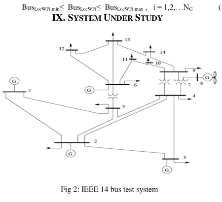
IX. SYSTEM UNDER STUDY

Fig 2: IEEE 14 bus test system

X. RESULTS AND DISCUSSION

The results obtained for load flow of the test system using PSO is presented below:

TABLE I LOADFLOWUSINGPSO

Bus Number

Voltage magnitude (p.u.)

Voltage Angle (deg)

1 1.0600 0

2 1.0450 -4.9897

3 1.0100 -12.7378

4 1.0176 -10.3269

5 1.0194 -8.7863

6 1.0700 -14.2453

7 1.0614 -13.3857

8 1.0900 -13.3901

9 1.0558 -14.9657

10 1.0508 -15.1253

11 1.0568 -14.8179

12 1.0552 -15.1019

13 1.0504 -15.1824

14 1.0354 -16.0619

As a next step the maximum loadability of power systems were calculated using PSO and the results are presented here:

Bus Number

Voltage magnitude (p.u.)

Voltage Angle (deg)

1 1.0600 0

2 0.8510 -8.3031

3 0.5705 -35.5053

4 0.6723 -22.6908

5 0.7141 -17.6695

6 0.6200 -35.7136

7 0.6217 -32.3206

8 0.6037 -32.1306

9 0.6004 -38.4918

10 0.5929 -39.2828

11 0.5982 -38.5942

12 0.5982 -39.2731

13 0.5915 -39.1239

14 0.6000 -40.1070

λ 0.7575

The OPF formulation is applied to a modified IEEE-14 bus power system in which the original synchronous generator in bus 8 has been removed and a wind farm has

been installed with a rated power PWT = 30 MW. Two

different scenarios have been considered:

Scenario 1: The wind farm in bus 8 is adjusted to

maintain a constant power factor, cos θ =1 (QWT = 0).

Copyright to IJIRSET www.ijirset.com 369

Particle swarm optimization technique was

implemented with 50 particles using weighting factors c1

and c2 equal to 2 and the results obtained are discussed

here.

Scenario 1:

TABLE II

COMPARISON OF MAXIMUM LOADABILITY

Voltage profile versus λ load parameter for scenario 1, critical buses are #3, #10, #13, and #14.

Scenario 2:

TABLE II

COMPARISON OF MAXIMUM LOADABILITY

The maximum loadability in scenario 2 increases compared to scenario 1.Scenario 2 involves the reactive injection capability of the wind farm. It can be noted how the reactive power injection at the wind farm terminals improves the system voltage stability

Fig 3: loadability for scenario 1 and 2

XI. CONCLUSION

This paper presents the application of Particle swarm optimization in determining the maximum loadability of power system. It can be noted until what extent wind energy penetration can be increased by incorporating reactive power capability at wind farms and by using optimization algorithms in order to determine the maximum amount of power to be integrated into the

system and, at the same time, keeping steady-state voltage profile within a fixed predetermined range under normal and post contingency situations.

REFERENCES

[1] S. Kamalasadan, D. Thukaram, A.K. Srivastava, “A new intelligent algorithm for online voltage stability assessment and monitoring”, International Journal of Electrical Power & Energy Systems, Volume 31, pp. 100-110, February–March 2009. [2] P. Kessel, H. Glavitsch, "Estimating the Voltage Stability of a

Power System", IEEE Transactions on Power Delivery, vol.1, no.3, pp.346-354, July 1986.

[3] H. H. Zeineldin, E. F. El-Saadany, and M. M. A. Salama, "Impact of DG interface control on islanding detection and nondetection zones," IEEE Trans. Power Del., vol. 21, pp. 15151523, 2006.

[4] M. N. Marwali, J. Jin-Woo, and A. Keyhani, "Control of distributed generation systems - Part II: Load sharing control,"

IEEE Trans. Power Electron., vol. 19, pp. 1551-1561, 2004. [5] Y. Mohamed and E. F. El-Saadany, "Adaptive decentralized

droop controller to preserve power sharing stability of paralleled inverters in distributed generation micro grids," IEEE Trans. Power Electron., vol. 23, pp. 2806-2816, 2008.

[6] T. Ackermann, G. Anderson, and L. Sere, "Distributed generation: a definition," Electric. Power Syst. Res., vol. 57, pp. 195-204, 2001.

[7] M.A. Abido, Optimal power flow using particle swarm optimization, International Journal of Electrical Power & Energy Systems, Volume 24, Issue 7, October 2002, Pages 563-571. [8] Amgad A. EL-Dib, Hosam K.M. Youssef, M.M. EL-Metwally,

Z. Osman, Optimum VAR sizing and allocation using particle swarm optimization, Electric Power Systems Research, Volume 77, Issue 8, June 2007, Pages 965-972.

[9] Chiradeja, Pathomthat; Ramakumar, R., "An approach to quantify the technical benefits of distributed generation", IEEE Transactions onEnergy Conversion, vol.19, no.4, pp.764-773, Dec. 2004.

[10] C. Reis, A. Andrade, F. P. M. Barbosa, P. P. Cri, and L. L. J, “Methods for Preventing Voltage Collapse,”, pp. 368–372. [11] Abdul Rahman, T.K.; Jasmon, G.B., "A new technique for

voltage stability analysis in a power system and improved loadflow algorithm for distribution network," International Conference onEnergy Management and Power Delivery, vol.2, no., pp.714-719, 21-23 Nov 1995.

[12] A.K. Sinha, D. Hazarika, A comparative study of voltage stability indices in a power system, International Journal of Electrical Power & Energy Systems, Volume 22, Issue 8, 1 November 2000, Pages 589-596.

[13] JiaHongjie, Yu Xiaodan, Yu Yixin, An improved voltage stability index and its application, International Journal of Electrical Power & Energy Systems, Volume 27, Issue 8, October 2005, Pages 567-574.

[14] Nguyen Cong Hien; Mithulananthan, N.; Bansal, R.C., "Location and Sizing of Distributed Generation Units for Loadabilty Enhancement in Primary Feeder", IEEESystems Journal, vol.7, no.4, pp.797-806, Dec. 2013.

[15] Amgad A. EL-Dib, Hosam K.M. Youssef, M.M. EL-Metwally, Z. Osman, Maximum loadability of power systems using hybrid particle swarm optimization, Electric Power Systems Research, Volume 76, Issue 8, June 2006, Pages 485-492

[16] Kundur, P.; Paserba, J.; Ajjarapu, V.; Andersson, G.; Bose, A.; Canizares, C.; Hatziargyriou, N.; Hill, D.; Stankovic, A.; Taylor, C.; Van Cutsem, T.; Vittal, V., "Definition and classification of power system stability IEEE/CIGRE joint task force on stability terms and definitions", IEEE Transactions onPower Systems, vol.19, no.3, pp.1387-1401, Aug. 2004.

Scenario 1 λOPFMAX

Maximum loadability (MW)

Critical bus #

Initial

condition 0 259 -

OPF

solution 0.45 374 14

Scenario

2 λOPFMAX

Maximum loadability (MW)

Critical bus #

Initial

condition 0 259 -

OPF