ABSTRACT
KRISHNA PRASAD, RAHUL. Learning Actionable Analytics in Software Engineering. (Under the direction of Tim Menzies.)
Software analytics is routinely used by researchers and industrial practitioners for many diverse tasks. Large organizations such as Microsoft routinely make practice data-driven policy development where organizational policies are learned from an extensive analysis of large datasets. However, despite these successes, there exist some limitations to modern software analytic tools —
1. Lack of relevant data to perform the analytics, and 2. Lack of insightful analytics.
ubiquitous and in general outperform other more complex transfer learners.
The second key challenge in data mining in software engineering is the lack of actionable analytics. Specifically, while there are tools that support discovering likely issues in software engineering, there is a general lack tools that generate “plans”– specific suggestions on what to change in order to improve the quality of software. Additionally, textbooks, tools, subject matter experts, and researchers often disagree on what is the best way to improve software quality. To address this, this thesis introduces XTREE, a framework that analyzes historical logs of defects seen previously in the code and generates a set of plans, presented as useful code changes, to prevent these issues from reoccurring. We discovered that code modules that are changed in response to XTREE’s recommendations contain significantly fewer defects than recommendations from previous studies. Further, it was discovered that the code changes endorsed by XTREE significantly overlaps with the changes actually undertaken by developers.
The work on the above above issues has served to highlight several areas that warrant further exploration. First, we believe that we can use “bellwethers” in conjunction with XTREE to generate actionable plans across projects. This will attempt to generate a unified software analytics framework that generates actionable analytics by looking within and across various software projects. Another area that represents a computational bottleneck is the process of discovering the so-called “Bellwethers”. The current method undertakes a brute-force approach with anO(N2)complexity. While this serves as a baseline, we believe
© Copyright 2019 by Rahul Krishna Prasad
Learning Actionable Analytics in Software Engineering
by
Rahul Krishna Prasad
A dissertation submitted to the Graduate Faculty of North Carolina State University
in partial fulfillment of the requirements for the Degree of
Doctor of Philosophy
Computer Science
Raleigh, North Carolina
2019
APPROVED BY:
Laurie Williams Jamie Jennings
Raju Vatsavai Tim Menzies
TABLE OF CONTENTS
LIST OF TABLES . . . v
LIST OF FIGURES. . . vi
Chapter 1 INTRODUCTION. . . 1
1.1 Thesis Statement . . . 5
1.2 Thesis Contributions . . . 5
1.3 Publications . . . 7
1.3.1 Published . . . 7
1.3.2 Under Review . . . 7
1.3.3 Other Collaborative Publications . . . 7
1.3.4 External Validations . . . 8
Chapter 2 Background . . . 10
2.1 Transfer Learning . . . 10
2.1.1 Conclusion Instability . . . 13
2.2 Planning . . . 20
2.2.1 Planning in Classical AI . . . 24
2.3 Target Domains . . . 26
2.3.1 Code Smells . . . 26
2.3.2 Issue Lifetime Estimation . . . 30
2.3.3 Effort Estimation . . . 32
2.3.4 Defect Prediction . . . 33
2.4 Evaluation . . . 36
2.4.1 Evaluating Transfer Learners . . . 36
2.4.2 Evaluating Planners . . . 39
2.4.3 Statistics . . . 41
Chapter 3 Bellwethers. . . 44
3.1 Why use Bellwethers? . . . 44
3.2 Baselining with Bellwethers . . . 47
3.3 Research Questions . . . 50
3.4 Bellwethers in Software Engineering . . . 54
3.4.1 Bellwether Method . . . 55
3.5 Experimental Setup . . . 58
3.5.1 Discovering the bellwether . . . 58
3.5.2 Discovering the best transfer learner . . . 58
3.5.3 Understanding The Results . . . 59
3.7 Discussion . . . 71
3.8 Summary . . . 72
Chapter 4 Discovering Bellwethers Faster . . . 74
4.1 On scaling the discovery of bellwethers . . . 75
4.1.1 What causes the slow down? . . . 75
4.2 Scale-up using BEETLE . . . 77
4.2.1 Case Study: Configuration optimization . . . 77
4.2.2 Problem Formalization . . . 80
4.2.3 BEETLE: Bellwether Transfer Learner . . . 83
4.2.4 Other Transfer Learners . . . 90
4.2.5 Evaluation . . . 93
4.2.6 Subject Systems . . . 93
4.2.7 Evaluation Criterion . . . 94
4.2.8 Statistical Validation . . . 97
4.3 Experimental Results . . . 98
4.4 Summary . . . 105
Chapter 5 From Prediction to Planning . . . 107
5.1 Why do we need Planning? . . . 107
5.1.1 Relationship to Previous Work . . . 108
5.2 Research Questions . . . 110
5.3 Planning in Software Analytics . . . 111
5.3.1 Alves . . . 113
5.3.2 Shatnavi . . . 114
5.3.3 Oliveira . . . 115
5.4 XTREE . . . 116
5.4.1 Construction . . . 116
5.4.2 How are plans generated? . . . 120
5.5 Cross-project Planning with BELLTREE . . . 121
5.6 Experimental Setup . . . 122
5.6.1 TheK-test . . . 123
5.6.2 Presentation of Results . . . 125
5.7 Experimental Results . . . 127
5.8 Discussion . . . 137
5.9 Summary . . . 137
Chapter 6 Future Work . . . 139
6.1 Future Work: Large Scale Transfer . . . 139
6.2 Threats to Validity . . . 140
6.2.2 Learner Bias . . . 141
6.2.3 Evaluation Bias . . . 141
6.2.4 Order Bias . . . 142
LIST OF TABLES
LIST OF FIGURES
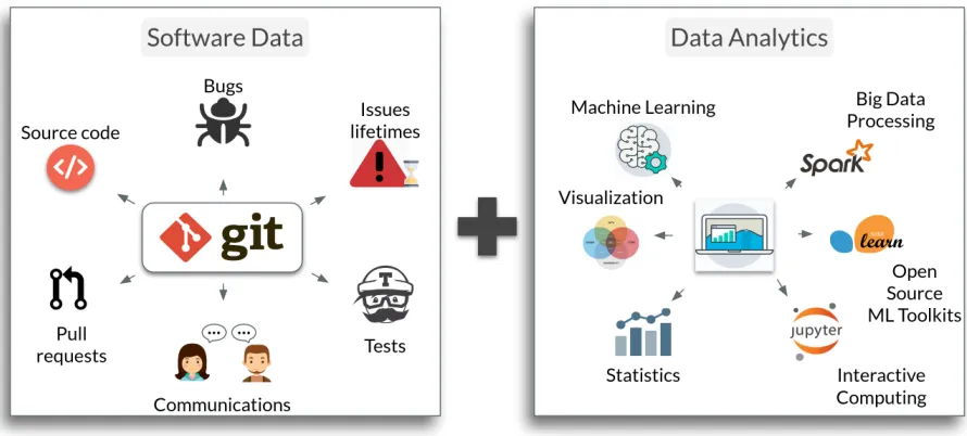
Figure 1.1 Software Analytics . . . 2
Figure 2.1 Bad smells from different sources. Check marks (Ø) denote a bad smell was mentioned. Numbers or symbolic labels (e.g. "VH") denote a priorization comment (and “?” indicates lack of consensus). Empty cells denote some bad smell listed in column one that was not found relevant in other studies. Note: there are many blank cells. . . 14
Figure 2.2 Contradictory conclusions from OO-metrics studies for defect pre-diction. Studies report significant (“+”) or irrelevant (“-”) metrics verified by univariate prediction models. Blank entries indicate that the corresponding metric is not evaluated in that particular study. Colors comment on the most frequent conclusion of each column. CBO=coupling between objects; RFC=response for class (#meth-ods executed by arriving messages); LCOM=lack of cohesion (pairs of methods referencing one instance variable, different definitions of LCOM are aggregated); NOC=number of children (immediate subclasses); WMC=#methods per class. . . 15
Figure 2.3 An example of how developers might use planning to reduce software defects. . . 23
Figure 2.4 Datasets from 4 chosen domains. . . 27
Figure 2.5 Static code metrics used in defects and code smells data sets. . . 28
Figure 2.6 Metrics used in issue lifetimes data. . . 29
Figure 2.7 Metrics used in effort estimation dataset. . . 29
Figure 2.8 A simple example of computing overlap. Here a ‘+’ represents an in-crease, a ‘−’ represents adecrease, and a ‘·’ represents no-change. Columns shaded in blue indicate a match between developer’s change and the recommendation made by a planner. . . 41
Figure 3.1 The Bellwether Framework . . . 56
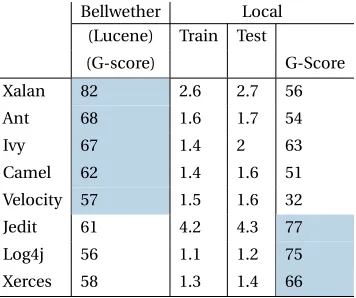
Figure 3.4 Code Smells: This figure compares the prediction performance of the bellwether dataset (xalan,mvnforum) against other datasets (other rows).Bellwether Methodagainst Transfer Learners (columns) for detecting code smells. The numerical value seen here are the median G-scores from Equation 2 over 30 repeats where one dataset is used as a source and others are used as targets in a round-robin fashion. Higher values are better and cells highlighted in gray produce the best Scott-Knott ranks. The last row in each community indicate Win/Tie/Loss(W/T/L). Thebellwether Methodis the overall best. . . 61 Figure 3.5 Issue Lifetime: This figure compares the prediction performance
of the bellwether dataset (qpid) against other datasets (rows) and various transfer learners (columns) for estimating issue lifetime. The numerical value seen here are the median G-scores from Equation 2 over 30 repeats where one dataset is used as a source and others are used as targets in a round-robin fashion. Higher values are better and cells highlighted in gray produce the best Scott-Knott ranks. The last row in each community indicate Win/Tie/Loss(W/T/L). TNB has the overall best Win/Tie/Loss ratio. . . 62 Figure 3.6 Defect Datasets: This figure compares the prediction performance
of the bellwether dataset (Lucene,Zxing,LC) against other datasets (other rows).Bellwether Methodagainst Transfer Learners (columns) for detecting defects. The numerical value seen here are the median G-scores from Equation 2 over 30 repeats where one dataset is used as a source and others are used as targets in a round-robin fashion. Higher values are better and cells highlighted in gray produce the best Scott-Knott ranks. The last row in each community indicate Win/Tie/Loss(W/T/L).TCA+is the overall best transfer learner. . . . 63 Figure 3.7 Effort Estimation: This figure compares the performance of the
bell-wether dataset (cocomo) against other datasets (rows) and Transfer Learners (columns) for estimating effort. The numerical value seen are the median Standardized Accuracy scores from Equation 3 over 40 repeats.Bellwether Methodhas the best Win/Tie/Loss ratio. . . 64 Figure 3.8 Experiments with incremental discovery of bellwethers. Note that
the latest version of lucene (lucene-2.4) has statistically similar per-formance to using the other older versions of lucene. . . 64 Figure 3.9 An example of source instability in defect datasets studied here. The
Figure 4.1 Some configuration options for
SQLite
. . . 81Figure 4.2 BEETLE framework . . . 84
Figure 4.3 Pseudocode forDiscovery . . . 85
Figure 4.4 Pseudocode forTransfer . . . 85
Figure 4.5 A contrived example to illustrate the challenges with MMRE and rank based measures . . . 95
Figure 4.6 Median NAR of 30 repeats. Median NAR is the normalized absolute residual values as described in Equation 4.2, and IQR the difference between 75th percentile and 25th percentile found during multiple repeats. Lines with a dot in the middle ( s), show the median as a round dot within the IQR. All the results are sorted by the median NAR: a lower median value is better. The left-hand column (Rank) ranks the various techniques where lower ranks are better. Overall, we find that there is always at least one environment, denoted in blue , that is much superior (lower NAR) to others. . . 99
Figure 4.7 Win/Loss analysis of learning from the bellwether environment and target environment using Scott Knott. The x-axis represents the percentage of data used to build a model and y-axis is the count. BEETLE wins in all software systems (since BEETLE wins more times than losses) except for SAC– and only when we have measured more that 50% of the data. . . 101
Figure 4.8 Comparison between state-of-the-art transfer learners and BEETLE. The best transfer learner is shaded blue . The “ranks” shown in the left-hand-side column come from the statistical analysis described in §4.2.8.. . . 104
Figure 4.9 BEETLE v/s state-of-the-art transfer learners. The numbers in parenthesis represent the numbers of measurements BEETLE uses in comparison to the state-of-the-art learners. . . 105
Figure 5.1 Relationship of this work to our prior research. Within project trained and tested data miners using data from the same project. Cross projects train on one project, then test on another. Homogeneous learning requires the attribute names to be identical in the training and test set. Heterogeneous learning relaxes that requirement; i.e. the attribute names might change from the training to the test set. . 108
Figure 5.3 To build the decision tree, we find the most informative feature,i.e., the feature which has the lowest mean entropy of splits and construct a decision tree recursively in a top-down fashion as show above. . . . 118 Figure 5.4 For ever test instance, we pass it down the decision tree constructed
in Figure 5.3. The node it lands is called the “start”. Next we find all the “end” nodes in the tree, i.e., those which have the lowest likelihood of defects (labeled in black below). Finally, perform a random-walk to get from “start” to “end”. We use the mined itemsets from Figure 5.2 to guide the walk. When presented with multiple paths, we pick the one which has the largest overlap with the frequent items. e.g., in the below example, we would pick path (b) over path (a). . . 119 Figure 5.5 A simple example of computing overlap. Here a ‘·’ represents
no-change. Columns shaded in gray indicate a match between devel-oper’s changes and planner’s recommendations. . . 124 Figure 5.6 Sample charts to illustrate the format used to present the results. . . 126 Figure 5.7 A count of number of test instances where the developer changes
overlaps a planner recommendation. The overlaps (in the x-axis) are categorized into four ranges for every dataset (these are 0≤Overlap≤
25, 26 ≤ Overlap ≤ 50, 51 ≤ Overlap ≤ 75, and 76 ≤ Overlap ≤
100). For each of the overlap ranges, we count the the number of instances in the validation set where overlap between the planner’s recommendation and the developers changes fell in that range. Note: Higher countsfor larger overlap isbetter, e.g.,C o u n t([75, 100]) > C o u n t([0, 25))is considered better. . . 128 Figure 5.8 A count of total numberdefects reducedas a result each planners’
rec-ommendations. The overlaps are again categorized into four ranges for every dataset (denoted bym i n ≤ O v e r l a p <m a x). For each of the overlap ranges, we count the total number ofdefects reduced and in the validation set for the classes that were defective in the test set as a result of overlap between the planner’s recommendation and the developers changes that fell in the given range . . . 130 Figure 5.9 A count of total numberdefects increasedas a result each planners’
Figure 5.10 A count of total numberdefects reducedanddefects increasedas a re-sult each planners’ recommendations. The overlaps are again catego-rized into four ranges for every dataset (denoted bym i n≤O v e r l a p< m a x). For each of the overlap ranges, we count the total number ofdefects reducedanddefects increasedin the validation set for the classes that were defective in the test set as a result of overlap between the planner’s recommendation and the developers changes that fell in the given range . . . 133 Figure 5.11 A count of total numberdefects reducedwith XTREE and BELLTREE.
Highervalues atLargeroverlaps are better. . . 134 Figure 5.12 A count of total numberdefects reducedwith XTREE and BELLTREE.
CHAPTER
1
INTRODUCTION
Figure 1.1Software Analytics
bugs are most likely[Ost04; Men07c], or how long it will take to develop this code[Tur11; Koc12]. In fact, it is now routine for practitioners to treat every planned feature as an “ex-periment”[Sav16]. In this approach, key performance metrics are carefully monitored and analyzed to judge each proposed feature. Even simple design decisions such as the color of a link are chosen by experiments[LV14]. Large organizations like Microsoft routinely practice data driven policy development where organizational policies are learned from an extensive analysis of large datasets collected from developers[BZ14; The15].
Although software analytics has yielded some very promising results, the current gener-ation of software analytics still has some unique challenges that need to be solved:
1. What is to be done when there is not enough data?When a specific project doesn’t have historical data, how does one go about learning?
3. Where should one transfer lessons from?Given the exponential growth in the number of software projects, which project should one transfer lessons from to achieve the best results?
4. How does one obtain actionable insights?Most modern software analytics tools are mostly prediction algorithms (e.g. support vector machines, naive bayes, logistic regres-sion, etc). How does one go from prediction to decision making?
While the first two challenges have been addressed with the use of sophisticated ma-chine learning techniques such astransfer learning. The last two challenges have yet to be solved. This thesis attempts to offer tools and techniques to help address these challenges.
While there is a lack of historical data for a project, we can use one of many transfer learning techniques. However, given the exponential growth in the number of software projects, there is a major issue ofconclusion instability with transfer learning methods when applied to software engineering. Conclusion instability may be defined as follows:
“The more data we inspect from more projects, the more our conclusions change.”
The problem with conclusion instability is that the lessons transfer from a certain project may no longer hold when new data arrives. Conclusion instability is very unsettling for software project managers struggling to find general policies. In order to support managers, who seek stability in their conclusions, while also allowing new projects to take full benefit of the data from recent projects, in this research we recommend that we must forgo attempts togeneralizefrom all data. We believe that a more achievable goal would be toslowthe pace of conclusion change. The approach proposed in this thesis is to declare one project as the“bellwether”1which should be used to make conclusions about all other projects.
oracle for that community. In the rest of this thesis, we will demonstrate that regardless of the sub-domain of software engineering (code smells detection, effort estimation, defect prediction, or performance optimization), there always exists a bellwether dataset that can be used to train relatively accurate quality prediction models.
1.1
Thesis Statement
"Software quality can be improved by generating effective actionable
an-alytics that are stable despite constant change."
1.2
Thesis Contributions
In summary, the key contributions of this work are:
1. Addressing conclusion instability with bellwethers:We show that depending on the source dataset, there can be large variances in the performance of transfer learner. Fur-ther, we show that different source datasets can lead to different (and often contradicting) conclusions. This thesis demonstrates that these issues can be potentially addressed using the bellwether dataset.
2. Empirical evidence for generality of bellwethers:The more the bellwether effect is explored, the more we learn about its broad applicability. Originally, we explored this just in the context of defect prediction, it has now been shown to work also in:
• Code smells detection (specifically God Class and Feature Envy); • Effort estimation;
• Issue lifetime estimation; • Defect Prediction; and • Configuration optimization.
discovered that the transfer learning literature lacks a simple baseline to compare and contrast the various transfer learners.
To address this, we developed a baseline transfer learner called BEETLE (Bellwether Transfer Learner). To the best of our knowledge, our work was the first to offer a baseline for transfer learning and to undertake a case study of all the state-of-the-art transfer learners and validate their usability in domains other than defect prediction with respect to this baseline. In this thesis, we demonstrate that BEETLE is just as effective as other state-of-the-art algorithms such as:
• Transfer Component Analysis (referred to henceforth as TCA+); • Transfer Naive Bayes (hereafter referred to as TNB)[21];
• Value Cognitive Boosting Learner[22]; • Gaussian Processes Modeling; and • Linear Regression.
4. New kinds of software analytics techniques:Another major component of this research was generating actionable insights in software analytics. In order to do this, we devel-oped a novel algorithm call XTREE. Our results have established that planning is quite successful in producing actions that can reduce the number of defects. We show that actions recommended with XTREE has a significant overlap with the actions actually taken by developers in order to reduce defects.
5. Rich replication packages:For all the experiments reported in this thesis, we have made available several replication packages2 3.
1.3
Publications
1.3.1
Published
[1] Krishna, R. & Menzies, T..“Bellwethers: A Baseline Method For Transfer Learning”. In
IEEE Transactions on Software Engineering, 2018.
[2] Krishna, R., Menzies, T., & Layman, L.“Less is more: Minimizing code reorganization
using XTREE”. In Information and Software Technology, 2017.
[3] Krishna, R., Menzies, T., & Fu, W.“Too much automation? The Bellwether Effect and
its Implications for Transfer Learning.” In Intl. Conference on Automated Software Engineering, 2016.
[4] Krishna, R. & Menzies, T.“Actionable=Cluster+Contrast?”. In Intl. Conference on
Auto-mated Software Engineering Workshop, 2015.
1.3.2
Under Review
[1] Krishna, R. & Menzies, T..“Learning Actionable Analytics from Multiple Software Projects”.
Under review in IEEE Transactions on Software Engineering, 2019.
[2] Nair, V., Krishna, R., Menzies, T., Jamshidi, P.,“BEETLE: Finding Better Software
Config-urations by Borrowing from Old Ones”. Under review in IEEE TSE, 2019.
1.3.3
Other Collaborative Publications
[1] Krishna, R., Yu, Z., Agrawal, A., Dominguez, M., Wolf, D.“The ‘BigSE’ Project: Lessons
[2] Krishna, R., Agrawal, A., Rahman, A., Sobran, A., & Menzies, T.“What is the
Connec-tion Between Issues, Bugs, and Enhancements? (Lessons Learned from 800+Software
Projects)”. In ICSE 2018, SEIP.
[3] Wang, J., Yang, Y., Krishna, R., Menzies, T. & Wang, Q.,“Effective Automated Decision
Support for Managing Crowdtesting”. In Intl. Conference on Foundations of Software Engineering, 2019 (accepted);
[4] Chen, J., Nair, V., Krishna, R., & Menzies, T.“Sampling as a Baseline Optimizer for
Search-based Software Engineering”. In IEEE Transactions on Software Engineering, 2018. [5] Chen, D., Fu, W., Krishna, R., & Menzies, T.“Applications of psychological science for
actionable analytics”. In Intl. Conference on Foundations of Software Engineering, 2018. [6] Agrawal, A., Rahman, A., Krishna, R., Sobran, A. & Menzies, T.“We Don’t Need Another
Hero? The Impact of ‘Heroes’ on Software Development”. In Intl. Conf. Software Engi-neering, 2018 SEIP.
[7] Rahman, A., Agrawal, A., Krishna, R., Sobran, A. & Menzies, T. “Characterizing The
Influence of Continuous Integration. Empirical Results from 250+Open Source and
Proprietary Project”. In Intl. Conference on Foundations of Software Engineering, SWAN 2018.
1.3.4
External Validations
[1] Mensah, S., Keung, J., MacDonell, S. G., Bosu, M. F., & Bennin, K. E. (2018). Investigating
the significance of the Bellwether effect to improve software effort prediction: further empirical study. IEEE Transactions on Reliability, 67(3), 1176-1198.
[2] Mensah, S., Keung, J., MacDonell, S. G., Bosu, M. F., & Bennin, K. E. (2017, July).
Software Quality, Reliability and Security (QRS), 2017 IEEE International Conference on (pp. 340-351). IEEE.
[3] Mensah, S., Keung, J., Bosu, M. F., Bennin, K. E., & Kudjo, P. K. (2017). A Stratification
CHAPTER
2
BACKGROUND
2.1
Transfer Learning
When there is insufficient data to apply data miners to learn defect predictors,transfer learningcan be used to transfer lessons learned from othersourceprojectsS to thetarget projectT.
applications. Turhan’s initial experimental results were also very negative: given data from 10 projects, training onS=9 source projects and testing onT =1 target projects resulted in alarmingly high false positive rates (60% or more).
Subsequent research realized that data had to be carefully sub-sampled and possibly transformed before quality predictors from one source are applied to a target project. That work can be divided two ways:
• Homogeneousvsheterogeneous; • Similarityvsdimensionality transform.
Homogeneous, heterogeneous transfer learning operates on source and target data that contain the same, differentattribute names (respectively). This thesis focuses on homogeneous transfer learning, for the following reason. As discussed in the introduction, we are concerned with an IT manager trying to propose general policies across their IT organization. Organizations are defined by what they do—which is to say that within one organization there is some overlap in task, tools, personnel, and development platforms. This overlap justifies the use of lessons derived from transfer learning.
Hence, all our dataset contain overlapping attributes. In our case these attributes are the metrics gathered for each of the projects. As evidence for this, the datasets explored in this work fall into 4 domains; each domain contains so called “communities” of data sets. Each dataset within a community share the same attributes (see Figure 2.4).
Koc15]doubted that a fixed value ofk was appropriate for all data. That work recursively bi-clustered the source data, then pruned the cluster sub-trees with greatest “variance” (where the “variance” of a sub-tree is the variance of the conclusions in its leaves). This method combined row selection with row pruning (of nearby rows with large variance). Other similarity methods[Zha15]combine domain knowledge with automatic processing: e.g. data is partitioned using engineering judgment before automatic tools cluster the data. To address variations of software metrics between different projects, the original metric values were discretized by rank transformation according to similar degree of context factors.
Similarity approaches uses data in its raw form and as highlighted above, it suffers from instability issues. This prompted research onDimensionality transformmethods. These methods manipulate the raw source data until it matches the target. In the case of defect prediction, a “dimension” was one of the static code attributes of Figure 2.5.
An initial attempt on performing transfer learning withDimensionality transformwas undertaken by Ma et al.[Ma12]with an algorithm called transfer naive Bayes (TNB). This algorithm used information from all of the suitable attributes in the training data. Based on the estimated distribution of the target data, this method transferred the source information to weight instances the training data. The defect prediction model was constructed using these weighted training data.
Nam et al. [Nam13] originally proposed a transform-based method that used TCA based dimensionality rotation, expansion, and contraction to align the source dimensions to the target. They also proposed a new approach called TCA+, which selected suitable normalization options for TCA.
al.[Hal12]indicated that data imbalance may be connected to poor performance. They also suggested more studies should be aware of the need to deal with data imbalance. More importantly, they assert that the performance measures chosen canhidethe impact of imbalanced data on the real performance of classifiers.
An approach proposed by Ryu et al.[Ryu16]showed that using Boosting-SVM combined with class imbalance learner can be used to address skewed datasets. They showed improved performance compared to TNB. More recently, in our previous work[Kri16b], we showed that a very simplistic transfer learner can be developed using the “bellwether" dataset with Random Forest. We reported highly competitive performance scores.
When there are no overlapping attributes (in heterogeneous transfer learning) Nam et al.[NK15]found they could dispense with the optimizer in TCA+by combining feature selec-tion on the source/target following by a Kolmogorov-Smirnov test to find associated subsets of columns. Other researchers take a similar approach, they prefer instead a canonical-correlation analysis (CCA) to find the relationships between variables in the source and target data[Jin15].
Considering all the attempts at transfer learning sampled above, our reading of these literature suggests a surprising lack of consistency in the choice of datasets, learning meth-ods, and statistical measures while reporting results of transfer learning. Further, there was no baseline approach to compare the algorithms against.
2.1.1
Conclusion Instability
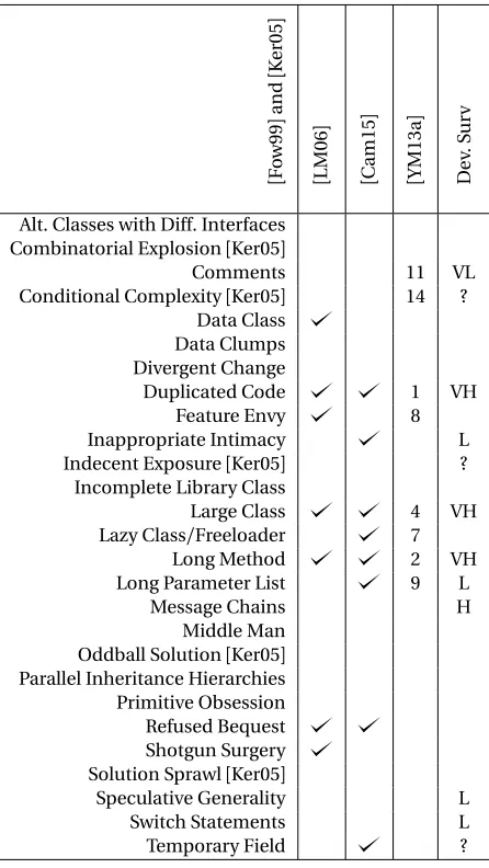
[ F o w99 ] and [ K er05 ] [ LM06 ] [ C am15 ] [ YM13a ] D ev . S ur v
Alt. Classes with Diff. Interfaces Combinatorial Explosion[Ker05]
Comments 11 VL
Conditional Complexity[Ker05] 14 ? Data Class
Data Clumps Divergent Change
Duplicated Code 1 VH
Feature Envy 8
Inappropriate Intimacy L Indecent Exposure[Ker05] ?
Incomplete Library Class
Large Class 4 VH
Lazy Class/Freeloader 7
Long Method 2 VH
Long Parameter List 9 L
Message Chains H
Middle Man Oddball Solution[Ker05] Parallel Inheritance Hierarchies Primitive Obsession Refused Bequest Shotgun Surgery Solution Sprawl[Ker05]
Speculative Generality L
Switch Statements L
Temporary Field ?
Figure 2.1Bad smells from different sources. Check marks ( ) denote a bad smell was mentioned.
Numbers or symbolic labels (e.g. "VH") denote a priorization comment (and “?” indicates lack of consensus). Empty cells denote some bad smell listed in column one that was not found relevant in other studies. Note: there are many blank cells.
ref cbo rfc lcom dit noc wmc #pr
ojects
size
[Ola07] + + + - - + 6 95-201
[Agg09] + + + - - + 12 86 classess (3-12kloc)
[AB06] + + - 1 1700 (110kloc)
[Bas96a] + + - + + + 8 113
[Bri00] + + - + + + 8 114
[Bri01] + + + + - 1 83
[CS00] + + 1 32
[Ema01b] + - 1 42-69
[Ema99] + - - - 1 85
[Tan99] - + - - + 3 92
[Yu02] + + + - + + 1 123 (34kloc)
[SK03] + + + 1 706
[ZL06] + + + - + + 1 145
[Gyi05] + + + + - + 1 3677
[Hol09] + + + + 1 ?
[SL08] + + + + + + 3 ?
[FN01] - + + - - + 8 113
[TM03] + + + + 2 64
[Den03] - - - - 1 3344 modules (2mloc)
[Jan06] + + + - - + 5 395
[Eng09] + + - - + 1 1412
[Sha10a] + + - - + 2 9713
[Sin10] + + - - - + 1 145
[Gla00] + - 1 145
[Ema01a] - - - 1 174
[TV10] - - 0 50
[Xu08] + + - - - + 1 145
[Suc03] + + + 2 294
total+ 18 20 11 11 8 17
total - 4 3 7 14 16 4 KEY: Strong consensus (over 2/3rds)
Total percents: “*” denotes majority conclusion in each column Some consensus (less than 2/3rds)
+ * 64% * 71% * 39% 39% 29% * 61% Weak consensus (about half )
- 14% 11% 25% * 50% * 57% 14% No consensus
Figure 2.2Contradictory conclusions from OO-metrics studies for defect prediction. Studies report
significant (“+”) or irrelevant (“-”) metrics verified by univariate prediction models. Blank entries indicate that the corresponding metric is not evaluated in that particular study. Colors comment on the most frequent conclusion of each column. CBO=coupling between objects; RFC=response for class (#methods executed by arriving messages); LCOM=lack of cohesion (pairs of methods referencing one instance variable, different definitions of LCOM are aggregated); NOC=number of children (immediate subclasses); WMC=#methods per class.
and (b) source instability.
scores are collected from many classifiers which are ranked for tasks such as defect predic-tion[Les08; Hal12; EE08; Men10; Gon08; Rad13; Jia08b; WY13; MK09; Li12; Kho10; Jia09; Gho15; Jia08a; Tan16; Fu16a]. These rankings are then used to identify the “best” defect predictor. However, these prediction tasks assume that future events to be predicted will be near identical to past events. Therefore, given data in the from{xt r a i n,yt r a i n}, prediction
algorithms use this fortrainingin order to form a joint distributionP(X,Y) =P(Y|X)P(Y) and estimate the conditional ˆP(Y|Xt e s t). These predictions will be good as long as the data
is a close approximation of the underlying distribution. As the source of the data changes, the joint distributionP(X,Y)changes to reflect this new data. This gradual change in the underlying distribution of training data with the arrival of new data is calleddata drift. It is widely accepted that thisdriftis the leading cause of instability of prediction models[QC09; Han06; Sto08]. Performance instability can result in large variances in the quality of predic-tions. Numerous researchers[Fu16a; AM17]have shown that changing only the data and retaining the same defect predictor can result in statistically significant differences. (b)Source Instability:This arises due to the constant influx of potential new data sources. In methods such as transfer learning, where we translate quality predictors learned in one data set to another, arrival of new data would require changing models all the time as the transfer learners continually exchange new models to the already existing ones. However, as demonstrated in subsequent parts of this section, each new data source can produce completely different and often contradicting conclusions. Identifying a reliable source of data from all the available options is a pressing issue; more so for methods such as transfer learning since they place an inherent faith in quality the data source. If a change in data source can also change the conclusions, then not being able to identify a reliable data source would limit one from leveraging the full benefits of transfer learning.
engi-neering. The studies explored in the rest this section sample some instances of instability and its prevalence in the domains of software engineering studied here1. Note the vast
contradictions in conclusions in each of these domains.
2.1.1.1 Code Smells
Research on software refactoring endorses the use of code-smells as a guide for improving the quality of code as a preventative maintenance. However, as discussed below, a lot of the research on bad-smells suffers from conclusion instability.
There is much contradictory evidence on whether programmers should take heed of these guidelines or ignore them. For instance, a systematic literature review conducted by Tufano et al.[Tuf15]lists dozens of papers that recommend tools for repair and detection of code smells. On the other hand, several other researchers cast doubt on the value of code smells and their use as triggers for change[Man04; YM13a; Sjo13].
Further, this contradiction is also frequently seen among domain experts. Researchers caution that developers’ cognitive biases can lead to misleading assertions that some things are important when they are not. According to Passos et al.[Pas11], developers often assume that the lessons they learn from a few past projects are general to all their future projects. They comment, “past experiences were taken into account without much consideration for their context”[Pas11]. This warning is echoed by Jørgensen & Gruschke[JG09]. They report that the supposed software engineering experts seldom use lessons from past projects to improve their future reasoning and that such poor past advice can be detrimental to new projects.[JG09].
evidence. Devanbu et al. examined responses from 564 Microsoft software developers from around the world. They comment programmer beliefs can vary with each project, but do not necessarily correspond with actual evidence in that project[Dev16].
The above remarks seem to hold true for bad smells. As shown in Figure 2.1, there is a significant disagreement on which bad smells are important and relevant to a particular project. In that figure, the first column lists commonly mentioned bad smells and comes from Fowler’s 1999 text[Fow99]. The other columns show conclusions from other studies about which bad smells matter most2. From this figure, it is easy to note the lack of con-sensus among developers, text books, and tools. They all disagree on which bad smells are important; just because one developer strongly believes in the importance of a bad smell, it does not mean that the same belief transfers to other developers.
In summary, we seek methods like bellwethers in order to draw stable conclusions. A particular challenge in each of the study in Figure 2.1 is the lack of consistent data source over the period of time these studies were undertaken. In such cases, bellwether datasets can be particularly useful.
2.1.1.2 Defect Prediction
conducted a large scale systematic literature review[Men11a]. We distilled our findings into a list of 28 studies. We noted that they offered contradictory conclusions regarding the effectiveness of OO metrics. These findings are tabulated in Figure 2.2. The figure offers a troubling prospect for managers of a software project. The only concrete finding they can derive from this figure is that response for class is often a useful indicator of defects. Each study makes a clear, but usually different, conclusion regarding the usefulness of other metrics.
In a study of conclusion instability, Turhan [Tur12] showed that the reason for this inconsistency is due to dataset drift. That work reported different kinds of data drift within software engineering data, such as: (1) Source component shift; (2) Domain Shift; (3) Imbal-anced Data, etc. Further, he noted that all contribute significantly to the issue of conclusion instability. In our previous work, we offered further evidence to such a drift by demonstrat-ing that different clusters within the data provided completely different models[Men11a]. Further, the models built from specialized regions within a specific data set sometimes perform better than those learned across all data. However, new data is constantly arriving, and finding these specialized regions with new data turns into an arduous task. In such cases, tools like bellwethers offer a way to draw conclusions from a stable project. As long as the bellwether project remains unchanged so does the conclusions we derive from that project.
2.1.1.3 Effort Estimation
was stable while the variance in dozens of other coefficients were extremely large. In fact, in the case of five coefficients, the values even changed from positive to negative across different samples in a cross-validation study.
Other studies on effort estimation also report very similar findings. Jørgensen[Jor04] compared model-based to expert-based methods in 15 different studies. That study re-ported that: five studies favored expert-based methods, five found no difference, and five favored model-based methods. Similarly, Kitchenham et al.[Kit07a]reviewed seven studies to check the effect of data imported from other organizations as compared with local data for building effort models. Of these seven studies, three found that models from other orga-nizations were not significantly worse than those based on local data, while four found that they were significantly worse. MacDonell and Shepperd[MS07]also performed a review on effort estimation models by replicating Kitchenham et al.[Kit07a]. From a total of 10 studies, two were found to be inconclusive, three supported global models, and five supported local models. Similarly, Mair and Shepperd[MS05]compared regression to analogy methods for effort estimation and found conflicting evidence. From a total of 20 empirical studies, (a) seven recommended regression for building effort estimators; (b) four were indifferent; and (c) nine favored analogy.
2.2
Planning
1. What exactly do you mean by “planning"?
We distinguish planning from prediction for software quality as follows: Quality prediction points to the likelihood of defects. Predictors take the form:
whereincontains many independent features (such as OO metrics) andoutcontains some measure of how many defects are present. For software analytics, the function f is learned via data mining (for static code attributes for instance).
On the other hand, quality planning generates a concrete set of actions that can be taken (as precautionary measures) to significantly reduce the likelihood of defects occurring in the future.
For a formal definition of plans, consider a defective test exampleZ, planners proposes a planD to adjust attributeZj as follows:
∀δj ∈∆:Zj =
Zj+δj ifZj is numeric
δj otherwise
The above plans are described in terms of a range of numeric values. In this case, they represent an increase (or decrease) in some of the static code metrics of Figure 2.5. However, these numeric ranges in and of themselves may not very informative. It would be beneficial to offer a more detailed report on how to go about implementing these plans. For example, to (say) simplify a large bug-prone method, it may be useful to suggest to a developer to reduce its size (e.g., by splitting it across two simpler functions).
2. How to operationalize plans?
However, this data is not accessible. Therefore, we must seek alternative ways to imple-ment plans. One way is to is to use a reverse engineering technique popularized in recent literature. In these techniques, plans, which are in the form of a range numeric range, are mapped into specific actions that will improve the quality of their designs. There has been a number of recent research by the SE community[SS07; DB06; Kat02; BA09], including one of our previous work[Kri17c], that attempt to tackle this very issue. Stroggylos & Spinel-lis[SS07]studied the impact of CK-metrics to assert if performing reorganization was useful in reducing bugs and improving software quality, they reported a strong correlation be-tween these metrics and software quality. Du Bois[DB06]conducted a study that explored coupling and cohesion metrics and reported similar findings. Elish & Alshayeb[EA11; EA12] conducted a systematic study to categorize code reorganization procedures in terms of their measurable effect on software quality attributes. Their studies showed how each reorganization action would impact several of the CK-metrics.
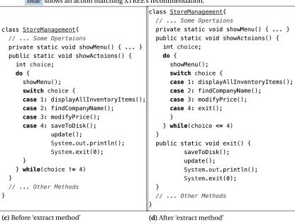
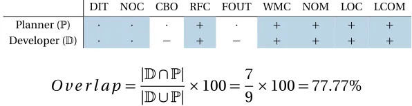
For example, consider Figure 2.3. Let’s say a planner has recommended the changes shown in Figure 2.3(a). Then, we use 2.3(b) to look-up possible actions developers may take, there we see that performing an “extract method” operation may help alleviate certain defects (this is highlighted in blue ). In 2.3(c) we show a simple example of a class where the above operation may be performed. In 2.3(d), we demonstrate how a developer may perform the “extract method”.
3. Why use automatic methods to find quality plans? Why not just use domain knowledge;
e.g. human expert intuition?
DIT NOC CBO RFC FOUT WMC NOM LOC LCOM
· · · 4 · 4 4 4 4
(a)Recommendations from some planner. Here a ‘4’ represents anincrease, a ‘5’ and a ‘·’ representsno-change.
Action DIT NOC CBO RFC FOUT WMC NOM LOC LCOM
Extract Class 4 5 4 5 5 5 5
Extract Method 4 4 4 4 4
Hide Method
Inline Method 5 5 5 5 5
Inline Temp 5
Remove Setting Method 5 5 5 5 5
Replace Assignment 5
Replace Magic Number 4
Consolidate Conditional 4 4 4 5 4
Reverse Conditional
Encapsulate Field 4 4 4 4
Inline Class 5 4 5 4 4 4 4
(b)A sample of possible actions developers can take. Here a ‘4’ represents an
increase, a ‘5’ represents adecrease, and an empty cell representsno-change. Taken from[SS07; DB06; Kat02; BA09; EA11; EA12]. The action highlighted in
blue shows an action matching XTREE’s recommendation.
(c)Before ‘extract method’ (d)After ‘extract method’
all their future projects. They comment, “past experiences were taken into account without much consideration for their context”[34]. Jorgensen and Gruschke[JG09]offer a similar warning. They report that the supposed software engineering “gurus” rarely use lessons from past projects to improve their future reasoning and that such poor past advice can be detrimental to new projects[JG09]. Other studies have shown some widely-held views are now questionable given new evidence. Devanbu et al. examined responses from 564 Microsoft software developers from around the world. They comment programmer beliefs can vary with each project, but do not necessarily correspond with actual evidence in that project[Dev16].
Given the diversity of opinions seen among humans, it seems wise to explore automatic oracles for planning quality improvement change.
2.2.1
Planning in Classical AI
In classical AI, planning usually refers to generating a sequence of actions that enables anagentto achieve a specificgoal[RN95]. In an idealized situation, it is assumed that the possible initial states of the world is known and so are the description of the desired goal in addition to the set of possible and feasible actions. In such a hypothetical situation, planning results in generating a set of actions that is guaranteed to enable one to reach a desired goal. This can be achieved by classical search-based problem solving approaches or logical planning agents. Such planning tasks now play a significant role in a variety of demanding applications, ranging from controlling space vehicles and robots to playing the game of bridge[Gha04].
2.2.1.1 Classical Planning
A simple abstraction of the planning problem is known as classical planning. Classical planning assumes that the initial state is fully-observable and any action is deterministic. Such an assumption enables us to predict the outcome of an action accurately every single time. Further, plans can be defined as sequences of actions, because it is always known in advance which actions will be needed[FN71].
Classical Planning is most useful when the problem is not very complex and the simpli-fying assumptions mentioned above lead to a development of a well-founded model[WJ95]. In the case of complex domains like software engineering, performing a search of plans is highly inefficient. It becomes very difficult to pick the correct search space, algorithm, and heuristics for finding these plans[Gha04].
2.2.1.2 Probabilistic Planning
2.2.1.3 Preference-based Planning
The preference based planning is an extension of the above planning schemes with a focus on producing plans that satisfy as many user-defined constraints (preferences) as possible[SP06]. These preferences as defined by the user are generally not hard constrains, rather they define the quality of the plan, which increases as more of the preferences are satisfied. Algorithms that can solve constraint satisfaction problems are well suited to solve these forms of planning problems. Other popular algorithms include PPLAN[SP06]and HTN[BM09]. However, existence of a model precludes the use of this planning approach. This is a major impediment, since for reasons discussed in the following section, not every domain has a reliable model.
2.3
Target Domains
The rest of this work attempts to discover bellwethers and assesses the performance of bellwethers as baseline transfer learning method. For this, we explore 4 domains in SE: code smells, issue lifetime estimation, effort estimation, and defect prediction.
2.3.1
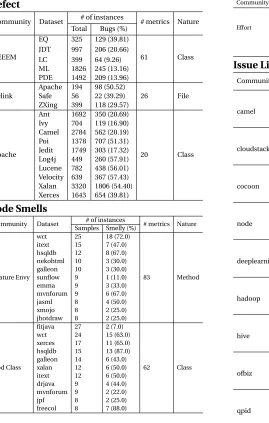
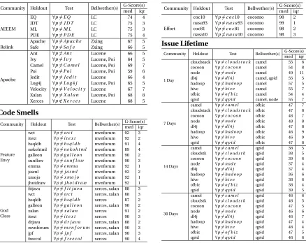
Code Smells
Defect
Community Dataset # of instances # metrics Nature Total Bugs (%)
AEEEM
EQ 325 129 (39.81)
61 Class
JDT 997 206 (20.66) LC 399 64 (9.26) ML 1826 245 (13.16) PDE 1492 209 (13.96)
Relink
Apache 194 98 (50.52)
26 File
Safe 56 22 (39.29) ZXing 399 118 (29.57)
Apache
Ant 1692 350 (20.69)
20 Class
Ivy 704 119 (16.90) Camel 2784 562 (20.19) Poi 1378 707 (51.31) Jedit 1749 303 (17.32) Log4j 449 260 (57.91) Lucene 782 438 (56.01) Velocity 639 367 (57.43) Xalan 3320 1806 (54.40) Xerces 1643 654 (39.81)
Code Smells
Community Dataset # of instances # metrics Nature Samples Smelly (%)
Feature Envy
wct 25 18 (72.0)
83 Method itext 15 7 (47.0)
hsqldb 12 8 (67.0) nekohtml 10 3 (30.0) galleon 10 3 (30.0) sunflow 9 1 (11.0) emma 9 3 (33.0) mvnforum 9 6 (67.0) jasml 8 4 (50.0) xmojo 8 2 (25.0) jhotdraw 8 2 (25.0)
God Class
fitjava 27 2 (7.0)
62 Class wct 24 15 (63.0)
xerces 17 11 (65.0) hsqldb 15 13 (87.0) galleon 14 6 (43.0) xalan 12 6 (50.0) itext 12 6 (50.0) drjava 9 4 (44.0) mvnforum 9 2 (22.0) jpf 8 2 (25.0) freecol 8 7 (88.0)
Effort Estimation
Community Dataset Samples Range (min-max) # metrics
Effort
coc10 95 3.5 - 2673
24 nasa93 93 8.4 - 8211
coc81 63 5.9 - 11400 nasa10 17 320 - 3291.8 cocomo 12 1 - 22
Issue Lifetime
Community Dataset # of instances # metrics Total Closed (%)
camel
1 day
5056
698 (14.0)
18 7 days 437 (9.0) 14 days 148 (3.0) 30 days 167 (3.0)
cloudstack 1 day
1551
658 (42.0)
18 7 days 457 (29.0) 14 days 101 (7.0) 30 days 107 (7.0)
cocoon
1 day
2045
125 (6.0)
18 7 days 92 (4.0) 14 days 32 (2.0) 30 days 45 (2.0)
node
1 day
2045
125 (6.0)
18 7 days 92 (4.0) 14 days 32 (2.0) 30 days 45 (2.0)
deeplearning 1 day
1434
931 (65.0)
18 7 days 214 (15.0) 14 days 76 (5.0) 30 days 72 (5.0)
hadoop
1 day
12191 40 (0.0)
18 7 days 65 (1.0) 14 days 107 (1.0) 30 days 396 (3.0)
hive
1 day
5648
18 (0.0)
18 7 days 22 (0.0) 14 days 58 (1.0) 30 days 178 (3.0)
ofbiz
1 day
6177
1515 (25.0)
18 7 days 1169 (19.0) 14 days 467 (8.0) 30 days 477 (8.0)
qpid
1 day
5475
203 (4.0)
18 7 days 188 (3.0) 14 days 84 (2.0) 30 days 178 (3.0)
Figure 2.4Datasets from 4 chosen domains.
like PMD3, CheckStyle4, FindBugs5, and SonarQube6. Until recently, most detection tools for code smells make use of detection rules based on the computation of a set of metrics, e.g.,
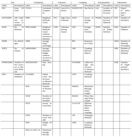
Size Complexity Cohesion Coupling Encapsulation Inheritance Label Description Label Description Label Description Label Description Label Description Label Description LOC Lines Of
Code
CYCLO Cyclomatic Complex-ity
LCOM Lack of Co-hesion
FANOUT/IN Fan Out/In LAA Locality of Attribute Accesses DIT Depth of Inher-itance Tree LOCNAMM LOC
(with-out ac-cessor or mutator) WMC Weighted Methods Count
TCC Tight Class Cohesion
ATFD Access to Foreign Data
NOAM Number of Accessor Methods
NOI Number of Interfaces
NOM No. of
Methods WMCNAMM Weighted Methods Count (without accessor or mutator) CAM Cohesion Among classes FDP Foreign Data Providers NOPA Number of Public Attribute
NOC Number of Children
NOPK No. of Pack-ages
AMW Average
Meth-odsWeight
RFC Response for a Class
NMO Number of Methods Overridden
NOCS No. of
Classes AMWNAMM Average Methods Weight (without accessor or mutator) CBO Coupling Between Objects
NIM Number of Inherited Methods
NOMNAMM Number of Not Acces-sor or Mu-tator Meth-ods
MAXNESTING Max Nest-ing
CFNAMM Called For-eign Not Accessor or Mutator Methods NOII Number of Imple-mented Interfaces
NOA Number of Attributes CLNAMM Called Local Not Accessor or Mutator Methods CINT Coupling Intensity NOP Number of Parame-ters MaMCL Maximum Message Chain Length NOAV Number of
Accessed Variables
MeMCL Mean Mes-sage Chain Length ATLD Access to
Local Data
CA/CE/IC Afferent/ Efferent/ Inher-itance coupling NOLV Number of
Local Vari-able
CM Changing Methods
WOC Weight Of Class
CBM Coupling between Methods MAX_CC/AVG_CC Maximum/
Average McCabe
Figure 2.5Static code metrics used in defects and code smells data sets.
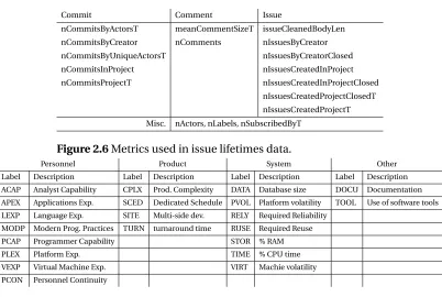
Commit Comment Issue
nCommitsByActorsT meanCommentSizeT issueCleanedBodyLen
nCommitsByCreator nComments nIssuesByCreator
nCommitsByUniqueActorsT nIssuesByCreatorClosed
nCommitsInProject nIssuesCreatedInProject
nCommitsProjectT nIssuesCreatedInProjectClosed
nIssuesCreatedProjectClosedT nIssuesCreatedProjectT Misc. nActors, nLabels, nSubscribedByT
Figure 2.6Metrics used in issue lifetimes data.
Personnel Product System Other
Label Description Label Description Label Description Label Description ACAP Analyst Capability CPLX Prod. Complexity DATA Database size DOCU Documentation APEX Applications Exp. SCED Dedicated Schedule PVOL Platform volatility TOOL Use of software tools LEXP Language Exp. SITE Multi-side dev. RELY Required Reliability
MODP Modern Prog. Practices TURN turnaround time RUSE Required Reuse
PCAP Programmer Capability STOR % RAM
PLEX Platform Exp. TIME % CPU time
VEXP Virtual Machine Exp. VIRT Machie volatility
PCON Personnel Continuity
Figure 2.7Metrics used in effort estimation dataset.
More recently, Fontana et al.[Arc16]in their study of several code smells, considered 74 systems for their analysis and validation. They experimented with 16 different machine learning algorithms. They made available their dataset, which we have adapted for our applications in this study. These datasets were generated using the Qualitas Corpus (QC) of systems[Tem10]. The Qualitas corpus is composed of 111 systems written in Java, char-acterized by different sizes and belonging to different application domains. Fontana et al.[Arc16]selected a subset of 74 systems for their analysis. The authors computed a large set of object-oriented metrics belonging to class, method, package, and project level. A detailed list of metrics and their definitions are available in appendices of[Arc16]. The code smells repository we use comprises of 22 datasets for two different code smells: Feature envy and God Class. The God Class code smell class level code smell that refers to classes that tend to centralize the intelligence of the system. Feature Envy is a method level smell that tends to use many attributes of other classes (considering also attributes accessed through accessor methods).
The number of samples in these datasets are particularly small. For our analysis, we retained only datasets with at least 8 samples so that the transfer learners used here function reliably. This lead us to a total of 22 datasets shown in Figure 2.4.
2.3.2
Issue Lifetime Estimation
stakeholders involved in a software project. Predicting issue lifetime helps software devel-opers better prioritize work; helps managers effectively allocate resources and improve consistency of release cycles; and helps project stakeholders understand changes in project timelines and budgets. It is also useful to be able to predict issue lifetime specifically when the issue is created. An immediate prediction can be used, for example, to auto-categorize the issue or send a notification if it is predicted to be an easy fix.
As an initial attempt, Panjer[Pan07]used logistic regression models to classify bugs as closing in 1.4, 3.4, 7.5, 19.5, 52.5, and 156 days, and greater than 156 days. He was able to achieve an accuracy of 34.9%. Giger et al.[Gig10]used models constructed with decision trees to predict for issue lifetimes in Eclipse, Gnome, and Mozilla. They were able obtain a peak precision of 65% by dividing time into 1, 3, 7, 14, 30 days. Zhang et al.[Zha13]developed a comprehensive system to predict lifetime of issues. They used a Markov model with a kNN-based classifier to perform their prediction. More recently, Rees-Jones et al[Rj17] showed that using Hall’s CFS feature selector and C4.5 decision tree learner a very reliable prediction of issue lifetime could be made.
Figure 2.4 shows a list of 8 projects used to study issue lifetimes. These projects were selected by our industrial partners since they use, or extend, software from these projects. It forms a part of an ongoing study on prediction of issue lifetime by Rees-Jones et al.[Rj17]. The authors note that one issue in preparing their data was a small number ofstickyissues. They define sticky issues as one which was not yet closed at the time of data collection. As recommended by Rees-Jones et al.[Rj17], we removed these sticky issues from our datasets.
2.3.3
Effort Estimation
The nature of effort estimation and the corresponding data is unlike that of other domains. Firstly, while domains like defect prediction datasets often store several thousand samples of defective and non-defective samples, effort data is usually smaller with only a few dozen samples at most. Secondly, unlike defect dataset or code smells, effort is measured using, sayman-hours, which is a continuous variable. These differences requires us to significantly modify existing transfer learning techniques to accommodate this kind of data.
Transfer learning attempts have been made in defect prediction before albeit with limited success. Kitchenham et al.[Kit07b]reviewed 7 published transfer studies in effort estimation. They found that in most cases, transferred data generated worse predictors than using within-project information. Similarly, Ye et al.[Yan11]report that the tunings to Boehm’s COCOMO model have changed radically for new data collected in the period 2000 to 2009. Kocaguneli et al.[Koc15]used analogy-based effort estimation with relevancy filtering using a method called TEAK for studying transfer learning in effort estimation. He found that it outperforms other approaches such as linear regression, neural networks, and traditional analogy-based reasoners. Since then, however, newer more sophisticated transfer learners have been introduced. Krishna et al.[Kri16b]suggest that relevancy fil-tering (for defect prediction tasks) would never have been necessary in the first place if researchers had instead hunted for bellwethers. Therefore, in this work, we revisit transfer learning in effort estimation keeping in mind these changing trends.
show that this model works better than (or just as well as) other models they’ve previously studied. We use 5 datasets shown in Figure 2.4. Here, COC81 is the original data from 1981 COCOMO book[Boe81b]. This comes from projects dated from 1970 to 1980. NASA93 is NASA data collected in the early 1990s about software that supported the planning activities for the International Space Station. The other datasets are NASA10 and COC05 (the latter is proprietary and cannot be released to the research community). The non-proprietary data (COC81 and NASA93 and NASA10) are available at http://tiny.cc/07wvjy.
2.3.4
Defect Prediction
to defect prediction techniques. These techniques enable developers to target defect-prone areas faster, but do not guide developers toward a particular fix. The defect prediction models are easier to use in that sense that they prioritizebothcode review and testing resources (these areas complement each other).
Moreover, defect predictors often find the location of 70% (or more) of the defects in code[Men07a]. Defect predictors have some level of generality: predictors learned at NASA[Men07a]have also been found useful elsewhere (e.g. in Turkey[Tos10; Tos09]). The success of this method in predictors in finding bugs is markedly higher than other currently-used industrial methods such as manual code reviews. For example, a panel atIEEE Metrics 2002[Shu02]concluded that manual software reviews can find≈60% of defects. In another work, Raffo documents the typical defect detection capability of industrial review methods: around 50% for full Fagan inspections[Fag76]to 21% for less-structured inspections.
Not only do static code defect predictors perform well compared to manual methods, they also are competitive with certain automatic methods. A recent study at ICSE’14, Rah-man et al.[Rah14]compared (a) static code analysis tools FindBugs, Jlint, and Pmd and (b) static code defect predictors (which they called “statistical defect prediction”) built using logistic regression. They found no significant differences in the cost-effectiveness of these approaches. Given this equivalence, it is significant to note that static code defect prediction can be quickly adapted to new languages by building lightweight parsers that find information like Figure 2.5. The same is not true for static code analyzers– these need extensive modification before they can be used on new languages.
attributes to decide which modules are worth manual inspections.
The defect dataset we have used come from 18 projects grouped into 3 communities taken from previous transfer learning studies. The projects measure defects at various levels of granularity ranging from function-level to file-level. Figure 2.4 summarizes all the communities of datasets used in our experiments.
For the reasons discussed in §2.1, we explore homogeneous transfer learning using the attributes shared by a community. That is, this study explores intra-community transfer learning and not cross-community heterogeneous transfer learning.
The first dataset, AEEEM, was used by[NK15]. This dataset was gathered by D’Amborse et al.[D’A12], it contains 61 metrics: 17 object-oriented metrics, 5 previous-defect metrics, 5 entropy metrics measuring code change, and 17 churn-of-source code metrics.
The RELINK community data was obtained from work by Wu et al.[Wu11]who used the Understand tool7, to measure 26 metrics that calculate code complexity in order to
improve the quality of defect prediction. This data is particularly interesting because the defect information in it has been manually verified and corrected. It has been widely used in defect prediction[NK15][Wu11][Bas96b][OA96][Kim11].
In addition to this, we explored two other communities of datasets from the SEACRAFT repository8. The group of data contains defect measures from several Apache projects. It
was gathered by Jureczko et al.[JM10]. This dataset contains records the number of known defects for each class using a post-release bug tracking system. The classes are described in terms of 20 OO metrics, including CK metrics and McCabes complexity metrics. Each dataset in the Apache community has several versions. There are a total of 38 different datasets. For more information on this dataset see[Kri16a].
2.4
Evaluation
2.4.1
Evaluating Transfer Learners
2.4.1.1 Evaluation for Continuous Classes
For the effort estimation data in Figure 2.4, the dependent attribute is development effort, measured in terms of calendar hours (at 152 hours per month, including development and management hours). For this, we use general machine learning algorithms as a regressor instead of a classifier.
To evaluate the quality of the learners used for regression, we make use of Standardized Accuracy (SA). The use of SA has been endorsed by several researchers in SE[SM12a; Lan16] Standard Accuracy is computed as below:
S A=1− M AR
2
n2 Pn
i=1
Pj<i
j=1|yi−yj|
×100 (2.1)
Where, MAR is the mean of the absolute error for the predictor of interest. E.g. for software project estimation, the average of the absolute difference between the effort predicted and the actual effort the project took.
Higher values of SA are considered to bebetter. Note: Some researchers have endorsed the use other metrics such as MMRE to measure the quality of regressor in effort estimation. We have made available a replication package9 with this and other metrics. Interested
2.4.1.2 Evaluation for Discrete Classes
In the context of discrete classes, we define positive and negative classes. With defects, instances with one or more defects are considered to belong to the “positive class” and non-defective instances are considered to belong to the “negative class”. Similarly in code smell detection (smelly samples belong to “positive class”) and in issue lifetime estimation (closed issues belong to “positive class”). Prediction models are not ideal, they therefore need to be evaluated in terms of statistical performance measures.
For classification problems we construct a confusion matrix, with this we can obtain sev-eral performance measures such as: (1)Accuracy: Percentage of correctly classified classes (both positive and negative); (2)Recall or pd: percentage of the target classes (defective instances) predicted. The higher the pd the better ; (3)False alarm or pf: percentage of non-defective instances wrongly identified as defective. Unlike pd, lower the pf implies better quality; (4)Precision: probability of predicted defects being actually defective. Either a smaller number of correctly predicted faulty modules or a larger number of erroneously predicted defect-free modules would result in a low precision.
variables in the datasets commonly studied here. For instance, consider the datasets studied in this work shown in Figure 2.4. There, a number of datasets have highly skewed samples. In these cases, several researchers caution against use of common performance metrics such as precision or F-measure. Menzies et al.[Men07c]in their 2007 paper showed the negative impact of using these metrics. They caution researchers against the use precision when assessing their detectors. They recommend other more stable measures especially for highly skewed data sets. This concern is echoed by several other researchers in SE[Cha03; KM97; Sha10c]. Kubat & Matwin found that the effect of the negative classes (in our context this refers to bug-free/smell-free/closed issues) has a profound impact on the outcome of these metrics. As a remedy, these authors recommend a new evaluation scheme that combines reliable metrics such as recall (p d) and false-alarm (p f).
One such approach that can combine these metrics is to build aReceiver Operating Characteristic (ROC)curve. ROC curve is a plot of Recall versus False Alarm pairing for various predictor cut-off values ranging from 0 to 1. The best possible predictor is the one with an ROC curve that rises as steeply as possible and plateaus at pd=1. Ideally, for each curve, we can measure theArea Under Curve (AUC), to identify the best training dataset. Unfortunately, building an ROC is not straight forward in our case. We have used Random Forest for predicting defects owing to it’s superior performance over several other predic-tors[Les08]. Note that Random Forest lacks a threshold parameter, since this threshold parameter is required in order to generate a set of points to plot the ROC curve, Random Forest is not capable of producing an ROC curve, instead we produce just one point on the ROC curve. It is therefore not possible to compute AUC.
Several authors[Men07c; Sha10c]have previously shown that such a measure is justifiably better than other measures when the test samples have imbalanced distribution in terms of classes. G-Score can by computed by measuring the mean (geometric/harmonic) between the Probability of True Positives (Pd) and Probability of true negatives (1-Pf ). The choice of using geometric mean or harmonic mean depends on the variance in Pd/Pf values. Mathematically, it is known that in cases where samples tend to take extreme values (such as Pd=0 or Pf=1) harmonic mean provides estimates that are much more stable and also more conservative in it’s estimate compared to geometric mean[Xia99]. Therefore, we propose the use of G-Score, measured as follows:
G =2×P d×(1−P f)
1+P d−P f (2.2)
In this work, for the sake of consistency with other SE literature, we report the measures of Pd and Pf reported in terms of the G-Score. Also, note that with the formulation in Equation 2.2,largerG-scores are better.
2.4.2
Evaluating Planners
It can be somewhat difficult to judge the effects of applying plans to software projects. These plans cannot be assessed just by a rerun of the test suite for three reasons: (1) The defects were recorded by a post release bug tracking system. It is entirely possible it escaped detection by the existing test suite; (2) Rewriting test cases to enable coverage of all possible scenarios presents a significant challenge; and (3) It may take a significant amount of effort to write new test cases that identify these changes as they are made.
separately from the primary oracle. This oracles assesses how defective the code is before and after some code changes. For their oracle, Cheng, O’Keefe, Moghadam and Mkaouer et al. use the QMOOD quality model[BD02].
A shortcoming of QMOOD is that quality models learned from other projects may perform poorly when applied to new projects[Men13]. Hence, we eschew older quality models like QMOOD and propose a verification oracle based on theoverlap. between two sets: (1) The changes that developers made, perhaps in response to the issues raised in a post-release issue tracking system; and (2) Plans recommended by an automated planning tool such as XTREE/BELLTREE. Using these two sources of changes, it is possible to compute the extent to which a developer’s action matches that of the actions recommended by planners. This is measured usingoverlap:
Overlap=|D∩P|
|D∪P|×100 (2.3)
That is, we measure overlap using the size of the intersections divided by the size of the union of thechanges. HereDrepresents the changes made by thedevelopersandP
repre-sents the changes recommended by theplanner. Accordingly, the larger the intersection between the changes made by the developers to the changes recommended by the planner, the greater the overlap.