| INVESTIGATION
Statistical Methods for Latent Class Quantitative Trait
Loci Mapping
Shuyun Ye,* Rhonda Bacher,* Mark P. Keller,†Alan D. Attie,†and Christina Kendziorski‡,1 *Department of Statistics,†Department of Biochemistry, and‡Department of Biostatistics and Medical Informatics, University of Wisconsin, Madison, Wisconsin 53706
ABSTRACT Identifying the genetic basis of complex traits is an important problem with the potential to impact a broad range of biological endeavors. A number of effective statistical methods are available for quantitative trait loci (QTL) mapping that allow for the efficient identification of multiple, potentially interacting, loci under a variety of experimental conditions. Although proven useful in hundreds of studies, the majority of these methods assumes a single model common to each subject, which may reduce power and accuracy when genetically distinct subclasses exist. To address this, we have developed an approach to enable latent class QTL mapping. The approach combines latent class regression with stepwise variable selection and traditional QTL mapping to estimate the number of subclasses in a population, and to identify the genetic model that best describes each subclass. Simulations demonstrate good performance of the method when latent classes are present as well as when they are not, with accurate estimation of QTL. Application of the method to case studies of obesity and diabetes in mouse gives insight into the genetic basis of related complex traits.
KEYWORDSQTL mapping; obesity; type II diabetes; latent class regression; stepwise regression; complex traits
I
DENTIFYING the genetic loci underlying a complex trait is a challenging problem that has received considerable at-tention, with robust statistical methods and software now available for identifying multiple, potentially interacting quantitative trait loci (QTL). Broman (2001) and Mackayet al.(2009) provide comprehensive reviews. Although useful, traditional methods assume a single genetic model common to all subjects. This assumption is often violated in practice, for example, when subpopulations having traits governed by dis-tinct genetic models are present. When the assumption of a single model common to all subjects is violated, methods that rely on it may fail to identify important loci.
The idea of subpopulations governed by distinct genetic models is a common one, and, in the simplest of cases, standard methods apply. For example, a phenotype governed by two genetic models, one for males and one for females (i.e., sex defines the subpopulation), can be well represented by a
linear model with an interaction term. A similar example applies to subpopulations governed by genotype at a marker. For example, suppose, in a backcross, quantitative trait y
follows the model y¼mþa1x1þa2x2þbx1x2þe; where
x1andx2represent genotypes at two markers (homozygotes
and heterozygotes with levels 0 and 1, respectively), andeis the Gaussian error term. The model can be rewritten as:
y¼mþa1x1þe1; x2 ¼ 0
y¼ ðmþa2Þ þ ða1þbÞx1þe2; x2 ¼ 1
Here, for subpopulations defined by different levels ofx2;x1
has a different effect ony, as the coefficients ofx1in the two
models differ from each other.
This work concerns the case where subpopulations, re-ferred to hereinafter as classes, are not defined by a known covariate (such as sex, age, marker genotype, etc.), but rather by factors that are unknowna priori. Specifically, we
devel-oped a model-based approach to facilitate QTL mapping in experimental crosses, allowing for the possibility that there may be two latent classes of subjects within a cross, each with its own genetic model affecting a trait. The approach allows a user to estimate the likelihood that two classes of subjects are present, and to estimate the genetic model within each class. Simulations suggest improvements in power when multiple classes are present, with a modest decline in operating Copyright © 2017 by the Genetics Society of America
doi:https://doi.org/10.1534/genetics.117.203885
Manuscript received May 17, 2017; accepted for publication May 18, 2017; published Early Online May 23, 2017.
Available freely online through the author-supported open access option.
Supplemental material is available online athttp://www.genetics.org/lookup/suppl/ doi:10.1534/genetics.117.203885/-/DC1.
characteristics relative to standard approaches when they are not. Further advantages are demonstrated in case studies of obesity and diabetes in mouse.
Materials and Methods details the so-called latent class QTL mapping method (lcQTL), which combines traditional QTL mapping methods with latent class regression. Simula-tion studies to evaluate the operating characteristics of lcQTL compared to traditional QTL mapping approaches are given in the sections Simulated dataand Evaluation of operating characteristics. An application of lcQTL to two obesity and diabetes case studies shows that many obesity and diabetes related clinical traits have two QTL classes, with novel QTL discovered in some cases. An analysis of genome-wide ex-pression data from the same subjects provides insights into class separation (Results).
Methods
Latent class regression
Latent class regression (LCR) methods have been developed to estimate a regression model in the presence of subclasses when predictors are known but subclasses are not. Whereas traditional regression assumes that the relationship between predictors and a response can be described using one model, LCR accommodates the situation in which the relationship changes across latent classes. Specifically, the LCR model (Wedel and DeSarbo 1995), with afixed number ofK com-ponents, assumesKdifferent classes in the data defined by
the relationship between a responseyandppredictor(s)xi; i¼1;. . .;p: Within each class, the relationship between y
andxiis described by a linear model with a Gaussian error term. In different classes, thexi9s have different effects ony, and thus the coefficients (bik;i¼1;. . .;p;k¼1;. . .;K) are different between different classes. For fixed K, the
coeffi-cients of the linear model and error term variance are esti-mated via the expectation-maximization (EM) algorithm (Dempsteret al.1977). Once the parameters are obtained, the optimal number of classes is estimated using an informa-tion criterion such as the Bayesian informainforma-tion criterion (BIC) (Schwarz 1978). Fiara and Soromenho (2010) provide further details, and a literature review of LCR.
Stepwise latent class QTL mapping (lcQTL)
lcQTL mapping: To enable lcQTL mapping, we combine
traditional QTL mapping methods with LCR and stepwise
regression. In short, given a quantitative traityand genotype data on an experimental cross, candidate markers are se-lected. Stepwise regression is then performed for a one-class model and two-class model separately. To compare thefitted models, an information criterion specific to lcQTL mapping is developed. Details of each step follow.
Candidate marker selection:We define a generalized LOD
(gLOD) score for akclass QTL modelgkas follows:
gLODðgkÞ ¼log10
P ðdatajgkÞ
P ðdatajnull modelÞ
wheregkrepresents ak-class LCR model, and the null model contains no QTL. For the one-class model, a standard LOD score profile is calculated via simple marker regression; for the two-class model, a gLOD profile is calculated forK¼2 using LCR one marker at a time. Candidate markers in the one (two) class model are selected as those having high LOD (gLOD) scores, using the marker selection method described in Wanget al.(2011).
Model estimation:For the one-class model, forward regres-sion is conducted using the candidate markers identified until the number of QTL reaches a user-defined maximum; back-ward elimination is then conducted. In both forback-ward and backward elimination, markers are added or deleted based on the BIC; and relevant covariates (age, sex, etc.) are in-cluded. The user-defined maximum is varied within a range to generate a number of candidate models. A penalized gLOD score, p-gLOD, is developed to select a model from the candidate models. As with the penalized LOD score (pLOD) developed by Manichaikul et al. (2009), p-gLOD penalizes the number of QTL in the model, but p-gLOD also penalizes each QTL by significance level, which improves power and FDR. Specifically, p-gLOD is defined as:
p2gLODa ðgÞ ¼gLOD ðgÞ 2l*
XS
j¼1
Ta2Tdiffa;j
wherejindexes markers in the model;Tais a genome-wide gLOD score significance threshold;Tdiff
a;j is the difference be-tween the gLOD score of the jth marker and Ta;andlis a coefficient that determines the penalty strength.Tais chosen as the 1–a quantile of the genome-wide maximum gLOD scores under the null hypothesis of no QTL, derived from permutations; and lis estimated via simulations. The pro-cedure is repeated for two-class model estimation.
Table 1 Simulation set up
Simulation #Classes
Range of % Variance Explained in Class 1
Range of % Variance Explained in Class 2
Range of % Variance Explained Assuming One Class Model
Ia 2 (30, 50) (30, 50) (10, 20)
Ib 2 (30, 50) (30, 50) (10, 20)
Ic 2 (30, 50) (30, 50) (10, 20)
II 1 — — (10, 20)
III 1 — — 0
Evaluation of evidence for multiple classes:In standard LCR, BIC is the most common criteria used to determined the number of classes in the population (Magidson and Vermunt 2004). However, in complex trait mapping, the percentage of variance explained by QTL is relatively low, in which case the BIC lacks power for detecting the existence of latent classes (Tofighi and Enders 2008; Tueller and Lubke 2010). To address this, we use AICc(Hurvich and Tsai 1989) for evaluating evidence of multiple classes. For a model withnobservations andpfree parameters, AICcis defined as follows:
AICc¼AICþ2pðpþ1Þ
n2p21
where AIC is22 *LLþ2p;withLLindicating the log likeli-hood of the model. AICcddenotes the difference between the one- and two-class models. Here, AICcd = 2 and AICcd = 6 are considered as moderate and strong evidence of model differences, as in Kass and Raftery (1995).
Detecting factors associated with classes: As noted above, relevant covariates are adjusted for when estimating the best one- or two-class models. If, after adjusting for obvious cova-riates, there is strong evidence in favor of a two-class model, it may be of interest to identify additional factors associated with the classes. Interactions among markers not considered in the initial model, as well as other covariates such as expression probes or clinical variables, are all possible factors that may be at least in part driving differences between the classes. To evaluate possible factors, we conduct association tests. A subject is assigned into the class having highest posterior probability estimated through the EM algorithm. For factor variables,x2test statistics are calculated, while, for numeri-cal variables, Student’s t-test statistics are used. Each test requires assignment of subjects into classes, and a number of methods could be used. Here, we assign a subject into the class having highest posterior probability as is common in LCR (Fraley and Raftery 2002; Leisch 2004). The topNfactors (those with strongest associations) are considered candidates in
a forward-backward regression, with each candidate factor evaluated using AICcd:The factors included in the model after this stepwise regression are considered factors asso-ciated with the classification if, when factors are included in the model, there is strong evidence of the one-class over the two-class model as assessed via AICc. The idea is that, once the main factors driving class separation are all in-cluded in the model, the one-class model should be sufficient.
Software implementation
All analyses were carried out using R version 3.2.2. For comparisons, we considered scanone (Broman 2003) and
stepwiseqtl(Manichaikulet al.2009) in R/qtl version 1.37– 11, and Wang’s multiple-QTL mapping method version 1.1.3.3 Wanget al.(2011) in R. Each approach was applied using default settings as described in the respective vi-gnettes. Briefly, forscanone, we assume the normal model, and use the EM algorithm to estimate the parameters. For
stepwiseqtl, we assume the normal model, and use multiple imputation as described in Sen and Churchill (2001). For Wang’s multiple-QTL mapping methods, we use BIC(2) as the penalty function. In each step of the stepwise regression detailed in Model estimation, we use the EM algorithm implemented in the Rflexmixpackage (Leisch 2004) version 2.3.13 for parameter estimation. The EM in flexmixis ini-tialized using a random assignment of observations to mix-ture components (Grun and Leisch 2007), and we used this default setting in our application. The hard assignment method inflexmix;also known as maximizing the
classifica-tion likelihood (Fraley and Raftery 2002), was used for membership assignment. This approach assigns a subject into the class with highest posterior probability. Running lcQTL on a clinical trait with sample size of 500 and 2000 markers takes 30–45 min on an Intel Xeon E5645 with 2.40 GHz and 128 GB of RAM, depending on EM convergence time. Note that this does not include the computation time for permutations to determine Ta; the genome-wide gLOD score significance threshold.
Evaluation
When evaluating results, we used 7.5 cM windows (67.5 cM on each side of the true QTL position) to determine whether each detected QTL is a true or false positive. These and other operating characteristics were defined as follows. True Posi-tive: a detected QTL is within the 15 cM window. False Pos-itive: a detected QTL is not within the 15 cM window.False Negative: a true (simulated) QTL is not detected. Power: (# of True Positive QTL)/(# of true QTL). FPR: (# of False Positive QTL)/(# of QTL being considered – # of true QTL). Percentage of variance explained: 12ðSSresÞ=ðSStotÞ;
where: SSres¼
Pn
i¼1ðyi2ybiÞ2 and SStot¼
Pn
i¼1ðyi2yÞ2; wherei¼1;2;. . .;nindexesnsubjects, andyiindexes phe-notype for the ith subject. y is the mean value of
yi;i¼1;. . .;n;and^yiis thefitted value ofyi:For traditional QTL mapping methods, and for lcQTL when there is only one class estimated,^yiis thefitted value calculated from the es-timated QTL model. For lcQTL when there are two classes estimated,^yiis calculated as^yi¼
P2
k¼1Tik^yik;wherekis the index of classes, Tik is the posterior probability of subjecti belonging to classkfrom EM algorithm, and^yikis thefitted value of y for the ithsubject assuming the QTL model of
classk.
Data
Simulated data: Three different sets of simulations were
generated to evaluate the performance of the lcQTL mapping method. The number of classes in the data (one or two), as well as the extent of overlap among QTL in the two-class models, were varied across simulations as described below. In each simulation, the genotype data were taken from an F2 intercross between C57BL/6 (B6) and BTBR mice with 519 mice genotyped at 2057 markers (described in detail in
Case study data); 500 of the 519 mice, and 3 of the 2057 markers (denoted asx1;x2;andx3) were chosen at random
(some 1, 33.82 cM; chromo(some 3, 69.63 cM; and chromo-some 5, 57.05 cM). For each set of simulations, parameters, error terms, and effect sizes were chosen to match features observed in the F2 intercross (see Supplemental Material,File S1for details).
We simulate data in two classes (Simulation I), one class (Simulation II), and noise only (Simulation III) to mimic real data. In each simulation, the parameters (effect size and variance of error term) are chosen so that the percentage of variance explained in each class (when there are two clas-ses), and in the whole dataset matches real data. See Table 1 for details. In Simulation I, the two classes are unbalanced in
size (200 samples in class 1, 300 samples in class 2) as un-balanced class size is common in applications. Simulation Ia, Ib, and Ic have different extents of overlapping QTL. In Sim-ulation Ia and Ib, for the overlapping QTL of the two classes, their effect size in one of the classes is.2 times the effect size in the other class to distinguish the class difference. Specifics on effect sizes (reported as percentage of variance explained) are given in Table 1. In each simulation, the percentage of variance explained in each class and overall is controlled within the range indicated.
In the simulations Ia, Ib, and Ic, the first class has 200 subjects, and the second has 300 subjects. In simula-tion Ia (full overlap), all three QTL, x1;x2;andx3 are
pre-sent in each class, with different effect sizes between classes (the effect size for each marker is more than twice as big in one class than the other). In Simulation Ib (partial over-lap), thefirst class has QTLx1andx2;and the second class
has QTL x2 andx3: Simulation Ic has no overlap among
QTL. Specifically, thefirst class has QTLx1andx2;and the
second class has QTL x3:Simulation II consists of a
one-class model with 500 subjects and three QTL; Simulation III is noise only.
Case study data
We consider two case studies. Thefirst is a backcross from a study of obesity (Reifsnyderet al.2000) containing 204 male mice each genotyped at 85 markers. The mice are generated by crossing the obese, diabetes-prone NZO strain to the rel-atively lean NON strain, and then backcrossing the obese F1 mice to the NON strain. This study measured 24 phenotypes closely related to obesity including body weight, glucose, and insulin level for multiple weeks, and fat pad weights. The second dataset considered is an F2 intercross (C57BL/6 (B6) 3 BTBR) from a study of diabetes in mouse (Wang
et al.2011; Tuet al.2012) with 519 mice (244 females and 275 males). Each mouse is genotyped at 2057 markers and phenotyped for 128 diabetes-related clinical phenotypes in-cluding body weight, insulin level, urinary sodium, and monocyte chemoattractant protein-1 (MCP-1). In addition, mRNA expression traits are available for 40,572 transcripts profiled in islet.
Data availability
The authors state that all data necessary for confirming the conclusions presented in the article are represented fully within the article.
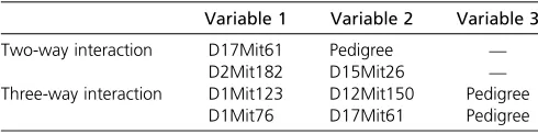
Table 2 Interactions detected by Reifsnyder et al. (2000) for plasma glucose at 20 weeks
Variable 1 Variable 2 Variable 3
Two-way interaction D17Mit61 Pedigree —
D2Mit182 D15Mit26 —
Three-way interaction D1Mit123 D12Mit150 Pedigree D1Mit76 D17Mit61 Pedigree
Table 3 Interactions associated with classes identified by lcQTL for plasma glucose at 20 weeks in the mouse backcross of Reifsnyder
et al.(2000)
Variable 1 Variable 2 Variable 3 Overlap
Two-way interaction D1Mit213 Pedigree — Partial
D6Mit58 Pedigree — New
Three-way Interaction D5Mit7 D17Mit61 Pedigree Partial
Results
Evaluation of operating characteristics
Simulation studies were conducted to investigate the operat-ing characteristics of lcQTL, and to assess how lcQTL compares with competing approaches. Specifically, we considered lcQTL, traditional QTL mapping as implemented inscanone
(Broman 2003) in R/qtl,stepwiseqtl(Manichaikulet al.2009) in R/qtl, and Wang’s multiple-QTL mapping method Wang
et al.(2011). Details on each version and settings are given in Supplemental Section 1. Figure 1 shows the percentage of times the correct number of classes was identified by lcQTL, power, and false positive rates averaged over each set of simulations. Additional rates are provided in Table S1 in
File S1.
Figure 1 demonstrates that lcQTL is able to detect the correct number of classes when latent classes are present (simulations Ia, Ib, and Ic) as well as when they are not (simulations II and III). Also, when latent classes are pre-sent, lcQTL has higher power and reduced false identifica-tions relative to traditional QTL mapping methods. The biggest advantage is observed when there are two classes that do not share all QTL, as in simulations Ib and Ic. In addition, when latent classes are not present, the power and FPR of lcQTL is comparable to traditional methods.
In addition to simulation studies, to evaluate the perfor-mance of lcQTL we consider the phenotype urinary protein from the F2 mouse study, described inCase study data, since this phenotype is known to have a strong sex effect. As detailed in Methods (lcQTL mapping), the lcQTL approach
assumes that standard covariates such as sex are adjusted for in the model, and so any latent classes identified should not be due to differences in these standard covariates. The lcQTL approach did not identify urinary protein as having latent classes. However, as a test of lcQTL, wefit the model without including sex. If lcQTL is effective, it should identify two classes for urinary protein when sex is not included in the original model. We found this to be the case, with lcQTL finding strong evidence of two classes (AICcd¼101:663).
To test the procedure described in lcQTL mapping for identifying factors associated with class membership, we evaluated associations for sex, 40,572 expression probes, and two-way interactions between markers and sex as can-didate factors. The topN¼50 associations were used in sub-sequent stepwise regressions. Of these, sex, interactions between sex and two markers (Chr1.33 and Chr13.24 cM), and the expression probe associated with Kdm6a (a gene on chromosome X), were the factors that were identified as driv-ing the two classes. This proof-of-principle test demonstrates that lcQTL is effective at identifying meaningful subclasses, and in detecting factors associated with distinctions between the classes.
As a second proof-of-principle evaluation, we consider the phenotype plasma glucose at 20 weeks from Reifsnyderet al.
(2000). Clearly, with real data, the true underlying model can only be estimated, not known. However, plasma glucose at 20 weeks was analyzed extensively by Reifsnyder et al.
(2000) using both statistical and visual analyses, and so we consider the model derived in that work as a standard to which we compare results from lcQTL. The model identified
Figure 2 Percentage of variance explained for the 12 clinical traits iden-tified as having two classes via lcQTL in the mouse backcross of Reifsnyder
et al.(2000).
Figure 3 Percentage of variance explained for the 12 clinical traits iden-tified as having one class via lcQTL in the mouse backcross of Reifsnyder
by Reifsnyderet al.(2000) contained a number of interacting markers. As described in the Introduction, like sex, the geno-type groups at interacting markers define subclasses of sub-jects, and, consequently, if lcQTL mapping is effective, it should identify two classes for plasma glucose at 20 weeks when interacting markers are not included in the original model. As with the prior example, we found this to be the case, with lcQTL finding strong evidence of two classes (AICcd¼107:907). Furthermore, an investigation of the
classes as described inlcQTL mappingshould reveal an asso-ciation between class and interacting markers for at least some of the interactions identified in Reifsnyder et al.
(2000). To test this, we considered two-way and three-way marker interactions as possible candidates for driving factors. The topN¼50 associations were used in subsequent step-wise regressions. Table 2 lists the interactions identified by Reifsnyderet al.(2000); Table 3 lists the interactions found by our procedure, with the right column indicating the over-lap with the interactions detected by the original paper.
As shown, a number of the interactions identified by Reifsnyderet al.(2000) are similar to those identified using
lcQTL. Specifically, Table 2 lists the four interactions detected by Reifsnyder et al. (2000), with two significant two-way
interactions and two significant three-way interactions. Table 3 indicates that our procedure detects three interactions that
are associated with the classes. There are one two-way and one thee-way interactions that partially overlap with interac-tions previously identified in Reifsnyderet al.(2000). Clearly, in practice, there is no substitute for a comprehensive analy-sis that involves weighing multiple lines of evidence (as was done in Reifsnyderet al. 2000). However, the similarity of interactions between Reifsnyderet al.(2000) and lcQTL sug-gests that lcQTL mapping may be useful for identifying mean-ingful classes, and also that the automated procedure outlined for identifying factors associated with each class may prove useful in practice, especially when multiple phe-notypes are of interest (and a comprehensive analysis for each one is not possible), and/or when factors driving the existence of multiple classes are not measured or easy to identifya priori.
Case studies
To illustrate how lcQTL may be used in practice, we applied the approach to the two case studies described inCase study data. Two classes were identified for 12 of the 24 phenotypes
in the mouse backcross of Reifsnyderet al.(2000), including body weight at 20 weeks, plasma glucose at 20 weeks, and insulin at 20 weeks. Table S2 in File S1lists the 12 traits; and Figure 2 shows the percentage of variance explained by lcQTL, compared to several traditional QTL mapping
methods. For each trait, the percentage of variance explained by lcQTL is substantially higher compared to traditional meth-ods that assume a single class, suggesting that the model iden-tified by lcQTL better describes the phenotypes in these cases. For comparison, Figure 3 shows a similar plot, but for pheno-types where lcQTLfinds only a single class. In these cases, the increase in percentage of variance explained is not observed, as expected, suggesting that overfitting by lcQTL is not respon-sible for the increase in percentage of variance explained.
Figure 4 provides more detailed information on the two classes identified for body weight at 20 weeks and plasma
glucose at 20 weeks [similar plots for the other phenotypes from studies by Reifsnyder et al. (2000) and Keller et al.
(2008) are provided inFigure S1andFigure S2]. For body weight at 20 weeks, the classes identified have distinct QTL, one of which would not have been identified using traditional approaches. Thefirst class has one QTL on chromosome 1, while the second class has two QTL on chromosomes 1 and 12. For plasma glucose at 20 weeks, classes 1 and 2 have QTL on chromosomes 1 and 15, respectively.
We also applied lcQTL to the 128 diabetes-related clinical traits, adjusting for sex; 8 of the 128 were identified as having
two classes. As in the previous case study, the percentage of variance explained by lcQTL is greatly increased over standard methods when two classes are identified for all of the traits (see Table S3 inFile S1). Figure 5 shows the LOD score profiles
when considering all the data together as well as within each class for four clinical traits: insulin at 10 weeks, weight at 10 weeks, urinary sodium, and MCP-1. For each of the traits, there is a distinct mapping structure within each class relative to the full dataset. For some of the phenotypes, novel QTL are identified. For example, weight at 10 weeks and urinary so-dium show novel QTL on chromosome 12. In both cases, there was some evidence of this QTL in the full dataset, just not enough to reach significance. For other phenotypes, the same QTL are present, but their effects are distinct among classes. The coefficient plot for insulin at 10 weeks shows that the QTL on chromosome 2 has a stronger effect in class 2; similarly for MCP-1, the QTL on chromosome 13 is stronger in class 1.
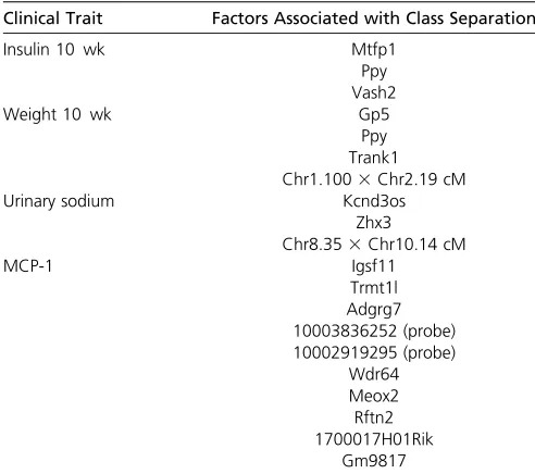
To investigate the factors potentially driving class separa-tion for each of the four phenotypes shown in Figure 5, we evaluated associations for 40,572 expression probes, and two-way interactions between markers as described inlcQTL mapping. The topN¼50 associations were considered in the stepwise regression. Table 4 lists the factors associated with classification found by our procedure for each of the four clinical traits.
Some of the genes associated with the classification of the clinical traits are known to be related to diabetes. Pyy, for example, associated with the classification of insulin and glucose at 10 weeks, is known to be an early indicator of Type II diabetes (Viardotet al.2008). Pitnneret al.(2004) have also shown that Pyy administration reduces body weight gain and glycemic indices in diverse rodent models
of metabolic disease, and thus may be used as a therapeutic target of obesity (De Silva and Bloom 2012). Karra et al.
(2009) showed that low circulating Pyy concentrations pre-dispose mice and humans to the development and/or main-tenance of obesity. Another factor, Gp5, is known to be involved in fasting blood glucose in patients with Type II diabetes (Aleilet al.2008).
Discussion
With advances in technologies for genotyping and phenotyp-ing, QTL mapping studies involving thousands of markers and traits are becoming increasingly common. Such studies pro-vide an unprecedented opportunity to identify more refined genetic models, but, to do so, advances in QTL mapping techniques are required. This work addresses the situation in which a population of interest is not well described by a single genetic model, due to the presence of genetically distinct subpopulations (which we have referred to as classes). As we discuss in the Introduction, standard QTL mapping methods accommodate such situations when the subclasses are well defined by known covariates (e.g., age and sex). On the other hand, when the presence and/or nature of sub-classes are unknown, the lcQTL mapping method developed here is expected to prove useful.
Specifically, the simulation and case studies presented suggest that lcQTL mapping is effective at identifying the correct number of subclasses within a population when two subclasses are present, and does not hinder efficiency if applied to data with one common class. Accurate estimation of the genetic model in the case of one or two classes is also achieved. While lcQTL could, in theory, be applied to identify three or more classes, sample sizes such as those considered here are a limiting factor, and we did not evaluate the per-formance of lcQTL in this setting. In cases where two classes are identified, it will be of interest to determine potential factors affecting the genetic differences between classes; to-ward this end, a number of methods may prove useful. We have detailed one straightforward approach that amounts to testing for association between candidate factors and class membership. Once candidate factors are identified, stepwise regression is used to determine which factors, if any, suffi-ciently explain class differences. While this approach per-formed well in proof-of-principle experiments (where sex was known to separate the class, for example), other ap-proaches that consider groups of traits simultaneously may further improve the sensitivity with which factors may be identified. Automated methods for determining the number of candidates considered should also prove useful, and exten-sions to accommodate multiple trait distributions would broaden the applicability of lcQTL mapping.
As presented, lcQTL mapping assumes that, perhaps fol-lowing appropriate transformation, phenotypes are normally distributed conditionally on genotype. It would be relatively straightforward to accommodate responses that follow other distributions, such as Bernoulli or other distributions from the
Table 4 Factors associated with classes identified by lcQTL for insulin at 10 weeks, weight at 10 weeks, urinary sodium, and MCP-1 in the mouse F2 intercross of Wanget al. (2011) and Tu
et al.(2012)
Clinical Trait Factors Associated with Class Separation
Insulin 10 wk Mtfp1
Ppy Vash2
Weight 10 wk Gp5
Ppy Trank1 Chr1.1003Chr2.19 cM
Urinary sodium Kcnd3os
Zhx3
Chr8.353Chr10.14 cM
MCP-1 Igsf11
Trmt1l Adgrg7 10003836252 (probe) 10002919295 (probe)
Wdr64 Meox2 Rftn2 1700017H01Rik
exponential family (Grun and Leisch 2008). A more important but related consideration is identifiability. While it is well known that mixtures of univariate normal and exponential distributions are identifiable (Leisch 2004), mixtures of dis-crete or continuous uniform distributions are not. Although we assume conditional normality of the data, and we perform transformations if necessary prior to analysis, this assumption should be checked (via qq-plots or normality tests, such as Shapiro-Wilk, Kolmogorov-Smirnov, Lilliefors and Anderson-Darling tests (Razali and Wah 2011)) since extreme viola-tions could result in two-classes being falsely identified.
In summary, lcQTL mapping is expected to prove useful in numerous QTL mapping studies where latent subclasses of subjects defined by distinct genetic models exist. It gives insight into the genetic structures underlying the classes discovered, and improves the percentage of variance explained by the full genetic model. Future work on improving the sensitivity of factors associated with class discovery, and on extending lcQTL to multiple trait distributions, is underway.
Acknowledgments
The authors thank Gary Churchill and Ning Leng for conver-sations that helped motivate creation of the article. This work is supported by National Institutes of Health grant NIH GM102756, and National Science Foundation (NSF) DMS-12-65203, U54 AI117924, DK108259, and DK66369.
Literature Cited
Aleil, B., L. Kessler, N. Meyer, M. L. Wiesel, J. Simeoni et al.,
2008 Plasma levels of soluble platelet glycoprotein V are
linked to fasting blood glucose in patients with type 2 diabetes.
Thromb. Haemost. 100: 713–715.
Broman, K., 2001 Review of statistical methods for qtl mapping in
experimental crosses. Lab Anim. (NY) 30: 44–52.
Broman, K. W., 2003 Mapping quantitative trait loci in the case of
a spike in the phenotype distribution. Genetics 163: 1169–1175.
Dempster, A. P., N. M. Laird, and D. B. Rubin, 1977 Maximum
likelihood from incomplete data via the EM algorithm. J. R. Stat.
Soc. [Ser A] 39: 1–38.
De Silva, A., and S. R. Bloom, 2012 Gut hormones and appetite
control: a focus on PYY and GLP-1 as therapeutic targets in
obesity. Gut Liver 6: 10–20.
Fiara, S., and G. Soromenho, 2010 Fitting mixtures of linear
re-gressions. J. Stat. Comput. Simul. 80: 201–225.
Fraley, C., and A. E. Raftery, 2002 Model-based clustering,
discrim-inant analysis and density estimation. J. Am. Stat. Assoc. 97: 611–
631.
Grun, B., and F. Leisch, 2007 Fittingfinite mixtures of generalized
linear regressions in R. Comput. Stat. Data Anal. 51: 5247–5252.
Grun, B., and F. Leisch, 2009 Finite mixtures of generalized linear
regression models, pp. 205–230 inRecent Advances in Linear
Models and Related Areas, edited by Shalabh, and Christian Heumann. Springer, New York, NY.
Hurvich, C. M., and C. L. Tsai, 1989 Regression and time series
model selection in small samples. Biometrika 76: 297–307.
Karra, E., K. Chandarana, and R. L. Batterham, 2009 The role of
peptide YY in appetite regulation and obesity. J. Physiol. 587: 19–25.
Kass, R. E., and A. E. Raftery, 1995 Bayesian factors. JASA 90:
773–795.
Keller, M. P., Y. Choi, and P. Wang, 2008 A gene expression
net-work model of type 2 diabetes links cell cycle regulation in islets
with diabetes susceptibility. Genome Res. 18: 706–716.
Leisch, F., 2004 Flexmix: a general framework forfinite mixture
models and latent class regression in R. J. Stat. Softw. 11: 1–18.
Mackay, T. F. C., E. A. Stone, and J. F. Ayroles, 2009 The genetics
of quantitative traits: challenges and prospects. Nat. Rev. Genet.
10: 565–577.
Magidson, J., and J. K. Vermunt, 2004 Latent class models, pp.
175–198 inThe Sage Handbook of Quantitative Methodology for
the Social Sciences, edited by D. Kaplan. Sage, Thousand Oaks, CA.
Manichaikul, A., J. Y. Moon, S. Sen, B. S. Yandell, and K. W.
Bro-man, 2009 A model selection approach for the identification of
quantitative trait loci in experimental crosses, allowing epistasis.
Genetics 181: 1077–1086.
Pitnner, R. A., C. X. Moore, S. P. Barvsar, B. R. Gedulin, P. A. Smith et al., 2004 Effects of PYY[3–36] in rodent models of diabetes
and obesity. Int. J. Obes. Relat. Metab. Disord. 28: 963–971.
Razali, N. M., and Y. B. Wah, 2011 Power comparisons of
Sha-piro-Wilk, Kolmogorov-Smirnov, Lilliefors and Anderson-Darling
tests. J. Statist. Model. Anal. 2: 21–33.
Reifsnyder, P. C., G. Churchill, and E. H. Leiter, 2000 Maternal
environment and genotype interact to establish diabesity in
mice. Genome Res. 10: 1568–1578.
Schwarz, G. E., 1978 Estimating the dimension of a model. Ann.
Stat. 6: 461–464.
Sen, S., and G. A. Churchill, 2001 A statistical framework for
quantitative trait mapping. Genetics 159: 371–387.
Tofighi, D., and C. K. Enders, 2008 Identifying the correct number
of classes in growth mixture models inAdvances in Latent
Vari-able Mixture Models, edited by G. R. Hancock, and K. M. Samuel-sen. Information Age Publishing, Inc., Charlotte, NC.
Tu, Z., M. P. Keller, C. Zhang, M. E. Rabaglia, D. M. Greenawalt et al., 2012 Integrative analysis of a cross-loci regulation
net-work identifiesAppas a gene regulating insulin secretion from
pancreatic islets. PLoS Genet. 8: e1003107.
Tueller, S., and G. Lubke, 2010 Evaluation of structural equation
mixture models parameter estimates and correct class
assign-ment. Struct. Equ. Modeling 17: 165–192.
Viardot, A., L. K. Heilbronn, H. Herzog, S. Gregersen, and L. V.
Campbell, 2008 Abnormal postprandial PYY response in
insu-lin sensitive nondiabetic subjects with a strong family history of
type 2 diabetes. Int. J. Obes. 32: 943–948.
Wang, P., J. A. Dawson, M. P. Keller, B. S. Yandell, N. A. Thornberry et al., 2011 A model selection approach for expression
quan-titative trait loci(eQTL) mapping. Genetics 187: 611–621.
Wedel, M., and W. S. DeSarbo, 1995 A mixture likelihood
ap-proach for generalized linear models. J. Classif. 12: 21–55.