Systematic aware learning
A case study in High Energy Physics
VictorEstrade1,∗,CécileGermain1,∗∗,IsabelleGuyon1,3,∗∗∗, andDavidRousseau2,∗∗∗∗
1LRI/TAU, Univ. Paris-Sud/INRIA/CNRS, Université Paris-Saclay, Gif-sur-Yvette, France 2LAL, Univ. Paris-Sud, CNRS/IN2P3, Université Paris-Saclay, Orsay, France
3ChaLearn, Berkeley, USA
Abstract.Experimental science often has to cope with systematic errors that coherently bias data. We analyze this issue on the analysis of data produced by experiments of the Large Hadron Collider at CERN as a case of supervised domain adaptation. Systematics-aware learning should create an efficient repre-sentation that is insensitive to perturbations induced by the systematic effects. We present an experimental comparison of the adversarial knowledge-free approach and a less data-intensive alternative.
1 Introduction
The 21st century extolled the so-called 4th paradigm of science: data-intensive scientific discovery. A subsequent trend is the usage of Machine Learning techniques to actually make use of collected data. On the other hand, since its inception, experimental science has concerned itself with coping with uncertainties. This paper is a followup on [1] where we explore how these two paradigms interact in a specific setting, which issimulation based experimental science, and specifically on the impact of data bias. The principal addition to our previous work is the extended studies of the performances and the use of a more realistic and difficult case study.
In order to be concrete, we focus on a demanding example: the analysis of the data pro-duced by the experiments of the LHC (Large Hadron Collider) at CERN, e.g. the measurement of the characteristics of new particles, such as the Higgs boson. An essential component of this analysis is a procedure for selecting a rare signal over a large background, which is nowadays routinely done with Machine Learning techniques. This selection can be expressed as selecting a region of interest in the space of measured features. Multivariate classification has become the standard tool to optimize the selection region. As such, the classifier is an integral part of the measurement apparatus. For discovery and measurement of a new particle such as the Higgs boson, by definition no labeled real data are available. The classifier has to be trained on simulated data [2].
A typical HEP analysis will report a measurement including two sort of uncertainties: the uncertainty resulting from stochastic effects that we shall call“statistical uncertainty”, and
that resulting from known nuisance factors that we shall call“systematic uncertainty”. A systematics-aware learning procedure should optimize the trade-offbetween both, by learning an efficient representation, which is insensitive, or less sensitive, to perturbations induced by systematic effects. Two strategies are considered in this paper, stemming from the related field of “domain adaptation” [3]: (1) a knowledge-free setting, where the invariant representation is discovered from the data (adversarial supervised learning); or (2) the integration of prior knowledge. The main goal of this paper is to evaluate the two approaches.
In the next section the case study is described especially how the classifier is used inside the analysis workflow. section 3describes the use of domain adaptation methods to tackle systematics. Finallysection 4evaluates and explains the performances of the systematic aware methods.
2 Systematics in simulation-based analysis
We briefly describe the problem setting we are interested in as a machine learning problem, without dwelling into the specifics of the underlying physics.
Classification.We address a two-class problem as in [2]:signal(S) vs.background(B) , theS class, e.g. a specific Higgs boson final state being the “positive” class. To cope with class imbalance (elements of classS are very rare), the simulator produces an even number of examples of the two classes with importance-weights. This allows us to train the classifier on a balanced dataset while taking weights into account for performance evaluation. The quantities of interest are the expected weighted true positive (signal classified as signal) and false positive (background classified as signal) counts where thewiare the weights andtis the classification threshold of the discriminant valuescorei:
s=
S,scorei>t
wi and b=
B,scorei>t
wi.
The weights include luminosity, cross-section, efficiencies and other factors so thatsandbare normalized to what is expected in the collected data, for example in one year of data-taking. In the simplest machine learning settings, data are drawni.i.d.from an unknown, but fixed data distribution. The generalization error in that case combines the modeling error (due to model bias/model finite capacity and finite sample size) and the intrinsic error (lowest achievable by the Bayes optimal classifier). This is termedstatistical error. The type ofsystematic error studied in this paper comes from departures of the data from the classicali.i.d.assumption in the following way: test data may be differently distributed from training data due to known nuisance factors (notedZ), the effect of which is bounded by known values. Typical examples for Z are the cross-section of specific backgrounds predicted by theorists or measured in other experiments or analyses, the efficiency for the detector to identify specific particles, or the calibration of the detector. This coincides with the well known “domain adaptation” problem in machine learning, under the covariate shift paradigm [4], as it coherently biases data.
Figure of merit.We provide in this section the figure of merit used by particle physicists, which is not the classification accuracy, but a non-linear function of the number of true and false positives. We call “signal region” the region of input space classified asS by the classifier. Particle detection in physics boils down to counting the number of events (data samples) falling into the signal region and compare it to expectation. It can be expressed as a measurement of µthe ratio of the number of signal event measured over the expected one. The uncertainty of µshould be minimized. Letszandbzbe the weighted counts of true and false positives with systematics atZ=z. The figure of merit is the relative error:
σµ µ =
that resulting from known nuisance factors that we shall call“systematic uncertainty”. A systematics-aware learning procedure should optimize the trade-offbetween both, by learning an efficient representation, which is insensitive, or less sensitive, to perturbations induced by systematic effects. Two strategies are considered in this paper, stemming from the related field of “domain adaptation” [3]: (1) a knowledge-free setting, where the invariant representation is discovered from the data (adversarial supervised learning); or (2) the integration of prior knowledge. The main goal of this paper is to evaluate the two approaches.
In the next section the case study is described especially how the classifier is used inside the analysis workflow. section 3describes the use of domain adaptation methods to tackle systematics. Finallysection 4evaluates and explains the performances of the systematic aware methods.
2 Systematics in simulation-based analysis
We briefly describe the problem setting we are interested in as a machine learning problem, without dwelling into the specifics of the underlying physics.
Classification.We address a two-class problem as in [2]:signal(S) vs.background(B) , theS class, e.g. a specific Higgs boson final state being the “positive” class. To cope with class imbalance (elements of classS are very rare), the simulator produces an even number of examples of the two classes with importance-weights. This allows us to train the classifier on a balanced dataset while taking weights into account for performance evaluation. The quantities of interest are the expected weighted true positive (signal classified as signal) and false positive (background classified as signal) counts where thewiare the weights andtis the classification threshold of the discriminant valuescorei:
s=
S,scorei>t
wi and b=
B,scorei>t
wi.
The weights include luminosity, cross-section, efficiencies and other factors so thatsandbare normalized to what is expected in the collected data, for example in one year of data-taking. In the simplest machine learning settings, data are drawni.i.d.from an unknown, but fixed data distribution. The generalization error in that case combines the modeling error (due to model bias/model finite capacity and finite sample size) and the intrinsic error (lowest achievable by the Bayes optimal classifier). This is termedstatistical error. The type ofsystematic error studied in this paper comes from departures of the data from the classicali.i.d.assumption in the following way: test data may be differently distributed from training data due to known nuisance factors (notedZ), the effect of which is bounded by known values. Typical examples for Z are the cross-section of specific backgrounds predicted by theorists or measured in other experiments or analyses, the efficiency for the detector to identify specific particles, or the calibration of the detector. This coincides with the well known “domain adaptation” problem in machine learning, under the covariate shift paradigm [4], as it coherently biases data.
Figure of merit.We provide in this section the figure of merit used by particle physicists, which is not the classification accuracy, but a non-linear function of the number of true and false positives. We call “signal region” the region of input space classified asS by the classifier. Particle detection in physics boils down to counting the number of events (data samples) falling into the signal region and compare it to expectation. It can be expressed as a measurement of µthe ratio of the number of signal event measured over the expected one. The uncertainty of µshould be minimized. Letszandbzbe the weighted counts of true and false positives with systematics atZ =z. The figure of merit is the relative error:
σµ µ =
σ2sta+σ2sys, (1)
whereσsta=s−01√s0+b0is the relative statistical error andσsys =s−01(sz+bz−s0−b0) the relative systematic error. The nuisance parameterZis 0 in the nominal case (this is just a notation); they assumption is thatszandbzare approximately linear withZover the interval of interest.
This expression can be formally derived with the profile likelihood ratio method [5]. An intuitive explanation works as follows. LetNbe the selected events,i.e. N = s+b. N is assumed to follow a Poisson distribution. The measurementµis proportional to number of signal events, and normalized to the expected one from the standard model, that isµ0 =1. The systematic error is by definitionµz−µ0. Because the value of the Nuisance Parameter is unknown, the best estimate of the number of signal events atZ =zisNz−b0, obtained by subtracting the nominal number of background events, yielding:
σsys= sz+bz−s s0−b0 0
The statistical error measures the impact of the intrinsic deficiencies of the selection procedure. In the real experiment, all we have isN, thus the relative statistical error is the ratio of the Poisson variance to the nominal estimate of the number of signals:
σsta=
√
s0+b0 s0 .
The dataset.In the experiments, we use the HiggsML challenge dataset [2], available in [6] which corresponds to nominal data. Similar experiments are possible using the Enhanced Higgs Boson toτ+τ−Dataset [7] [8]. The software [9] to compute the impact of the Nuisance parameter on the simulation is described in [10]. In the following this will be calledskewing the data. In a few words : the energy measurement of one particle, theτhadronic decay, is skewed by a fixed factor up to 10%, the missing transverse energy is skewed accordingly, as well as the high level quantities (i.e. invariant masses).
3 Domain adaptation to reduce systematics
The setting presented insection 2corresponds to domain adaptation [3] where the perturbation induced by the systematic effect drives the experimental data distribution (target) away from the simulation data (source). Recent works [11], [12] often apply semi-supervised domain adaptation to take advantage of available labeled data to train a model to perform well on similar data with few or no labels.
The systematic aware setting can profit from a fully supervised adaptation since, at training time, we have all the labels and the nuisance parameter values. But we do not know among all the possible distributions (targets) which one will be produced during the experiment. In practice testing all possible values for every nuisance parameters is intractable due to combinatorial explosion.
We shortly describe and compare three methods : a "naive" data augmentation, adversarial training and the integration of a priori knowledge as a regularization.
Data Augmentation.Since we face a fully supervised setting a simple solution is to train the model on a mix of all possible target distributions. Given enough capacity and training data the model should learn a boundary resilient to the systematic effect. But the resulting mixture is very noisy which could in practice result in a loss of performance.
parameter. This is enforced by a bi-objective loss penalizing the classification error and the ability of an adversarial network to reconstructZfrom the output of the classifier. The trade-off between both losses is controlled by an hyper-parameterλ. It enjoys the same theoretical optimality results in an equal opportunity [16] model. To train the adversary, and extract meaningful gradient from it, Pivot method also requires mixture of data that span the possible values of the nuisance parameter
Knowledge integration.Tangent Propagation [17] proposes to integrate a priori knowl-edge of some geometric invariant in the loss. A regularization is computed from the partial derivative of the classifier output with respect to the geometric transformation parameter. Same as Pivot the trade-offbetween the regularization and the classification error is controlled by an hyper-parameterλ. If the systematics is not a differentiable transformation it is possible to compute tangents with finite differences. This approach requires only nominal data and the tangents making it less data-greedy than the previous ones.
4 Experimental results
In this section the performances of systematic-aware methods (data augmentation, tangent propagation and pivot adversarial) will be compared to the baselines (standard neural network and gradient boosting).
4.1 Setting
All neural network’s architectures are similar to ensure fair comparison of the performances. This architecture is composed of 3 hidden layers with 120 ReLU activated neurons except for Tangent Propagation that is using Softplus activations for it is twice differentiable. All methods uses Adam optimizer with default parameters and a batchsize of 1024. GB parameters are 1000 trees of maximum depth 3 and learning rate 0.1. This configuration has been selected with grid search to minimize the statistical error of the baselines.
The baselines are trained on the nominal data only while Pivot and Data Augmentation are trained on skewed data with, for each event,Zdrawn from a normal distribution centered on zero (the nominal value) with its spread left as an hyper-parameter and Tangent Propagation is trained on the nominal data with the tangent vectors computed using finite differences.
The test set is skewed with aZtest = +3% unknown beforehand. Other values ofZtest have been tried and gave similar results with the expected effect that the furtherZis from the nominal value the larger the systematic error.
The score extracted from the classifier requires the choice of a threshold to compute the figure of merit. The figure of merit is therefore computed for every possible threshold and plotted according to the number of events remaining in the selected region. The threshold optimization is left for future work.
Presented results are means along a seeded 12 random split cross validation (20% testing, 80% training). The split is done before any preprocessing since the cut can remove samples from the dataset. Some curves are slightly smoothed to help visualization.
4.2 Overall performances
parameter. This is enforced by a bi-objective loss penalizing the classification error and the ability of an adversarial network to reconstructZfrom the output of the classifier. The trade-off between both losses is controlled by an hyper-parameterλ. It enjoys the same theoretical optimality results in an equal opportunity [16] model. To train the adversary, and extract meaningful gradient from it, Pivot method also requires mixture of data that span the possible values of the nuisance parameter
Knowledge integration.Tangent Propagation [17] proposes to integrate a priori knowl-edge of some geometric invariant in the loss. A regularization is computed from the partial derivative of the classifier output with respect to the geometric transformation parameter. Same as Pivot the trade-offbetween the regularization and the classification error is controlled by an hyper-parameterλ. If the systematics is not a differentiable transformation it is possible to compute tangents with finite differences. This approach requires only nominal data and the tangents making it less data-greedy than the previous ones.
4 Experimental results
In this section the performances of systematic-aware methods (data augmentation, tangent propagation and pivot adversarial) will be compared to the baselines (standard neural network and gradient boosting).
4.1 Setting
All neural network’s architectures are similar to ensure fair comparison of the performances. This architecture is composed of 3 hidden layers with 120 ReLU activated neurons except for Tangent Propagation that is using Softplus activations for it is twice differentiable. All methods uses Adam optimizer with default parameters and a batchsize of 1024. GB parameters are 1000 trees of maximum depth 3 and learning rate 0.1. This configuration has been selected with grid search to minimize the statistical error of the baselines.
The baselines are trained on the nominal data only while Pivot and Data Augmentation are trained on skewed data with, for each event,Zdrawn from a normal distribution centered on zero (the nominal value) with its spread left as an hyper-parameter and Tangent Propagation is trained on the nominal data with the tangent vectors computed using finite differences.
The test set is skewed with aZtest = +3% unknown beforehand. Other values ofZtest
have been tried and gave similar results with the expected effect that the furtherZis from the nominal value the larger the systematic error.
The score extracted from the classifier requires the choice of a threshold to compute the figure of merit. The figure of merit is therefore computed for every possible threshold and plotted according to the number of events remaining in the selected region. The threshold optimization is left for future work.
Presented results are means along a seeded 12 random split cross validation (20% testing, 80% training). The split is done before any preprocessing since the cut can remove samples from the dataset. Some curves are slightly smoothed to help visualization.
4.2 Overall performances
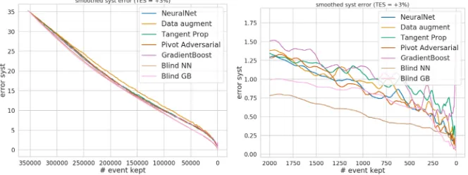
The standard neural network surprisingly reduces best the figure of merit near the minimum. Figure 1 shows that Tangent propagation is the worse method although its regularization should make the classifier less sensitive to the systematic effect. Pivot and data augmentation give similar performances as the standard neural network. The remains of this section is to explore possible reasons behind the poor performances systematic aware methods.
Figure 1: Figure of merit (σµµ) reported according to the number of selected events. Right : a zoom near the minimum.
4.3 Effect of the cut
None of the systematic aware methods gave better results than a regular neural network. We introduce two new methods, for illustrative purpose only, that will artificially remove the domain shift on variables. On the HiggsML dataset only 8 variables are prone to the systematic effect leaving 21 variables unchanged. Ablindneural network and ablindgradient boosting model are trained using these 21 insensitive variables; these models using less variables will be less sensitive on the statistical point of view.
InFigure 2the systematic error is not zero forblind models which shows that there is another source of systematic error.
Figure 2: Systematic error (sz+bz−s0−b0
s0 ) comparison between Blind models and regular models.
Although the blind models are insensitive to the variable skewing the systematic error is not zero.
theblindmodels show zero systematic error leading to the conclusion that the systematic error is a combination of 2 sources : the domain shift on the variables and the cut.
Without the cut the performances (Figure 3) are better but near the minimum most of the events are rejected including events that could appear or disappear because of the cut making systematic effect caused by the cut negligible. This rejects the hypothesis that the cut is responsible for the lack of improvement of the systematic aware methods.
Figure 3: Figure of merit (σµ
µ) without the 22 GeV cut. Only statistical error remains for the
Blind models. Other methods have to cope with domain shift on variables and statistical error.
4.4 Systematic aware learning
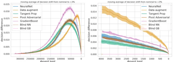
Near the optimum the systematic aware methods do not beat the baseline even when the cut is removed from the problem. The robustness of the score function against the skewing of the variables can be measured by computing the difference of the score given by a model between en eventxiand the same event after skewingskew(xi).
Figure 4reports a moving average of the absolute decision difference between skewed and nominal data according to the selection threshold and shows that each models is more or less robust according to the chosen threshold. Tangent propagation and data augmentation are improving robustness to the systematic effect but not on the final selected region. Moreover Pivot adversarial network is clearly imitating the neural network.
theblindmodels show zero systematic error leading to the conclusion that the systematic error is a combination of 2 sources : the domain shift on the variables and the cut.
Without the cut the performances (Figure 3) are better but near the minimum most of the events are rejected including events that could appear or disappear because of the cut making systematic effect caused by the cut negligible. This rejects the hypothesis that the cut is responsible for the lack of improvement of the systematic aware methods.
Figure 3: Figure of merit (σµ
µ) without the 22 GeV cut. Only statistical error remains for the
Blind models. Other methods have to cope with domain shift on variables and statistical error.
4.4 Systematic aware learning
Near the optimum the systematic aware methods do not beat the baseline even when the cut is removed from the problem. The robustness of the score function against the skewing of the variables can be measured by computing the difference of the score given by a model between en eventxiand the same event after skewingskew(xi).
Figure 4reports a moving average of the absolute decision difference between skewed and nominal data according to the selection threshold and shows that each models is more or less robust according to the chosen threshold. Tangent propagation and data augmentation are improving robustness to the systematic effect but not on the final selected region. Moreover Pivot adversarial network is clearly imitating the neural network.
Figure 4: Moving average of the score difference between nominal data and skewed data (Z=3%).
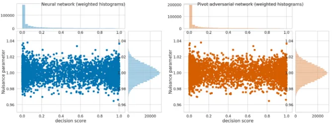
This last statement is also suggested by the lack of visible relation between the classification score and the nuisance parameter (illustratedFigure 5). This indicate that the adversarial task is very difficult which is why this method fails to improve on the baseline. Indeed, even training a neural network or gradient boosting to separate nominal data from skewed data gave very poor results (55% accuracy at most withZ =±10%). To the best of our knowledge, the Pivot method is successful (in the original paper [13] or in [15] ) only when the nuisance parameter is one of the input or can be regressed from the inputs.
Figure 5: Score vs nuisance parameter for trained neural network (left) and Pivot adversarial method (right). Each dot is single event for which we report its classification score and the value of the nuisance parameter used to produce it.
Improving the robustness of the classifier score function against the domain shift does not have the expected impact on the figure of merit. Improving the robustness of the classifier score function against the domain shift does not have the expected impact on the figure of merit. Reaching the minimum ofσµrequires to reject most of the data to get a very pure
sample of signals, whereas the systematic aware methods are trained to become robust on the entire dataset. Moreover the link between the classification score function and the accuracy of the measurement is complex. These results may suggest that a robust score function is not necessary for an accurate measurement.
5 Conclusion
This paper has presented a case study of data bias in simulation-based experimental science, and related it to the classical concepts of domain adaptation, systematic error and nuisance pa-rameters. The problem consists of learning a representation that is insensitive to perturbations induced by nuisance parameters. Include invariant properties as a regularization (TP) training on a mixture of simulations turned out to waste efforts on data that is rejected by the analysis pipeline therefore not included in the figure of merit. Learning regularization with adversarial training is as difficult as finding a learnable objective for the adversary.
These conclusions leads the possible improvement like regularize only on a subsection of the data that is likely to be in the final selection region. Direct optimization of the figure of merit will also be explored in future studies.
References
[1] V. Estrade, C. Germain, I. Guyon, D. Rousseau,Systematics aware learning: a case
study in High Energy Physics, inESANN 2018 - 26th European Symposium on Artificial
[2] C. Adam-Bourdarios, G. Cowan, C. Germain, I. Guyon, B. Kégl, D. Rousseau,The Higgs boson machine learning challenge, inNIPS 2014 Workshop on High-energy Physics and Machine Learning(Montreal, Canada, 2014), Vol. 42 ofJMLR: Workshop and Conference Proceedings, pp. 19–55
[3] S. Ben-David, J. Blitzer, K. Crammer, A. Kulesza, F. Pereira, J.W. Vaughan, Machine Learning79, 151 (2010)
[4] H. Shimodaira, Journal of Statistical Planning and Inference90, 227 (2000)
[5] G. Cowan, K. Cranmer, E. Gross, O. Vitells, The European Physical Journal C71, 1554 (2011)
[6] A. collaboration,Dataset from the atlas higgs boson machine learning challenge 2014,
http://opendata.cern.ch/record/328(2014) [7] P. Baldi, P. Sadowski, D. Whiteson (2014),1410.3469
[8] P. Baldi, P. Sadowski, D. Whiteson, Dataset from the enhanced higgs boson to τ+τ−search with deep learning,http://mlphysics.ics.uci.edu/data/htautau/ (2015)
[9] V. Estrade, D. Rousseau,Datawarehouse for systematic effect on toys and open access datasets,https://doi.org/10.5281/zenodo.1887847
[10] V. Estrade, C. Germain, I. Guyon, D. Rousseau, Adversarial learning to eliminate systematic errors: a case study in High Energy Physics, in NIPS 2017 - workshop Deep Learning for Physical Sciences (Long Beach, United States, 2017), pp. 1–5,
https://hal.inria.fr/hal-01665925
[11] Y. Ganin, E. Ustinova, H. Ajakan, P. Germain, H. Larochelle, F. Laviolette, M. Marchand, V. Lempitsky, arXiv:1505.07818 [cs, stat] (2015), arXiv: 1505.07818
[12] N. Courty, R. Flamary, D. Tuia,Domain adaptation with regularized optimal transport, inECML/PKDD 2014(2014), LNCS, pp. 1–16
[13] G. Louppe, M. Kagan, K. Cranmer, arXiv:1611.01046 [physics, stat] (2016), arXiv: 1611.01046
[14] I.J. Goodfellow, J. Pouget-Abadie, M. Mirza, B. Xu, D. Warde-Farley, S. Ozair, A. Courville, Y. Bengio, arXiv:1406.2661 [cs, stat] (2014), arXiv: 1406.2661
[15] [The Atlas Collaboration],Performance of mass-decorrelated jet substructure observ-ables for hadronic two-body decay tagging in atlas, ATL-PHYS-PUB-2018-014 (2018) [16] M. Hardt, E. Price, N. Srebro,Equality of Opportunity in Supervised Learning, inNIPS
(2016)
[17] P.Y. Simard, B. Victorri, Y. LeCun, J.S. Denker,Tangent Prop - A Formalism for Specify-ing Selected Invariances in an Adaptive Network., inNIPS, edited by J.E. Moody, S.J. Hanson, R. Lippmann (Morgan Kaufmann, 1991), pp. 895–903, ISBN 1-55860-222-4,