Synthesis of Linear Antenna Arrays using Accelerated
Particle Swarm Optimization algorithm
P.V.Florence
Department of ECE AU College of Engineering (A)
Andhra University Visakhapatnam, India
G S N Raju
, PhDDepartment of ECE AU College of Engineering (A)
Andhra University Visakhapatnam, India
ABSTRACT
In the present work, pattern synthesis of linear arrays using APSO is presented. APSO algorithm is employed for the synthesis of uniformly spaced arrays of two classes using unequal phases with equal amplitudes and with unequal amplitudes. The main objective of this work is to minimize the sidelobe level with a constraint on beam width and to perform null steering for isotopic linear antenna arrays by controlling different parameters of the array elements. The results are compared with the patterns of uniform linear array. The sidelobe level is reduced for amplitude-phase synthesis when compared with phase only synthesis as the number of elements are increased in an array. The patterns are numerically computed for different number of elements.
Keywords
Pattern synthesis, Sidelobe level, Beam width, Accelerated Particle Swarm Optimization.
1.
INTRODUCTION
Synthesis of linear antenna arrays with a desired radiation pattern has been extensively studied over the last few decades [1-4]. Radiation pattern depends on the number and type of elements being used, the physical and electrical structure of the array etc., [5]. Large arrays have been employed to gain high directivity in order to design a high performance antenna. Patterns with minimal beam width, optimum SLL and null control can fulfill the high gain demand and ensures the reduction of the inter channel interferences. Maximum SLL reduction is achieved by changing either or both the amplitudes and phases of the elements which are desirable in many applications such as satellite, radar and communication systems.
Several pattern synthesis methodologies are obtained using phase only control have been described [6-10]. Phase only beam shaping in a uniformly spaced array has been presented by Chakrabarty [11]. In [12], numerical search technique is used to minimize the pattern sidelobe level by phase only synthesis for linear and planar arrays. F. Ares [13] employed a new way of applying the Woodward Lawson technique to generate multiple radiation patterns with different phase excitations and prefixed amplitude distributions. K.Lee [14] reported a novel stochastic approach called as Electromagnetism like algorithm for phase only synthesis of antenna arrays. In [15], the synthesis method of linear array geometry with minimum SLL and null control using Particle Swarm Optmization (PSO) was described. Linear array synthesis using Taguchi method and Self adaptive DE has been presented by Dib [16].
Marcano [17] reported the technique of synthesizing complex radiation pattern of a linear and planar arrays using Genetic Algorithm (GA). A comparative study is made between phase only and amplitude-phase synthesis using floating point GA in [18]. Mandal [19] described a design of linear antenna array with shaped power pattern using Modified Differential Evolution (DE) algorithm.
Sidelobe nulling in linear array patterns with phase only control are presented [20-21]. In [22], Genetic algorithm is employed for placing of nulls in the direction of interference with phase only synthesis. A modified GA is proposed for the design of phase only linear array with simultaneous null steering and maximum sidelobe level minimization [23]. Design procedure for pattern synthesis of the linear antenna arrays with multilobe pattern and adaptive nulling using sequential quadratic programming algorithm is reported [24]. Goudos investigated on the synthesis of unequally spaced linear array with SLL suppression under constraints to beam width and null control using Comprehensive Learning Particle Swarm Optimizer [25]. Guney used the Seeker Optimization technique for the pattern synthesis of linear antenna arrays with prescribed nulls [26].
In the present work, Accelerated Particle Swarm Optimization (APSO) [27], a variant of Particle Swarm Optimization (PSO) is employed for linear array synthesis by finding the optimum amplitude and phase values of the array elements with equal spacing. The desired goal is to minimize the pattern characteristics such as SLL with the constraint of beam width, equal to that of a uniform linear array and to produce nulls in the desired directions. The result obtained has shown the applicability of the APSO to antenna design problems. It is obtained that the amplitude-phase synthesis is superior to phase only synthesis. Desired unidirectional and bi-directional nulls are produced at specific directions with phase only control.
The rest of this paper is organized as follows. In Section II, the synthesis of linear antenna array geometry, Formulation of the array factor and Fitness function are explained. Section III, deals with the concepts of Accelerated Particle Swarm Optimization. The synthesized patterns with minimal sidelobe level and null steering for different array elements are presented in Section IV. Finally, the conclusions are drawn in Section V.
2.
PROBLEM FORMULATION
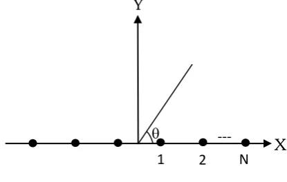
constraint on beam width and to perform null steering with reduced SLL. A 2N element linear array placed along X-axis with uniform spacing is considered as shown in Fig1.
Fig 1: Geometry of 2N element symmetric linear array
For symmetric array, the array factor
AF
is given by
cos 5 . 0 n cos j exp w 2 AF N 1 n n n (1)Here, wn represents the excitation amplitude of the nth element of the array,n represents the excitation phase of the nth element of the array, N is the number of elements in the array and
denotes the azimuth angle.The normalized array factor in dB can be expressed as
AF
max
AF
log
20
)
(
AF
n 10(2)
The array is synthesized using APSO. The fitness function used for maximal SLL minimization under the constraint on beam width is defined as follows
(3) FNBW FNBW to subject 2 , 0 AF M inimize = Fitness 1 I d n Here, FNBWd is the first null beam width of the pattern
produced by the array considered for optimization. FNBWI=1
represents the corresponding values obtained with the uniformly excited array of similar size.
The fitness function to SLL reduction under the constraint of null steering is defined as follows
k1 fSL k2 fNS Fitness (4) Here 1
k
and 2k
are the weights, first term is for suppressing the maximal SLL of the array pattern defined as
n
SL maxAF
f (5) Here,
SL
f is the fitness function which denotes the feasible
region excluding the main lobe. The second term in the equ. (4) is for null steering defined as
k k null n NS AFf (6)
Here,
NS
f is the fitness function for nulls in the direction of
the kth null.
3.
ACCELERATED PARTICLE SWARM
ALGORITHM
PSO refers to a relatively new family of algorithms that may be used to find the optional solutions to numerical problems. It was introduced by Russel Eberhart and James Kennedy in the year 1995. PSO is an evolutionary algorithm inspired by imitating social behavior of schools of fish or flocks of birds [28]. PSO consists of agents called particles where each particle represents a potential solution in the search space. Interaction and sharing of information among the particles is the main source of swarms searching capability. All the particles are allowed to move systematically in the search space. The basic principle in their algorithm is that each and every particle adjusts its coordinates according to its own experience and that of the other particles. This implies that each particle has memory of its own or self best position called as pbest. Another best value obtained so far by the neighbourhood experiences is called as gbest.
The working of PSO is associated with velocity vector component and position vector component. The position and velocity of the particles are updated by using the following equations.
gbest X t
r c t X pbest r . c t V . w 1 t V n 2 2 n n 1 1 n n (7)
t 1 X
t V
t 1Xn n n (8) Here, w is the inertia coefficient of the particle which plays an important role in PSO was introduced by Eberhart and Shi [29].Vn
t1 is the current particle’s velocity, Vn
t is theprevious particle’s velocity, Xn
t1 is the current particle’s position, Xn
t is the previous particle’s position.r
1and r are 2uniformly distributed random numbers in the range [0,1]. c1
and c2 are the acceleration constants which control the relative effect of the pbest and gbest particles. pbestnis the
current pbest value, gbest is the current gbest value. The PSO algorithm is developed in 4 steps which will stop when the exit criteria is met. The pseudo code of the PSO is shown below:
Step1: Initialize the swarm population within the search space with random positions and velocities.
Step 2: Evaluate the fitness of each particle in the swarm. Step 3: Repeat for each particle in the swarm.
Step 3.1: Find the pbest value and calculate the fitness value. If pbest in current interaction > previous pbest value then pbest is the current pbest value obtained.
End if
Step 3.2: Find the gbest value from the best fitness value obtained among all the pbest values.
Step 3.3: Update velocity of the particle using equ. (7). Step 3.4: Update position of the particle using equ. (8). Step 4: Repeat step 3.1 through 3.4 until the end criteria is met.
Y
N
2
1
In recent years, various attempts have been made to improve the performance of standard PSO. One among the variants of PSO is APSO which extends the standard PSO algorithm. The standard PSO uses both pbest and gbest value. In APSO, only gbest is used as it could accelerate the convergence of the algorithm. The version of APSO was introduced by Xin She Yang in the year 2008. The position and velocity vectors of the particles are initialized randomly and are updated with time. The velocity vector is generated by using the following equation.
t 1 w.V
t .c .
gbest X
t
Vn n n n (9) Here
c
n is the random variable chosen between the interval (0,1).The position vector is updated by using the following equation
t 1 X
t V
t 1Xn n n (10)
In order to increase the convergence even further, the above two equations are combined into a single equation which is given by
n nn t 1 1 X t .gbest .c
X (11) The typical values of APSO are = 0.1 to 0.4 and = 0.1 to 0.7. Here is taken as 0.2 and as 0.5. The advantage of using this algorithm is to reduce the randomness as the numbers of iterations proceed. This can be done by using a monotonically decreasing function given by
0
1
t
(12)Here
is the control parameter which is taken as 0.97 and t is the number of iterations or time steps where
max
t , 0
t and
max
t
is the maximum value of the iterations. The pseudo code for APSO is as shown below:Step1: Initialize the swarm population within the search space with random positions and velocities.
Step 2: Evaluate the fitness function of each particle in the swarm.
Step 3: Repeat for each particle in the swarm. Step 3.1: Find the gbest value.
Step 3.2: Evaluate the position of the particle using the equ. (11).
Step 4: Repeat step 3.1 through 3.2 until the end criteria is met.
4.
RESULTS
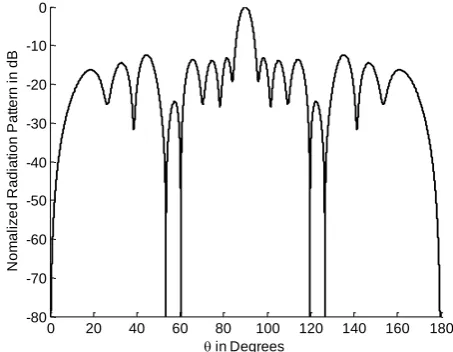
The simulated results for various linear array designs are obtained using APSO algorithm. APSO is initialized by taking random values of excitation coefficients for amplitude control to be in the range (0, 1) and phase control to be in the range of (-π, π) with uniform spacing of 0.5 between the elements. The optimized amplitudes and phases are given in Table1-2. The corresponding normalized radiation patterns for an element array of 20 and 40 are depicted in the Figs. (2-5). From the Fig.(2) it is evident that the maximum SLL for phase only synthesis for 20 element array is lower by about 2.24dB (from -13.18dB to -15.42dB) and for amplitude-phase synthesis is lower by about 2.46dB (from -13.18dB to -15.64 dB). Similarly, for 40 element array the SLL is lower by about
2.64dB for phase only synthesis and 3.13dB for amplitude-phase synthesis. All the results are compared with uniformly excited linear array (ULA). The comparative results for phase only and amplitude-phase are shown in Table3. The results reveal that synthesized patterns for amplitude-phase synthesis offer a considerable SLL reduction without deteriorating the beam width when compared with phase only synthesis. The second goal of phase only synthesis discuss the optimum sidelobe reduction under constraint of null steering at a specific direction. The desired null is less than -60dB and the desired null direction is at 140º. Figs.(6-7) show the final optimum array patterns of 20 and 40 elements respectively. The dashed line in Fig.(6) depicts the pattern of the 20 element array by phase only synthesis without constraint of null steering and the final maximal SLL is about -15.96dB at 140º. The solid line represents the optimum maximal SLL of 20 element array becomes -13.01dB with a constraint of null steering. After imposing the null on the 20 element array, the final optimum maximum SLL is reduced by 2.95dB. The final optimum SLL is reduced by about 2.22dB for 40 element array.
Bidirectional null steering is applied on a 20 element array. The sidelobe reduction under the constraint of null steering at two specific directions by phase only synthesis is considered. The optimum phase values are presented in Table 4. Fig.(8) depicts the final optimum pattern of 20 element array with the constraint of bidirectional null steering. The solid line in Fig.(8) represents the result of two directions of null steering chosen as 120º and 125º.
Table 1: Element phases and amplitudes of 20 element array derived using the APSO algorithm.
N
Phase only
Synthesis Amplitude-Phase Synthesis
Phases(deg) Amplitudes Phases(deg)
1 8.5600 0.6570 -52.6777
2 2.8361 0.6245 -49.8359
3 21.3771 0.9255 -42.2155
4 -2.9393 0.6300 -61.2549
5 24.8320 0.5960 -61.7305
6 -45.2923 0.3486 -93.5239
7 4.0451 0.9323 -41.0295
8 55.3076 0.6105 3.0424
9 2.1715 0.8228 -78.8906
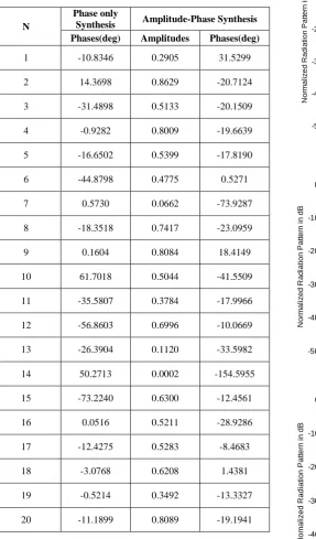
Table 2: Element phases and amplitudes of 40 element array derived using the APSO algorithm.
N
Phase only
Synthesis Amplitude-Phase Synthesis
Phases(deg) Amplitudes Phases(deg)
1 -10.8346 0.2905 31.5299
2 14.3698 0.8629 -20.7124
3 -31.4898 0.5133 -20.1509
4 -0.9282 0.8009 -19.6639
5 -16.6502 0.5399 -17.8190
6 -44.8798 0.4775 0.5271
7 0.5730 0.0662 -73.9287
8 -18.3518 0.7417 -23.0959
9 0.1604 0.8084 18.4149
10 61.7018 0.5044 -41.5509
11 -35.5807 0.3784 -17.9966
12 -56.8603 0.6996 -10.0669
13 -26.3904 0.1120 -33.5982
14 50.2713 0.0002 -154.5955
15 -73.2240 0.6300 -12.4561
16 0.0516 0.5211 -28.9286
17 -12.4275 0.5283 -8.4683
18 -3.0768 0.6208 1.4381
19 -0.5214 0.3492 -13.3327
[image:4.595.322.533.75.242.2]20 -11.1899 0.8089 -19.1941
Fig. 2 Normalized radiation patterns for N=20.
[image:4.595.260.532.80.642.2]
Fig. 3 Normalized radiation patterns for N=40.
Fig. 4 Normalized radiation patterns for N=20.
0 20 40 60 80 100 120 140 160 180 -50
-40 -30 -20 -10 0
in Degrees
N
o
rm
a
li
ze
d
R
a
d
ia
ti
o
n
P
a
tt
e
rn
i
n
d
B
ULA Phase only
0 20 40 60 80 100 120 140 160 180 -50
-40 -30 -20 -10 0
in Degrees
N
o
rm
a
li
ze
d
R
a
d
ia
ti
o
n
P
a
tt
e
rn
i
n
d
B
ULA Phase only
0 20 40 60 80 100 120 140 160 180 -50
-40 -30 -20 -10 0
in Degrees
N
o
m
a
li
ze
d
R
a
d
ia
ti
o
n
P
a
tt
e
rn
i
n
d
B
ULA
[image:4.595.48.336.109.599.2]Fig. 5 Normalized radiation patterns for N=40.
Fig. 6 Optimum pattern of 20 element array by phase only synthesis with unidirectional null steering and without
[image:5.595.56.282.281.460.2]null steering
Fig. 7 Optimum pattern of 40 element array by phase only synthesis with unidirectional null steering and without
null steering
Fig. 8 Optimum pattern of 20 element array by phase only synthesis with the constraint of bidirectional null steering
Table3: Comparative results for phase only and amplitude-phase synthesis
N
Phase only Synthesis
Amplitude-Phase Synthesis SLL
(dB)
FNBW (deg)
SLL (dB)
FNBW (deg)
20 -15.42 11.51 -15.64 11.51 40 -15.88 5.80 -16.37 5.80
Table 4: Element phases of 20 element uniform amplitude array with bidirectional null steering at 120 and 125
degrees
N Phases (deg)
1 -40.2847
2 -55.9952
3 -34.6468
4 -54.5513
5 -114.1676
6 -61.0429
7 -44.7537
8 -65.2943
9 -29.9485
10 -116.3448
0 20 40 60 80 100 120 140 160 180 -50
-40 -30 -20 -10 0
in Degrees
N
o
m
a
li
ze
d
R
a
d
ia
ti
o
n
P
a
tt
e
rn
i
n
d
B
ULA
Phase-Amplitude
0 20 40 60 80 100 120 140 160 180 -80
-70 -60 -50 -40 -30 -20 -10 0
in Degrees
N
o
m
a
li
ze
d
R
a
d
ia
ti
o
n
P
a
tt
e
rn
i
n
d
B
without null steering with null steering
0 20 40 60 80 100 120 140 160 180 -80
-70 -60 -50 -40 -30 -20 -10 0
in Degrees
N
o
m
a
li
ze
d
R
a
d
ia
ti
o
n
P
a
tt
e
rn
i
n
d
B
without null steering with null steering
0 20 40 60 80 100 120 140 160 180 -80
-70 -60 -50 -40 -30 -20 -10 0
in Degrees
N
o
m
a
li
ze
d
R
a
d
ia
ti
o
n
P
a
tt
e
rn
i
n
d
[image:5.595.358.494.473.714.2] [image:5.595.55.280.516.691.2]5.
CONCLUSIONS
It is evident from the results that APSO is successfully used to design arrays. Two cases of linear array design have been considered; phase only optimization and amplitude-phase optimization. Simulation results show that the amplitude-phase synthesis resulted in reduced sidelobe levels compared to that of the phase-only synthesis with a constraint of beam width. Sidelobe level reduction under the constraint of null steering at a specific direction is obtained with phase only synthesis. It is observed from the results that the constraints of null steering will degrade the optimization performance in reducing the maximum sidelobe level. Thus APSO is best suited for solving complex problems in electromagnetics and these methods can be extended to planar array antenna synthesis also.
6.
REFERENCES
[1] T.Isernia, F.J. Ares, O.M.Bucci, 2004. “A hybrid approach for the optimal synthesis of pencil beams through array antennas,” IEEE Transactions on Antennas and Propagation, Vol. 52, pp. 2912-2918, November. [2] E.Rajo-Iglesias and T.Quevedo-Ternel, 2007.“Linear
array synthesis using ant colony optimization based algorithm,” IEEE Transactions on Antennas and Propagation Magazine, Vol. 49, pp. 70-79, April. [3] P.J.Bevelacqua and C.A.Balanis, 2007. “Minimum
sidelobe levels for linear arrays,” IEEE Transactions on AntennasandPropagation,Vol.55,pp.3442-3449,
December.
[4] N.G.Gomez, .J.Rodriguez, K.L.Melde and K.McNeil, 2009. “Design of low sidelobe linear arrays with high aperture efficiency and interference nulls,” IEEE Transactions on Antennas and Propagation, Vol. 8, pp. 607-610.
[5] G. S. N. Raju, 2005. “Antennas and Propagation,” Pearson Education.
[6] O.M.Bucci, G.Mazzarella and G.Panariello, 1991. “Reconfigurable arrays by phase only control,” IEEE Transactions on Antennas and Propagation, Vol. 39, pp. 919-925.
[7] D.Gies and Y.Rahmat Samii, 2003. “Particle Swarm Optmization for reconfigurable phase-differentiated array design,” Microwave and Optical technology letters, Vol. 38, pp.168-175, August.
[8] S.Baskar, A.Alphones and P.N.Suganthan, 2005. “Genetic algorithm based design of a reconfigurable antenna array with discrete phase shifter,” Microwave and Optical technology letters, Vol.45, pp.461-465, June. [9] F.Dobias and J.Gunther, 1995. “Reconfigurable array antenna with phase only control of quantized phase shifters,” Proceedings of IEEE APS Int. Symposium Newport Beach, pp. 35-39.
[10]A.Trastoy, F.Ares and E.Moreno, 2004. “Phase only control of antenna sum and shaped patterns through null perturbation,” IEEE Antennas and Propagation Magazine, Vol. 43, pp. 45-54, December.
[11]A.Chakrabarty, B.N.Das and G.S.Sanyal, 1982. “Beam shaping using nonlinear phase distribution in a uniformly spaced array,” IEEE Transactions on Antennas and Propagation, Vol. 30, pp. 1031-1034.
[12] F.John Deford and Om P. Gandhi, 1988. “ Phase only synthesis of minimum peak sidelobe patterns for linear and planar arrays,” IEEE Transactions on Antennas and Propagation, Vol. 36, pp. 191-201, February
[13] F.Ares, M.Durr and A.Trastoy, 2000. “Multiple pattern linear antenna arrays with single prefixed amplitude distributions: modified Woodward Lawson synthesis,” Electronics letters, Vol.26, pp.1345-1346.
[14] K.C.Lee and J.Y.Jhang, 2008. “Application of electromagnetism like algorithm to phase only synthesis of antenna arrays,” Progress in Electromagnetics Research, Vol.83, pp.279-291.
[15] M.M.Khodier, C.G.Christodoulon, 2005. “Linear array geometry with minimium sidelobe level and null control using particle swarm optimization,” IEEE Transactions on Antennas and Propagation, Vol. 53, pp. 2674-2679, August.
[16] N.Dib, S.K.Goudos and H.Muhsen, 2010. “Application of Taguchi’s optimization method and self-adaptive differential evolution to the synthesis of linear antenna arrays,” Progress in Electromagnetics Research, Vol.102, pp.159-180.
[17] D.Marcano and F.Duran, 2000. “Synthesis of antenna arrays using genetic algorithms,” IEEE Antennas and Propagation Magazine, Vol. 42, pp. 12-20, June. [18] G.K.Mahanti and A.Chakrabarty, 2007. “Phase-only and
amplitude-phase synthesis of dual pattern linear antenna arrays using floating point genetic algorithm,” Progress in Electromagnetics Research, Vol.68, pp.247-259. [19] A.Mandal, H.Zafar, S.Das and A.Vasilakos, 2012. “A
modified differential evolution algorithm for shaped beam linear array antenna design,” Progress in Electromagnetics Research, Vol.125, pp.439-457. [20] H.Steyskal, 1983. “Simple method for pattern nulling by
phase perturbation,” IEEE Transactions on Antennas and Propagation, Vol. 31, pp. 163-166, January.
[21] R.A.Shore, 1984. “Nulling at symmetric pattern location with phase-only weight control,” IEEE Transactions on Antennas and Propagation, Vol. 32, pp.530-533, May. [22] R.L.Haupt, 1997. “Phase-only adaptive nulling with a
genetic algorithm,” IEEE Transactions on Antennas and Propagation, Vol. 45, pp. 1009-1015, June.
[23] W.P.Liao, F.L.Chu, 1997. “Application of genetic algorithms to phase only null steering of linear arrays,” Electromagnetics, Vol.17, pp.171-183, January.
[24] M.Mouhamadou and P.Vaudon, 2006. “Smart antenna array patterns synthesis: null steering and multi user beamforming by phase control,” Progress in Electromagnetics Research, Vol.60, pp.95-106.
[25] S.K.Goudos, V.Moysiadou, T.Samaras, K.Siakavara and J.N.Sahalos, 2010. “Application of a comprehensive learning particle swarm optimizer to unequally spaced linear array synthesis with sidelobe level suppression and null control,” IEEE Antennas and Wireless Propagation letters, Vol.9, pp.125-129.
phase,” Expert systems with applications, Vol 37, pp.3129-3135.
[27]X.S.Yang, Nature-Inspired Metaheuristics Algorithms, Luniver Press, 2008.
[28]J.Kennedy and R.C.Eberhart, “Particle Swarm Optimization”, Proceedings of the IEEE International conference on Neural Networks, Vol.4, pp.1942-1948, December 1995.
[29]R.Eberhart and Y.Shi, 2004. “Special issue on particle swarm optimization,” IEEE Transactions on Evolutionary Computing, Vol.8, pp.201-228, June.
7.
AUTHOR’S PROFILE
P Victoria Florence received the Bachelor of Technology in Electronics and Communication Engineering in the year of 2007 from JNTU Hyderabad and the Master of Technology in Radar and Microwave Engineering in 2009 from Andhra University College of Engineering (A). Currently, she is working towards her PhD degree in the department of Electronics and Communication Engineering, Andhra University College of Engineering (A). Her Research interests include Array Antennas, EMI/EMC and Soft Computing. She is a life member of SEMCE (India).