Munich Personal RePEc Archive
Investment under Uncertainty and the
Recipient of the Entry Cost
Maoz, Yishay
Economics Department, University of Haifa
1 October 2007
Online at
https://mpra.ub.uni-muenchen.de/5597/
Investment under Uncertainty and the
Recipient of the Entry Cost
Doron Lavee and Yishay D. Maoz
Abstract
A typical model of investment under uncertainty where firms incur an irreversible cost in order to produce is studied with a novel focus on the reciever of this cost ("the source"). The source is modeled as a firm or a government that sells a resource or a right that are necessary for the production of the final good. We study in detail how the source sets its resource's price. We find that this price is a decreasing function of the elasticity of the demand for the final good. We also find that when this demand is sufficiently low, the source does not lower its price accordingly, and the producers of the final good delay their purchases of the resource. The reason is that the source expects demand to be higher in the future and does not want to be committed then to a low price for its resource.
Keywords: Investment, Uncertainty
JEL Classification: D81
Doron Lavee: Department of Economics and Management, Tel-Hai Academic College, Upper Galilee, 12210, Israel. Phone: 972-4-6900880
Yishay D. Maoz: Department of Economic, University of Haifa, Mount Carmel,
Haifa, 31905, Israel. Phone: 972 - 4 - 8249211, email: [email protected].
1. Introduction
The literature on investment under uncertainty typically deals with the case of a firm that has to incur an irreversible cost in order to be able to produce. This article looks at the part of this setting that has not yet been analyzed – the receiver of the cost. We
construct a model in which the resource N is necessary for the production of the
durable good X. The producers of X face the typical investment under uncertainty
problem studied in the literature, as the cost of each unit of N is an irreversible cost
from their point of view. The sellers of N face a problem not yet studied – at what
level should they set the cost of N. The dilemma is not just about the trade-off
between "selling more but for a lower price" vs. "selling less but for a higher price". In fact, setting a sufficiently large price for the resource would lead to a period of no
sales at all, until the demand for X sufficiently rises to make the X producers want to
purchase N and start producing X.
For simplicity, we assume that N is sold by a monopolist, named "the source"
henceforth. Two cases are studied: In the first case the source is interested in maximizing the value of its sales and in the second case the source is a government interested in welfare. The case of a government is of particular relevancy to this setting because the government is indeed a major seller of resources such as land, broadcasting frequencies and all sorts of franchises. We assume in the case of a
government that it is using its income from the sales of N to finance its welfare
enhancing activities in other markets suffering from failures. We show in the article
that since it also cares about the welfare in the X market, the government sells N at a
lower cost compared to the case where N is sold by a firm that maximizes the value of
A key assumption in the model is that the source sets the price for the resource
N in a once-and-for-all decision. Qualitatively, it is only a simplifying assumption as
the forces in action here are the same ones that are active in the more realistic case where the source can change the price it charges, but does not do so continuously due to physical constraints or menu costs. The main implication of the inability to change
the price of N smoothly is that it is possible that a fall in the demand for X would send
the producers of X into a period in which they prefer to delay their purchases of N and
production of X. Even more interestingly, it might be the case that the source itself,
sets the price of N at a level that is sufficiently high to make the X producers delay
their purchases of N. The source thus gives up on revenues from immediate sales in
order to acquire larger amounts in the future when the demand for X rises and the X
producers start to purchase the resource N in order to produce more X.
Another important assumption in the model is that the source charges the
producers of X not just for their purchases of N but also for a share of the stream of
profits they make by selling the X that they produce from this N. This assumption fits
the case of a government very well, as the government taxes firms' profits. Such contracts exist nonetheless in the private sector as well. This assumption strengthens
the role that the elasticity of the demand for X plays in setting the price of N. Thus for
example, if the demand is sufficiently inelastic, the source would opt to avoid lowered
tax revenues by preventing any increase in the quantity in the X market, setting
therefore an infinite price for the resource N.1 At the other end of the scale, if demand
is sufficiently elastic, the source would promote increased quantity in the X market by
setting a negative price for the resource N, i.e., subsidizing it.
1
The X market in this article is the same market studied by Leahy (1993). This is true although the current paper introduces an endogenous determination of the cost
of the resource that the X producers must buy to produce. This endogenous
determination concerns only the source firm and the X producers in the model
analyzed here take the cost of the resource as given just the same as the producers in Leahy's model do. Since it is the same model, all the relevant results already proven by Leahy are used here without re-proving them.
The article is organized as follows. In section 2 the model is presented and the
value of the source is analyzed. In section 3 the source's choice of the cost of N and
the resulting immediate market situation - sales or inaction - is analyzed for the case
where the source maximizes the value of the revenues it extracts from selling N and
taxing the X market. In section 4 the same choice is analyzed, this time for the case of
a government that wishes to extract revenues from the X market, but also cares about
the welfare in it. Section 5 offers some concluding remarks.
2. The Model
Consider the market for good X. Production of X requires the resource N. The seller of
N is a monopoly that fixes the price k per each unit of N. In addition, in each point in
time the X producers have to pay the fraction t of their instantaneous revenues to the
seller of N. We assume that the X producers can buy N any time they choose and that
when such a firm purchases N it must transform it to X immediately. All the X
producers are risk-neutral and have the same production process: a unit of N is
transformed to a unit of X at the cost w, i.e.,the production function of firm i is Qi
supply of good X is Q = N, where Q is the aggregate amount of good X supplied in the
market and
1
i i N
N .
The demand for X is given by:
(1) P =
Q A
,
where P is the price of X. A is a geometric Brownian motion that the following rule
describes its dynamics:
(2) dA = Adt + AdZ,
where Z is the standard Wiener process satisfying:
(3) E(dZ) = 0, E[(dZ)2] = 1,
and are constants and > 0. By Itô’s lemma and (1), when Q is unchanged the
evolution of P is governed by:
(4) dP = Pdt + PdZ,
which means that P is also a geometric Brownian motion. By Itô’s lemma, when Q is
unchanged the after-tax price, P~ 1 t P, is also a geometric Brownian motion,
(4') dP~ P~dt P~dZ
We denote the discount rate relevant to the X producers and to the source firm by r.
Following Dixit (1989) we assume that r > , an assumption that makes the expected
rate of growth of P~, the instantaneous profit, smaller than the discount rate,
preventing thus the value of the firms that produce X from going to infinity.
Under this modeling, the X market is the same market studied by Leahy
(1993). As Leahy (1993) shows, under this setup there is a threshold price, P~H, that
characterizes the optimal policy of each single X producer: when P PH
~ ~
the X
producer does nothing, when P~ hits P~H the X producer buys some N and produces
more X from it. This optimal policy is the same for all the X producers since they are
identical. Firms’ purchases of N increase the supply of X and prevent P~H from rising
above PH
~
. As Leahy (1993) shows, the value of PH
~ is:2
(5) PH
~
= r k w
1 ,
where is the positive root of the quadratic:
2
Throughout most of the article, Leahy (1993) studies a more general case then the one presented here. In page 1119, though, the analysis takes several assumptions that make it the same as the model in the current article. The second equation in that page is equation (5) of the current article. Some notational differences should be mentioned: the instantaneous profit is denoted byP~here and by P there; the investment threshold is denoted here by PH
~
(6) ½ 2Y2 + ( - ½ 2)Y - r = 0.
Applying Y = 0 and then Y = 1 and using the assumption that r > shows that
one root of this quadratic (denoted ) is negative and the other one, denoted ,
exceeds unity.
Dividing by 1 – t, yields the corresponding level of the pre-tax price, P:
(7) PH= k w
t r
1
1 ,
Given the initial values of A and Q the source firm sets a value of k that
maximizes its expected present value. We now study the two possible cases. We start
with the case where this value of k is sufficiently high to make the X producers delay
their purchases of N, i.e., the case where A/Q PH(k). Applying (7) in A/Q PH, in
this case the source chooses a value of k in the range:
(8) k w
Q r
A t
1 1
k*
Next we analyze the case where the source firm sets a value of k that is in the
range –w < k < k*. This choice leads to A/Q > PH(k) and therefore provokes
immediate purchases of N by the X producers, purchases that increase Q until A/Q =
2.1 Delaying purchases of N
In this case, the X producers delay their purchases of N because the source sets a value
of k that makes the market price P = A/Q smaller than the threshold PH.
Let V(A, Q, k) denote the value of the source firm in the range defined by (8)
given the current levels of A and Q and given a value of k. By Itô’s lemma,
(9) dV(A, Q, k) = VA A,Q,k A 21VAA A,Q,k 2A2 dt VA A,Q,k AdZ
and due to (3):
(10)
dt k Q A dV E ( , ,
= V A,Q,k A 12V A,Q,k 2A2
AA A
(10) Captures the source's expected capital gain due to the change in A over time. The
no-arbitrage condition implies that this expected capital gain, together with the
instantanous revenue from taxing the X market, should equal the normal return to the
source firm's value. This implies:
(11)
dt k Q A dV E ( , ,
+ tPQ = rV(A, Q, k)
Applying (10) and (1) in (11) and rearanging yields:
(12) V A,Q,k A 12V A,Q,k 2A2
AA
A - rV(A, Q, k) + Q
Q A
(12) is a second-order non-homogenous differential equation. Trying a solution of the
form V(A, Q, k) = C(Q, k)AY to its homogenous part yields the quadratic captured by
(6). Recal that the two roots of this quadratic satidfy < 0 and > 1.
We now turn to finding a particular solution for (12). Trying a solution of the form V(A, Q, k) = L(Q, k)A yields:
(13) L(Q, k) =
r tQ1
Combining the solution to the homogenous part of (12) and the particular solution to (12) yields:
(14) V(A, Q, k) = H(Q, k)A + B(Q, k)A +
r tAQ1
where H(Q, k) and B(Q, k) will be determined now using two benchmark
requirements. To that end, notice that by the standard properties of Brownian motions:
(15)
r AQ dt
AQ e
E rt
1
0
1
Thus, the last addendum in the RHS of (14) is the expected value of tax revenues in
the case that Q never changes, given on the initial levels of A and Q. The two
addendums preceding it therefore in the RHS of (14) capture therefore the value of
investment threshold PH. However, if A is close to 0 then the probability of A ever rising that high is zero too. In that case therefore the source's value is merely the
expected value of the tax revenues, the current quantity, Q, generates. Formally:
(16) LimV A Q k
A 0 , , = r
tQ1
Since is negative, (16) implies that H(Q, k) = 0.
We now turn to the determination of B(Q, k). As appendix A shows, the
condition for a no-arbitrage evaluation of the source's value in the time instants when
there are changes in Q, i.e., when A/Q = PH, is:
(17) VQ(A, Q, k) = -k.
Thus, by (14), (17) and H(Q, k) = 0:
(18) BQ(Q, k)A +
r tAQ
1
= -k.
Applying A/Q = PH in (18) and rearranging it yields:
(18’) BQ(Q, k) = -
H H
P Q
k r
tP
1
.
(19) B(Q, k) =
H H
P Q
k r
tP
1
1 1
+ C
Applying (7) in (19) and simplifying yields:
(19') B(Q, k) =
H
P Q t
k t t tw
1
1 1
1
1 1
+ C
As Q goes to infinity P goes to 0 and the probability of P ever reaching PH
goes to zero too. This implies that the source firm is not going to sell any N in the
future and its value should therefore spring merely from the future tax revenues, i.e.:
(20) LimQ B(Q, k) = 0.
This benchmark dictates a distinction between two cases based on the value of . We
start with a case in which < 1/ . In that case, Q in the denominator at the first term
at the RHS of (19') is raised by a positive power and as it goes to infinity the entire
term goes to infinity as well. This, taken together with (20), implies that C is infinitely
large, and therefore that B(Q, k) and V(A, Q, k) also are infinitely large for each finite
level of Q, a case that is not at the focus of this article.
The economic logic underlying the infinite value of the source value in this
case is based on the relation between and the elasticity of demand which is -1/ .
The smaller , the larger the demand elasticity and therefore the larger the increase in
resource N and the less heavily discounted are its revenues. In addition, the larger
elasticity due to a smaller also makes the tax revenues increase by more as Q is
enlarged. The two positive effects of a smaller - faster sales of N and greater tax
revenues - drive the value of future sales of N to infinity, when is sufficiently small,
namely - below 1/ . Since this case is not in the focus of this article, the rest of the
article refers to the case where > 1/ .
Returning to (19’) and (20), now with > 1/ , the first term at the RHS of
(19’) now goes to zero as Q goes to infinity, implying that C = 0. Applying (7), C=0,
(19’) and H(Q, k) = 0 in (14) yields:
(21) V(A, Q, k) =
w k
tw k
t t
D 1 1 +
r tAQ1
,
where:
(22) D
1 1 1
1 1 1
Q r
A t
,
and D > 0. The following Proposition 1 shows some of the properties of V(A, Q, k).
Proposition 1:
(a) If > ( -1 + t)/ t *than Vk(A, Q, k) > 0 throughout the range k>-w.
(b) If < *than there exists a single value of k, denoted k1, that maximizes V(A, Q, k).
(c) k1 is in the range where V(A, Q, k) represents the source firm’s value (the range
Proof: By (21):
(23) Vk(A,Q,k) = D 1
1 1
1 1
w k
w k t
w t
.
If > * then the term 1t 1 is positive in the range k > -w and
therefore so is Vk(A, Q, k). This completes the proof of part (a).
If < * then 1t 1 is negative in the range k > -w implying that
in that range Vk(A, Q, k) is positive for sufficiently small values of k and vice verse.
Thus, in this case there is a single value of k that maximizes V(A, Q, k). This
completes the proof of part (b). Solving Vk(A, Q, k) = 0 yields that this value satisfies:
(24) k = w
t t
t t
1 1
1 1 1
k1.
Applying (24) in (8) shows that k1 is in the range k > k*, in which V(A, Q, k)
represents the source firm’s value, iff the following condition holds:
(25)
Q A
<
1 1
1
12
2
t t
w r
P*.
(25) implies that the source firm will set a value of k that is sufficiently large
to make the X producers delay their purchases N if the current demand at the X market
is sufficiently low.
From continuity it follows, by applying (7) in (12), that at A/Q = PH:
(26) V(A, Q, k) = Q
t
w t t t k
1 1
1
.
2. Provoking immediate purchases of N
The X producers immediately purchase N when the market price, P = A/Q , exceeds
the threshold PH. Applying (7) in A/Q PH, this range becomes:
(27) k <
Q r
A t
1 1
– w k*.
In this range immediate investment increases Q to Q1 so that the price after the
investment is done is P=A/Q1 =PH. The source firm receives from this increase in Q:
(28) k(Q1 – Q) =
! "
Q P
A k
H
1
.
Let G(A, Q, k) denote the value of the source firm in the range defined by (27)
given the current levels of A and Q and also for a given value of k. Equation (29)
described by (28); Second, the value of the source firm after the quantity immediately
becomes Q1, as described by (26).
(29) G(A, Q, k) = k Q1 Q + 1
1 1
1
Q t
w t t t k
,
which can be simplified to:
(29’) G(A, Q, k) = - kQ + 1
1
1 t Q
wt k
.
Applying Q1 = (A/PH)1/ and (7) in (29’) yields:
(30) G(A, Q, k) = CA f k kQ
1
.
where:
(31.a) C
1 1
1
1 1
1
1
1 1
r t
> 0,
(31.b) f(k)
1
w k
wt k
.
Proposition 2:
(a) There exists a single value of k that brings G(A, Q, k) to a maximum;
(b) This value of k, denoted by k2, is an increasing concave function of A/Q ;
(c) k2is in the range k < k*, the range in which G(A, Q, k) represents the source firm’s
value, iff < * and A/Q > P*;
Proof: In the appendix.
3. The optimal k when the source firm is maximizing its sales value
Based on the analysis in the previous sections the source firm's value as a function of
A, Q and k can be defined and denoted by:
(32)
# $ # % &
otherwise k
Q A V
Q A k k w if k Q A G
k Q A VG
, ,
, ,
,
, ,
*
Three cases should be analyzed now: The case where > *; The case where
< * and A/Q < P*; The case where < * and A/Q > P*.
3.1. When > *
In this case k2 > k* for each value of A/Q as part (c) of Proposition 2 shows.
Thus, in the range k < k* the source firm’s value, represented by G(A, Q, k), is
increasing in k. From part (a) of Proposition 1 it follows that also in the range k > k*
V(A, Q, k*) = G(A, Q, k*) as follows from applying (8) in (21) and then in (30). Thus
in that case the source firm's value, VG(A, Q, k), is an increasing function of k and it is
optimal for the source firm to push the value of k to infinity. The economic logic in
action here is that when is sufficiently large demand is sufficiently inelastic to make
it optimal for the source firm to prevent increases in quantity in order to keep tax
revenues from falling. Note from (21) that in that case VG(A, Q, k) approaches
r
tAQ1 / , which is the expected value of the tax collection, when Q is fixed
over time at its current level.
3.2. When < * and A/Q < P*
In this case k2 > k* as follows from part (c) of Proposition 2. Thus, in the range
k < k*the source firm’s value, represented by G(A, Q, k), is increasing in k. From parts
(b) and (c) of Proposition 1 it follows that in the range k > k*the source firm’s value,
now represented by V(A, Q, k), reaches a maximum in k = k1. Thus, since V(A, Q, k*)
= G(A, Q, k*), the source firm’s value, VG(A, Q, k), reaches its maximum in k = k1.
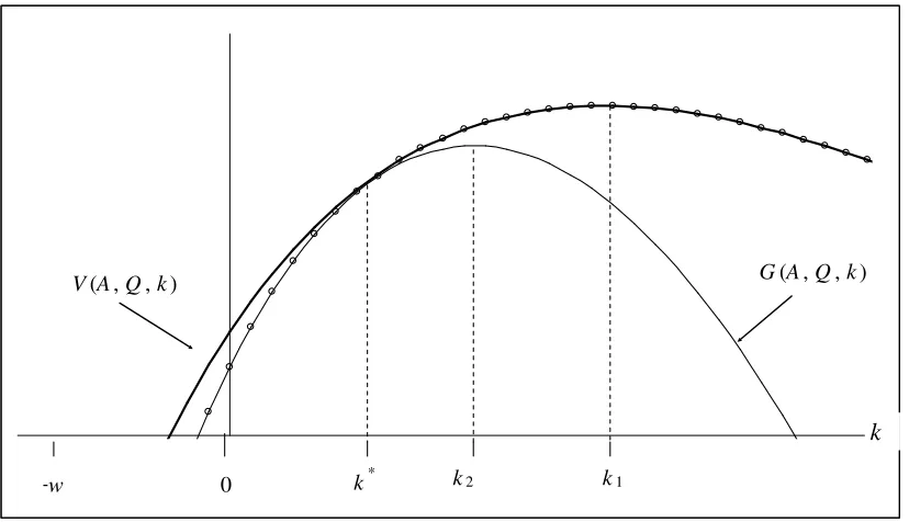
The line marked with circles in figure 1 below presents VG(A, Q, k) in that
k
k2 k1
k* 0
-w
[image:19.595.92.506.72.310.2]V(A, Q, k) G(A, Q, k)
Figure 1: The source firm’s value, VG(A, Q, k), when < * and A/Q < P*. The Thick line shows V(A, Q, k), the thin line shows G(A, Q, k) and the circles indicates VG(A, Q, k). In this case VG(A, Q, k) is maximized at k = k1 > k* implying that the source firm sets a value of k
sufficiently high to delay immediate purchases of N by the X producers.
3.3. When < * and A/Q > P*
In that case in the range k < k*the source firm’s value, represented by G(A, Q,
k) reaches a maximum in k = k2 as follows from parts (a) and (c) of Proposition 2.
Also in that case, k1 < k* as follows from parts (b) and (c) of Proposition 1. Thus, in
the range k > k*the source firm’s value, represented now by V(A, Q, k), decreases in k.
Therefore, since V(A, Q, k*) = G(A, Q, k*), the source firm’s value reaches its
maximum in k = k2.
The line marked with circle in figure 2 below presents VG(A, Q, k) in that
k* k2
k1
0 -w
k
V(A, Q, k)
[image:20.595.86.512.72.329.2]G(A, Q, k)
Figure 2: The source firm’s value, VG(A, Q, k), when < * and A/Q > P*. The Thick line shows V(A, Q, k), the thin line shows G(A, Q, k) and the circles indicate VG(A, Q, k). In this case VG(A, Q, k) is maximized at k = k2 < k* implying that the source sets a value of k
sufficiently low to promote immediate purchases of N by the X producers.
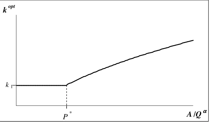
Based on the analysis of the two previous sub-sections, figure 3 below shows
the optimal k as a function of A/Q for the case when < *.
A
/
Q
ααααk
optk1
P
* [image:20.595.120.478.473.682.2]The increasing part in this function is concave and the entire function may be
below zero, as the following proposition establishes.
Proposition 3:If < t then the optimal value of k is negative.
Proof: In the appendix.
4. The optimal k in the case of a welfare objective
Assume now that the source firm is a government that is not interested in maximizing
the value of its potential sales of the resource N, namely VG(A, Q, k). Instead we
assume now that the government cares about welfare in the X market, but also want to
use it for financing its activities in other markets, markets that suffer from market
failures and government intervention in them is welfare increasing. Specifically, we
assume that the government balances these two contradicting targets by setting an
objective of bringing the value VG(A, Q, k) to a certain level M which is below the
maximal level of VG(A, Q, k). As established in section 3, in the case where < *
the function VG(A, Q, k) has an inverse-U shape and therefore there are two values of
k that yields the value M that the government seeks. For that case we assume that the
government, wishing to harm welfare in the X market as little as possible, chooses the
lower level of the two values of k that solve:
(33) VG(A, Q, k) = M
As in section 3, three cases will be analyzed next: The case where > *; The
4.1. When > *
As established in section 3.1, in this case VG(A, Q, k) is a monotonically increasing
function of k that converges to the value tAQ1 / r as k approaches infinity. In
addition it approaches - as k approaches –w, as follows from (30) and (31). Thus,
there is single value that solves (33) for every level of M that is smaller than
r
tAQ1 / .
Note that in contrast to the case where the source is maximizing the value of
its potential sales of the resource N, here the value of k that is chosen is not
necessarily infinite. The reason for that is that in the current case the source is a
government that cares not just about the revenues from selling N but also about the
welfare in the market for X. The only possibility for the government to set an
infinitely large level of k is if the M it want s to extract from the x market is above
r
tAQ1 / .
By (21), (32) and an implicitly differentiation of (33):
(34) 0
, ,
1 '
k Q A V dM
dk
K
where the inequality follows from the result that in this case VK(A, Q, k) < 0, as
established in the proof of part (a) of proposition 1. Thus, the larger the value of the
revenues that the government wants to extract from the X market the larger the level
of k it sets. In a similar manner it can be shown that in this case k is decreasing in A
and increasing in Q.
(35) V*(A,Q) V[A,Q, k*(A, Q )] = G[A,Q, k*(A, Q )]
where k* is a function of A and Q by (8). Applying (8) in (21) yields V*(A, Q)
explicitly. Based on the analysis of the properties of VG(A, Q, k) in section 3.1, if M is
smaller than V*(A, Q) then the government chooses is below k*, implying an
immediate purchases of N and production of X. Otherwise, the k that the government
chooses is above k*, a choice that sends the market to a period of inaction until A is
sufficiently large so that P = PH.
4.2. When < * and A/Q < P*
Based on figure 1 and the analysis in section 3.2, in this case VG(A, Q, k) has
an inverse-U shape maximized at k = k1 > k*. In the range –w < k < k* the function
VG(A, Q, k) is based on G(A, Q, k) and for higher levels of k it is based on V(A, Q, k).
The value of VG(A,Q, k) at its maximum satisfies:
(36) V1(A,Q) V[A,Q, k1(A, Q )].
Note that k1 is a function of A and Q by (24). Applying (24) in (21) explicitly yields
V1(A, Q), which is the maximal level of M that the government can extract form the
market in this case. If the government is interested in a level of M that is satisfying:
V*(A, Q) < M V1(A, Q) then the level of k that the government chooses, based on
(33), is above k*, implying inaction until A is sufficiently large so that P = PH. If, on
government chooses a value of k that is smaller than k*, implying immediate
purchases of N and construction of X.
An important difference from the case where the source maximizes the value
of VG(A, Q, k), is that in that case the value of k was constant at k1 whereas here it is
increasing in Q and decreasing in A.
4.3. When < * and A/Q > P*
Based on figure 2 and the analysis in section 3.3, in this case VG(A, Q, k) has
an inverse-U shape maximized at k = k2 < k*. In the range –w < k < k* the function
VG(A, Q, k) is based on G(A, Q, k) and for higher levels of k it is based on V(A, Q, k).
The value of VG(A,Q, k) at its maximum satisfies:
(37) G2(A,Q) G[A,Q, k2(A, Q )]
where k2 is function of A and Q by proposition 2.
G2(A, Q) is the maximal level of M that the government can extract form the
market in this case. If the government is interested in a level of M that is G2(A, Q)
then the level of k that the government chooses, based on (33), satisfies k < k2 < k*,
implying an immediate purchases of N and construction of X.
As in the case where the source maximizes the value of VG(A, Q, k), the value
of k that the government chooses is increasing in Q and decreasing in A.
References
Dixit, Avinash. 1989. “Entry and Exit Decisions under Uncertainty.” Journal of
Dixit, Avinash. 1991. “A Simplified Treatment of the Theory of Optimal Regulation
of Brownian-Motion.” Journal of Economic Dynamics and Control 15:
657-673.
Leahy, John V. 1993. “Investment in Competitive Equilibrium: The Optimality of
Myopic Behavior.” Quarterly Journal of Economics (November): 1105-1133.
Appendix
A. Establishing condition (17)
In this appendix we derive the benchmark condition (17) for the value of the source
firm at the time instants in which P hits PH. For that end we use the discrete
approximation of a Brownian Motion presented in Dixit (1991). Since it is more
convenient to perform this approximation for a Brownian Motion, rather than to a
Geometric Brownian Motion, the analysis is based on the function:
(A.1 ) F(a, Q, k) V(A, Q, k)
where a lnA. Due to this definition, to prove that By Itô’s lemma, a is a Brownian
Motion since A is a Geometric Brownian Motion. The drift and variance parameters
of a are denoted here by a and a2. To approximate the motion of a we divide time to
small intervals of length
(
and the variable a space into steps of size)
. The variable anow ranges over a discrete set of values ai such that:
Starting at state ai, time
(
later the variable a takes with probability p a stepdown to the value of ai-1, or takes with probability q = 1 – p a step up to the value of
ai+1. Two conditions relating
(
,)
, p and q to a and a should be used in order tomake this process an approximation of the original Brownian Motion. First:
(A.3)
(
= q)
+ p(-)
),which leads to:
(A.4) q =
! "
)
(
1 2 1, p =
! "
)
(
1 2 1The condition regarding the variance of the process is:
( A.5) 2
(
= q()
-(
)2 + p(-)
-(
)2 =)
2 + 2()
(p – q) + ((
)2 =)
2 - 2(
2eliminating the term with
(
2 leaves:(A.6) 2
(
=)
2When P = Q
A
is at the investment threshold PH then, by (1):
(A.7)
1 1
! "
! "
H a
H P
e
P A Q
if time
(
later a takes a step up the endogenous investment by the X producers raises Qsuch that P remains at PH, this implies that Q is raised to the level:
(A.8) ...
6 1 2 1 1 3 3 1 2 2 1 1 1 1 ! " ! " ! " ! " !
" ) )
) ) H a H a H a H a H a P e P e P e P e P e i i i i i
The change in Q during that time is therefore:
(A.9) )
) 1 1 1
! " ! " ! " * H a H a H a P e P e P e Q i i i
+ o(
)
),where o(
)
) collects all the terms that go to zero faster than)
, such that o()
)/)
0 as)
0. Note from (A.6) that(
too falls under the category of o()
).The Bellman equation for the value of the source when ai and Q are such that
P = PH is:
(A.10) F(ai, Q, k) = tPHQ
(
+ e-r([pF(ai-1, Q, k) + qF(ai+1, Q + *Q, k) + qk*Q](A.10) shows the value of the source in that situation as the sum of the immediate tax
revenue and the time
(
later value of the source discounted by e-r(. With probability pthe variable a takes a step down and the source's value becomes F(ai-1, Q, k). With
probability q the variable a takes a step up. In that case endogenous firm's investment
raises Q by *Q and the source's value becomes F(ai+1, Q + *Q, k). In addition, in that
case the source also gains k*Q from sales to the X producers.
(A.11) e-r( = 1 + (-r
(
) + ... 62
3
2
(
(
rr
= 1 + o(
)
)Applying this in (A.10) and expanding terms of (A.10) to Taylor series yields:
(A.12) F(ai, Q, k) = tPHQ
(
+ p[F(ai, Q, k) + Fa(ai, Q, k)(-)
) + o()
)]+q[F(ai, Q, k) + Fa(ai, Q, k)(
)
) + FQ(ai, Q, k)*Q + o()
)+ k*Q]Using p + q = 1 and the result that
(
is o()
) by itself helps simplify (A.12) to:(A.13) 0 = (q – p)Fa(ai, Q, k)
)
+q FQ(ai, Q, k)*Q + qk*Q + o()
)By (A.4), (q – p)
)
=(
= o()
) which simplifies (A.13) into:(A.14) 0 = FQ(ai, Q, k)*Q + k*Q + o(
)
)Dividing by *Q and applying (A.9) yields:
(A.15 ) FQ(ai, Q, k) = -k -
) ) )
o P
e o
H ai
By the definition of o(
)
), as)
0 the second addendum on the RHS of (A.15)approaches 0 as well. This, together with FQ(a, Q, k) VQ(A, Q, k), which follows
from the definition of F(ai, Q, k) in (A.1 ), concludes establishing (17).
B. Proof of Proposition 2
By (30) the first order condition for a maximum is
(B.1) Gk(A, Q, k) = - Q + CA1/ f ’(k) = 0,
and by (31.b):
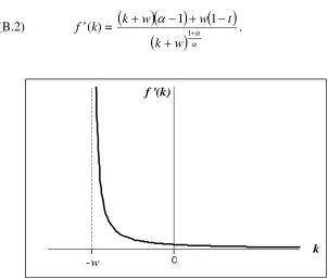
(B.2) f ’(k) =
1
1 1
w k
t w w
k
[image:29.595.92.394.344.601.2].
Figure 4:f ’(k) when > 1.
When > 1 straightforward differentiation shows that f ’(k) > 0, f ”(k) < 0, and
f ’”(k) > 0 in all of the range in which f(k) is defined, the range -w < k. In addition f(k)
approaches infinity when k approaches –w and approaches 0 when k goes to infinity.
Thus there exists a single value of k for which f ’(k) equals the positive value Q/CA1/ k
f '(k)
and for which, therefore, (B.1) holds. Since f ”(k) < 0 throughout the definition range
this k brings G(A, Q, k) to a maximum. Figure 4 shows f ’(k) in that case.
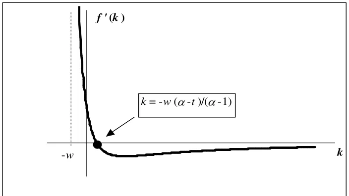
When < 1 the function f ’(k) > 0 only in the range -w < k < -w( - t)/( - 1).
In addition, in that range f ”(k) < 0, and f ’”(k) > 0 , as straightforward differentiation
shows, and f ’(k) approaches infinity when k approaches –w. Thus, in that case too,
there exists a single value of k for which f ’(k) = Q/CA1/ and (B.1) holds. Since this
value of k is in the where f ”(k) < 0 it brings G(A, Q, k) to a maximum. Figure 5
[image:30.595.113.465.302.500.2]shows f ’(k) in that case.
Figure 5:f ’(k) when < 1.
(b). Rearranging (B.1) yields that the value of k in the maximum point, k2, satisfies:
(B.3) 2
1
'
1 f k
Q A C
! "
.
(B.3) defines k2 as an implicit function of A/Q . By implicit differentiation of (B.3):
k f '(k)
-w
(B.4) 2 1 2 2 2 " 1 " ' k f Q A C k f Q A k f Q A k ! " ! " ! " + + > 0,
where the second equality follows from (B.3) and the inequality sign follows from
f”(k2) < 0, as shown in the proof of part (a). Concavity of k2 in A/Q follows from:
(B.4) 2 2
2 ! " + + Q A k = 3 2 1 2 2 2 2 2 2 1 " ' " " 1 k f Q A C k f k f Q A C ! " ! " < 0,
where the inequality sign follows from f ”(k2) < 0 and f ’”(k2) > 0 which were
established in the proof of part (a).
(c). Applying (8) and (B.2) in (B.3) shows that k2 = k* iff A/Q = P*. Yet, iff > *
then k2 > k* for all values of A/Q , as the following analysis shows. (B.4) can be
presented as: (B.5) ! " + + Q A k2 = 1 1 1 2 2 1 2 t w w k C w k Q A w k .
From (B.2) and (B.3) it follows that when A/Q approaches zero, f ‘(k) goes to
infinity implying that k approaches –w. Thus, by Lhopital’s rule, as A/Q approaches
(B.6) 0 /Q A Lim ! " + + Q A k2 = w k Lim 2 , -. $ % & w k t w w k C 2
2 1 1
1
= .
Note from (8) that when A/Q approaches zero k* approaches –w, just the same
as k2. Also note from (8) that k* is a linear function of A/Q . Thus, k2 > k* at least for
sufficiently small values of A/Q .
From (B.2) and (B.3) it follows that when A/Q goes to infinity, f ’(k2)
approaches zero. If < 1 this implies that k2 goes to -w( - t)/( - 1) and that f ”(k2) is
finite. Thus, by (B.4) the slope of k2 as a function of A/Q approaches zero as A/Q
goes to infinity. Therefore, for the case of < 1 it holds that k2 < k* iff A/Q > P*,
since by part (a) of this proposition k2 is a concave function of A/Q .
In the case where > 1 as f ’(k) approaches zero, k2 goes to infinity and f ”(k2)
goes to zero. An analysis similar to the one that leads to (B.6) yields that:
(B.7) Q A Lim / ! " + + Q A k2 = 2 k Lim , -. $ % & w k t w w k C 2
2 1 1
1
=
= [C( -1)] =
! " ! " r t t 1 1 1 1 1 .
If > * than
t
1 1 1
> 1, implying that the slope of k2 as a function of
A/Q approaches, as A/Q goes to , the slope of k* as a function of A/Q . In that case
infinitythe slope of k2 as a function of A/Q is below the slope of k* as a function of
A/Q . In that case it holds that k2 < k* iff A/Q > P*, exactly as in the case of < 1.
C. Proof of Proposition 3
If < t then < *, implying that the source firm’s value is maximized either by k1 or
by k2, depending on whether A/Q > P* or not. As shall be shown now, in that case
both k1 and k2 are negative.
To prove that k1 < 0 in that case, note that if < t then is also smaller then 1.
Thus, if < t the denominator of k1 is always positive since it satisfies:
(C.1) 1 1 t 1 t ' 1 1 t '0.
Next, note that if < t the numerator of k1 is negative since it satisfies:
(C.2) 1 – t – (1 - )t < 1 - t - (1 - t) = (1 - t)(1 - ) < 0,
since we also assume > 1/ .
To prove that k2 < 0 when < t, note once again that in that case is below
unity. As was shown in part (a) of Proposition 2,if < 1 then k2 < -w( - t)/( - 1)
leading to k2 < 0.