New Theory of Superconductivity Method of Equilibrium Density Matrix Magnetic Field in Superconductor

(1)

How to cite this paper: Bondarev, B.V. (2015) New Theory of Superconductivity. Method of Equilibrium Density Matrix. Magnetic Field in Superconductor. Open Access Library Journal, 2: e2149. http://dx.doi.org/10.4236/oalib.1102149

New Theory of Superconductivity.

Method of Equilibrium Density Matrix.

Magnetic Field in Superconductor

Boris V. Bondarev

Moscow Aviation Institute, Moscow, Russia

Received 26 November 2015; accepted 12 December 2015; published 17 December 2015

This work is licensed under the Creative Commons Attribution International License (CC BY).

http://creativecommons.org/licenses/by/4.0/

Abstract

A new variational method has been proposed for studying the equilibrium states of the interacting particle system to have been statistically described by using the density matrix. This method is used for describing conductivity electrons and their behavior in metals. The electron energy has been expressed by means of the density matrix. The interaction energy of two εkk’ electrons

de-pendent on their wave vectors k and k’ has been found. Energy εk k’ has two summands. The first

energy I summand depends on the wave vectors to be equal in magnitude and opposite in direc-tion. This summand describes the repulsion between electrons. Another energy I summand de-scribes the attraction between the electrons of equal wave vectors. Thus, the equation of wave-vector electron distribution function has been obtained by using the variational method. Particu-lar solutions of the equations have been found. It has been demonstrated that the electron distri-bution function exhibits some previously unknown features at low temperatures. Repulsion of the wave vectors k and −k electrons results in anisotropy of the distribution function. This matter points to the electron superconductivity. Those electrons to have equal wave vectors are attracted thus producing pairs and creating an energy gap. It is considered the influence of magnetic field on the superconductor. This explains the phenomenon of Meissner and Ochsenfeld.

Keywords

Density Matrix, Hamiltonian Model, Electron Distribution, Anisotropy, Electron Interaction, Superconductivity, Energy Gap, Magnetic Field in Superconductivity

Subject Areas: Computational Physics, Theoretical Physics

1. Introduction

(2)

OALibJ | DOI:10.4236/oalib.1102149 2 December 2015 | Volume 2 | e2149

While investigating dependence of Hg resistance on temperature, he could find that when the material is cooled down to about 4K temperature the resistance drops abruptly to zero. The very phenomenon was called super-conductivity. Shortly thereafter, other elements exhibiting similar properties were discovered.

A superconductor is immersed in liquid helium. Initially, weak current is supplied. Then, temperature is re-duced. When temperature falls below the defined value, the superconductor circuit is shorted. The superconduc-tor circuit current sustains its steady state as long as it can. A magnetic needle provided as a detecsuperconduc-tor finds some persistent current in the superconductor, thus indicating the magnetic field produced in the solenoid. Tempera-ture Tc, below of which a test piece exhibits its superconducting properties, is called critical temperature.

Shortly thereafter, it was discovered that such superconductivity disappears when a test piece is placed in a relatively weak magnetic field. This phenomenon was discovered by Meissner and Ochsenfeld [2]. Value Hc of

the magnetic field in which superconductivity disrupts is called a critical field. Super conductivity continuity disruption is caused by the substance-flowing current that exceeds a particular critical value (Selsby effect). Type-I and type-II superconductors of different properties have been discovered [3]. There are some other experimental superconductivity factors subjected to this description.

Superconductivity was theoretically explained by using the phenomenological expression of the Ginszburg- Landau theory [4] and forty-six years later, upon discovery of the superconductivity phenomenon by Kamer-lingh-Onnes, the microscopic theory of this phenomenon was framed by Bardeen, Cooper, and Schriffer [5]. However, many years after my student time, I cannot still understand by what means electrons are distributed over wave vectors k, when the substance superconductivity occurs and where the attraction is coming from with the electrons travelling at equal speeds.

The answer provided is rather simple by its nature. The matter of concern is a density matrix. Electrons are the very particles that make for superconductivity. As for electrons, they are classified as Fermi particles, in other words, defined by the antisymmetric functions. There are pure and mixed states specified by the quantum mechanics. Pure states are defined by the wave functions and mixed states—by the density matrix. When the quantum mechanical system is thermally coupled with a thermostat, the only correct statistical description of the system under analysis is to be considered the density matrix [6]-[13]. Kinetic density matrix equations, as appli-cable to superconductivity properties, are described in the author’s papers [14]-[25].

Complete statistical description of the system consisting of the N identical particles is provided in the quan-tum mechanics by statistical operator ρˆ( )N to satisfy the normalizing condition as follows:

( )

1 ˆ !

N

N N

Tr_ ρ = (1.1) This operator can be used for making the hierarchical sequence of operators ρ ρˆ( )1,ˆ( )2, defined by the fol-lowing relation:

( )

(

)

1 ( )

1

ˆ ˆ ,

!

n N

Tr N n

ρ = ₋ + ρ (1.2)

where n=1, 2,,N−1. In spite of the fact that statistical operators of the lowest order provide short descrip-tion of the multi-particle system, only, they are indispensible for their simplicity, particularly when some useful formulae and expressions are virtually required. This kind of a short description makes it possible to express all observable physical quantities that characterize the macroscopic system state exactly or approximately by using operators ρˆ( )1 and ρˆ( )2 , or one-particle operator ρˆ( )1, only. The one-particle statistical operator can be found by the following formula:

( )

(

)

( )

1

2 1

ˆ ˆ .

1 !

N N

Tr N

ρ = ρ

−  (1.3)

The one-particle matrix exposed to particular α-representation can be formulated as follows:

( )1 *

_{( )}

( )1

_{( )}

ˆ d

q q q

αα α α

ρ ′=

∫

ϕ ρ ϕ′ (1.4) where ϕ_α

( )

q is the wave function; α is the quantum number system under which the state of one particle is specified; q≡

{ }

r,σ , r is the particle radius vector, σ is the spin variable.

(3)

tak-OALibJ | DOI:10.4236/oalib.1102149 3 December 2015 | Volume 2 | e2149

ing into account the properties of some thermodynamic quantities to possess an extreme value when the multi- particular system is in the static equilibrium state. The equation for the wave vector electron distribution func-tion can be solved hereunder by using the variafunc-tional method.

2. Internal Fermion System Energy

The system consisting of N-identical Fermi particles can be shortly described by using one- and two-particle density matrixes:

( ) ( )

1 2 1 2

2 1

11 αα, 12,1 2 α α α α; ,

ρ ′=ρ ′ ρ ′ ′=ρ ′ ′ (2.1) One-particle density matrix ρ11′ satisfies the following normalizing condition:

, N

αα αρ =

∑

(2.2) where ρ_αα is the probability of filling the state α.

The exact expression of the internal energy of the identical particle system can be written by using the density matrix (2.1) as follows:

11 1 1 12,1 2 1 2 ,12 11 12,1 2

1

. 2

E=

∑

′H ′ρ′ +

∑

′ ′H ′ ′ρ′ ′ (2.3) Here H11′ and H12,1 2′ ′ are matrix elements of one-particle Hamiltonian

( )1 ˆ

H and the Hamiltonian Hˆ( )2 of the interaction of two particles, respectively:

1 1 1 2 1 2

11 , 12,1 2 ; .

H ′ =Hα α′ H ′ ′=Hα α α α′ ′ (2.4)

Density matrix ρ12,1 2′ ′ is antisymmetric, that is:

12,1 2 21,1 2 12,2 1 21,2 1.

ρ ′ ′=−ρ ′ ′=−ρ ′ ′ =ρ ′ ′ (2.5) Consequently, matrix elements H12,1 2′ ′ subject to the above expression (2.3), we also consider antisymmetric, that is:

12,1 2 21,1 2 12,2 1 21,2 1.

H ′ ′=−H ′ ′=−H ′ ′ =H ′ ′ (2.6) The transition from the coordinate representation, in which Hamiltonians are usually defined, to particular

α-representation is performed using the orthonormal system of wave functions ϕα

( )

q . As referred to these

functions, the matrix elements of the Hamiltonians (2.4) can be calculated by using well-known formulae as follows:

( )1 * _ˆ

d ,

H_αα′ =

∫

ϕ_αH ϕ_α′ q (2.7) ( )2

*

12,1 2 12 ˆ 1 2d d ,1 2

H ′ ′= Φ

∫

H Φ′ ′ q q (2.8)

where the integral symbol points out integration over the coordinates and indicates summation over the spin va-riable; Φ12 is a Slater two-particle wave function:

( ) ( )

{

1 2 1 2

}

12 1 2 2 1

1

. 2 ϕα q ϕα q ϕα q ϕα q

Φ = − (2.9)

Substituting this function into formula (2.8), we obtain the following antisymmetric matrix:

(

)

12,1 2 12,1 2 21,1 2 12,2 1 21,2 1 1

, 4

H ′ ′= V ′ ′−V ′ ′−V ′ ′+V ′ ′ (2.10) where

( ) ( ) (

) ( ) ( )

1 2 1 2

* *

12,1 2 1 2 1, 2 1 2 d d ;1 2

V ′ ′=

∫

ϕ_α q ϕ_α q U q q ϕ_α′ q ϕ_α′ q q q (2.11)

(

1, 2

)

U q q is the potential energy of interaction between two fermions.

(4)

12,1 2 11 22 12 21.

ρ ′ ′=ρ ρ′ ′−ρ ρ′ ′ (2.12) Substituting this expression into formula (2.3), we can formulate the following expression:

11 1 1 12,1 2 1 1 2 2 11 12,1 2

E=

∑

′H ′ρ′ +

∑

′ ′H ′ ′ρ ρ′ ′ (2.13) that meets the medium field approximation.

3. Entropy

There is a representation in which the single-party density matrix is diagonal, i.e. it has the form as follows: ,

nn wn nn

ρ ′= δ ′ (3.1) where n is a set of quantum numbers, which determines the state of one particle under the new representation;

n

w are the diagonal elements of the density matrix; δnn′ is a Kronecker symbol. By definition, value wn

points to the probability of occupation of state n by one of the particles. Thus, the function wn describes the

distribution of particles over states and satisfies the normalization condition as follows:

. n nw =N

∑

(3.2) Transition from n-representation to α-representation that specifies the matrix elements (2.4) of Hamiltonians

( )1 ˆ

H and Hˆ( )2 is performed by using a unitary transformation approach: *

,

n n n

nU w U

αα α α

ρ ′=

∑

′ (3.3) where Uαn is the unitary matrix;

*

.

n n nn

U U_α _α α ′ =δ ′

∑

(3.4) Using the distribution function wn we can write down the well-known approximated expression for the

en-tropy of the fermion system:

(

) (

)

{

ln 1 ln 1

}

.

B n n n n n

S= −k

∑

w w + −w −w (3.5)

4. Variational Principle

Referring to formulae (2.13), and (3.5), we can state that free energy F= −E ST , subject to the assumed ap-proximation, is the wn and Uαn dependent functional. Since the equilibrium state of the system corresponds to

the minimum free energy value at fixed temperature T and volume V, functions wn and Uαn can be found by

minimizing the free energy subject to conditions (3.2) and (3.4). By this means, we encounter the problem of the conditional extremum solved by employing the following auxiliary Langrange-method functional:

*

,

n n nn n

n nn

E ST µ w ′ αUαν ′Uα′

Ω = − −

∑

−

∑ ∑

(4.1)

where μ and νnn′ are undetermined multipliers. Extremum conditions for the functional where μ and νnn′ are

undetermined multipliers. Extremum conditions for the functional

*

0, 0;

n n

w U_α

∂Ω ∂ = ∂Ω ∂ = (4.2) lead to the following distribution function wn and unitary matrix Uαn equations:

(

)

ln1 n ,

n n

w

w β ε µ

−

= − (4.3)

( )eff _,

n n n nn n

w

∑

_α′H_αα′U_α′ =

∑

′ν ′U_α ′ (4.4) where εn is the mean energy of one particle:

, n n n nnwn

ε =ε +

∑

′ε ′ ′ (4.5) *

,

n α αU Hαn ααUαn

(5)

is the kinetic energy of a particle,

1

1 2 2

* * 12,1 2 1,2;1 2

2 , ;

nn UαnUαnH UαnUαn nn n n

ε ′=

∑

′ ′ ′ ′ ′ ′ ′ ′ ε ′ =ε ′ (4.7)

( )eff

Hαα ′ is the effective one-particle Hamiltonian as defined in the mean-field approximation:

( )

1, 1 11

1,1

2 .

eff

H_αα′ =H_αα′+

∑

′H_{αα α α}′ ′ρ_{α α}′

The solution is significantly easier in the case when the properties of the system under analysis make it possi-ble to predict what representation is used to bring the density matrix to its diagonal pattern. As applies to this case, it is time to solve the Equation (4.3). Any solutions sourced from the above equation can exhibit certain interesting features related to its nonlinearity and particular dependence of kernel εnn′ on quantum numbers n

and n′. The aim of this chapter is to study such features and their physical effect.

5. Statistical Description of the Electrons in the Crystal Lattice

The arrangement of atoms within a given type of crystal can be described in terms of the Bravais lattice with lo-cation of the atoms in an isolated unit cell specified. We shall determine position of one of the atoms in the unit cell using vector R and arrangement of all other atoms in the cell relative to the first one—using vector a. Let s

be a set of quantum numbers defining the wave function of one of the states of an electron located within the neighborhood of the atom, the position of which is determined by vector R + a. By using the available notations, we write the orthonormal system of wave functions that define localized electron states in the form as follows:

( )

q

(

, ,s

)

,

α

ϕ ≡ϕ r− −R aσ a

where α=

{

R a, ,s

}

is a set of quantum numbers that determine the state of the electron in the crystal lattice. In this case, the Vanier functions are preferable to use for these functions. Using these functions, we can calculate the matrix element of the Hamiltonians (2.7) and (2.8).

Using the method proposed in the previous section, the density matrix of equilibrium state of the system of electrons within a crystal can be found. Some of the simplest types of Hamiltonians only that simulate interac-tion and behavior of conducinterac-tion electrons in real metals to the extent of a particular precision will be analyzed in this chapter.

We consider the cases when one atom (a = 0) only is in the unit cell and assume that the valence electron ma-trixes (2.7) and (2.11) have the form as follows:

1

1 2 2 11 2 2

12,1 2 , ,

;

ss s s s s

H_αα_′ =ε_{R R}₋ _′δ _′ V _{′ ′}=V_{R R} _{R R}_{′ ′}δ δ_′ _′ (5.1) where parameter s takes on finite number G of different values;

( ) (

) (

) ( ) (

)

1 2, 1 2 1 1 1 1 1 2 1 2 2 2 2 2 d d ,1 2

VR R R R′ ′ =

∫

ϕ r ϕ r +R −R′ U r − +r R −R ϕ r ϕ r +R −R′ r r (5.2)

(

)

ϕ r−R is the averaged wave function that defines an electron located within the neighborhood of site R;

(

1– 2

)

U r r is the potential Coulomb-based two electron repulsion energy. In this case, the density matrix de-scribing conduction electrons is expressed as follows:

. ss

ss

αα

ρ ρ ′ ρ δ

′ ≡ RR′= RR′ ′ (5.3)

Using formulae (5.1), (5.3) and making some simple transformations, the electron energy (2.13) can be ex-pressed as follows:

{ }

{

1 2, 1 2 11 2 2

}

,

E=G

∑

RR′εR R− ′ρR R′ +

∑

R HR R R R′ ′ρR R′ ρR R′ (5.4)

where

{ }

R =R R R R₁, ₂, ₁′ ′, ₂;

(

)

1 2, 1, 2 1 2, 1, 2 2 1, 2, 1 2 1, 1, 2 1 2, 2, 1

1 4

HR R R R′ ′ = _G VR R R R′ ′ +VR R R′ R′ −VR R R R′ ′ −VR R R′ R′_ . (5.5)

(6)

( )

1

ei ,

L

w N

ρ − ′

′ =

∑

k R R

RR k k (5.6)

where the summation is performed by using vectors k of the first Brillouin zone; NL is number of lattice sites;

wk is a wave vector electron distribution function that satisfies the following normalizing condition:

1

or ;

L

G w N w

N ν

= =

∑

k k

∑

k k (5.7)

v is the extent to which the zone is filled: v=N G NL.

With the expression (5.6) substituted in the formula (5.4), the following expression can be obtained: ,

1

, 2

E G ε w ′ε ′w w′

 

= _ + _



∑

k k k

∑

k k kk k k  (5.8)

where εk is the kinetic electron energy:

ei

ε ₌

_∑

ε −kR

k R R ;

εkk′ is the energy of interaction of two electrons with wave vectors k and k′:

(

)

(

)

{ } 1 2, 1 2 1 1 2 2

2 ,

2

exp .

L

H i i

N

ε_kk_′=

∑

_{R R} _{R R}_{′ ′} _ ′− + ′ ′− _

R k R R k R R (5.9)

The equality (5.6) is, in its essence, the unitary transformation that diagonalizes the density matrix. In this case, the formula (3.5) takes on the form as follows:

(

) (

)

{

ln 1 ln 1

}

B

S= −Gk

∑

_k w_k w_k+ −w_k −w_k

While minimizing free energy subject to the normalizing condition (5.7), we can obtain the equation that makes it possible to find the wave vector conduction electron distribution function wk that is of similar nature

as the Equation (4.3):

(

)

1

ln w ,

w β ε µ

− = − k k k (5.10) where εk is the mean energy of one electron with wave vector k:

. w

εk=εk+

∑

k′εkk′ k′ (5.11)

Now, we can refer to the formula (5.9) to determine the structure of the kernel εkk′ in the functionals (5.8) and (5.11). Since diagonal elements are the greatest ones of the matrix elements (5.9), as complies with R1′ =R 1 and R2′ =R2, we can use an approximated formula as follows:

( )

₍

₎

1 21 2 1 2 11 2 2 1 2

0

1 1 2 2 ,

VR R R R′ ′ =UR−RδR R′δR R′ +UR−Rδ R −R′−R +R′ (5.12)

where

1 2

UR−R is the mean energy of Coulomb interaction of two electrons localized at the sites R1−R2 and the second summand approximates the off-diagonal elements. In the strict sense, the function U(0) in the formula (5.12) should depend not only on R1−R2, but also on R1−R1′. Using formulae (5.5), (5.8), (5.9), and (5.12) we obtain the following approximate expression for interaction energy of electrons:

(

)

int 0 , 1

, 2

E = G vU N−

∑

k k′Jk k− ′w wk k′+

∑

kI w wk k −k (5.13)

where

( )

1

ei ;

L J U N ′ − ′ − =

∑

k k R

k k R R (5.14) ( )0

(

2

)

e i ;

Ik =

∑

RUR G− − kR (5.15)

(7)

does not depend on the distribution function wk. The following summand represents the exchange energy of

electrons. The kernel Jk k− ′ in the above sum is a positive function that takes on the largest value at k′ = −k and rapidly decreases against increase of the

[

k′ −k

]

as a result of long-range Coulomb interaction behavior. Since the exchange energy is negative, such behavior of the function Jk k− ′ makes for effective attraction to occur between electrons with the nearest wave vector values. As applies to the positive summands expressed in the formula (5.13) that contain values Ik, they simulate effective repulsion of k and –k wave vector electrons.

The mean one-electron energy (5.11) that corresponds to the interaction energy (5.13) can be formulated as fol-lows:

,

J w I w

εk =εk−

∑

k′ k k−′ k′+ k −k (5.16)

Unfortunately, while using the formula (5.14) or (5.15), it is impossible not only to find any analytical solu-tion of the Equasolu-tion (5.10), but also to study it in details. Therefore, we approximate the funcsolu-tion (5.14) by using the following expression:

,

Jk k− ′ =Jδkk′

where J is a positive constant; and the value (5.15) can be considered as that does not depend on a wave vector: .

Ik=I

As applies to this case, the formula (5.16) takes on the following expression:

Jw Iw

εk =εk− k+ ₋k (5.17)

and the energy of two electron interaction with wave vectors k and k′ takes on the following expression: .

J I

ε_kk_′= − δ_{k k}₋_′+ δ_{k k}₊ _′ (5.18)

6. Electron Wave Vector Distribution Function

The formula (5.17) can be used for transforming the Equation (5.10) as follows:

(

)

1

ln w Iw Jw .

w β ε − µ

−

= + − −

k

k k k

k

(6.1) In this equation, we substitute k for −k. Since ε−k=εk, we can obtain the following expression:

(

)

1

ln w Iw Jw .

w β ε µ

− − − − = + − − k

k k k

k

(6.2) Equations (6.1) and (6.2) result in the following combined equations for two values wk and w−k of the

electron distribution function:

(

)

(

)

1 ln , 1 ln . w Iw Jw w w Iw Jw w

β ε µ

− − − − − ₌ ₊ ₋ ₋     − _ = + − −  k

k k k

k k

k k k

k

(6.3)

We can demonstrate that this system admits two types of solutions. One of them describes isotropic wave vectors distribution of electrons and other—anisotropic wave vectors distribution of electrons. If

w−k=wk (6.4)

then each of the Equation (6.3) transformed can be formulated as follows:

(

)

(

)

1

ln w I J w .

w β ε µ

− = + − − k k k k (6.5) If I = J, this equation is solvable as the Fermi-Dirac function.

The unknown functions wk and w−k, expressed via Equation (6.3), admit as combined functions where the

kinetic electron energy εk acts as a intervening variable: w−k =w1

( )

εk and wk =w2

( )

εk . The functions

( )

1 1

(8)

(

)

(

)

(

)

(

)

(

)

(

)

1

2 1

1

2

1 2

2

1 2

ln 2 1 1 ,

1 2

ln 2 1 1 .

w

f w f w

w

f w f w

w

τ

− ₌ _{+ −} _{− +} 

 

− _

= + − − +





(6.6)

where

4

, ,

J I J I

ε µ− _τ θ

= =

+ +

 (6.7) energy ratio I and J defined by the parameter

.

J I

f

J I

− =

+ (6.8)

In this chapter, we will study the case when the parameter J = 3I; in this case f = 1/2.

7. Anisotropy

We have prescribed function f = f(a), i.e. value f depends on vector a. If value f depends on modulus of this vector a,only, the distribution concerned is called isotropic, i.e. it may be formulated as f = f(a). We will depict a sphere of radius a centered in the origin of coordinates. So, value f will remain equal at any point of this sphere, providing that f = f(a) is the isotropic function. Any other f = f(a) function will be referred to the anisotropyone.

Now, we will consider the example of the anisotropic function. We will depict two vectors. One of them will be an arbitrary vector a and the other one will be rated as equal, but opposite in its direction −a. So, if it is ap-peared that function values fail matching in the points concerned, i.e.

( )

,

f a ≠ f −a (7.1) this function will be called the anisotropic one.

8. Isotropic Distribution of Electrons

We express the combined Equation (6.6) regarding the case when no anisotropic condition is available, i.e. w1 =

w2 = w0. Now we can obtain the following equation:

(

)

0

0 0

1 4

ln w fw .

w τ

−

[image:8.595.176.455.522.692.2]

= _− (8.1) This function is graphically represented in Figure 1.

Figure 1.Isotropic energy distribution of electrons regarding the case when J = 3I

(9)

9. Anisotropic Distribution of Electrons

With the electrons being distributed over wave vectors in the anisotropic manner, we will introduce new va-riables d and s by means of the following relations:

2– 1 , 1 2 1 .

w w =d w +w = +s (9.1) Without loss of generality, the difference d of two values w1 and w2 of the distribution function can be consi-dered as a nonnegative value: d ≥ 0,

( )

1 2

w  ≤w  . (9.2) In this case, the largest value d equals to one: d∈

[ ]

0,1. Value s can take on those to be ranged from −1 to 1:

[

1,1

]

s∈ − . Now, we solve Equation (9.1) relative to the probabilities w1 and w2:

(

)

(

)

1 2

1 1

1 , 1 .

2 2

w = + −s d w = + +s d (9.3) Using the formulae (9.3), we transform the combined Equation (6.6). For this purpose, we at first subtract one equation from other and then sum them up. As a result, we can obtain the following combination:

(

)

(

)

(

)

(

)

(

)

2 2

4

2 2

1

e ,

1

1 1

ln 1 .

8 1 2

d

d s

s d

s f

s d

τ



+ −

= 

− − _



− − 

= + + _

+ − _



(9.4)

The first equation of the above combination is easily to solve in relation to s:

( )

(

)

2 44

(

)

2

1 e 1

e 1

d d

s d

τ

− − +

= ±

− . (9.5)

As provided by the relations (9.3) hereinabove, the probabilities w1 and w2 can be considered as the functions of parameter d: w₁=w d₁

( )

, w₂=w₂

( )

d . The second combined Equation (9.4) makes it possible to express the electron energy  by using parameter d. As based on the obtained dependencies, it is easy enough to plot the function graphs w₁=w₁

( )

 and w₂

( )

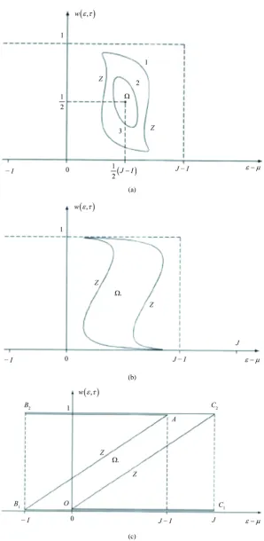
 for various temperature values. Such anisotropic curve graphs are demonstrated inFigure 2. Many-valuedness of the function w=w

( )

 proves that various equilibrium states of conduction electrons in metals are possible at the same temperature. These macro-states are different from those represented by the Bloch electron distribution function. As a matter of the fact, it is the electron minimum ener-gy macro-state that can be actually implemented provided, that this kind of state is rather stable and it is kept out of any disruption under external effects.

The plots, demonstrated in Figure 1 and Figure 2, provide a particular insight into electron state distribution pattern shaped up under various metal temperatures. When temperature τ ≥ 1, the isotropic electron wave vector distribution only is possible that is described by the function w_k =w₀

( )

ε_k . The function graph curve w₀ =w₀

( )



stated against all temperature values passes point Ω at the coordinates of ε µ= +

(

J−I

)

2 and w=0.5. When the temperature falls down (τ <1), the curve slope at this point is increased. When temperature drops down to rather low values, the dependency curve w₀=w₀

( )

 is bent so that it looks like letter Z.

A closed anisotropic curve originates at point Ω of the curve w0=w0

( )

 at τ = 1 and its dimensions increase

against the falling temperature. The curve shape also changes. The following critical temperature corresponds to value τ = 1:

. 4 c

I J

T k +

(10)

OALibJ | DOI:10.4236/oalib.1102149 10 December 2015 | Volume 2 | e2149 (a)

(b)

[image:10.595.163.462.79.691.2]

(c)

Figure 2. Anisotropic energy distribution of conduction electrons regarding the cases when: (a)

(11)

10. Electron Distribution at

T

= 0

Now, we consider the electron distribution function at T = 0 in details. Within the range of τ → 0, the isotropic distribution solvable by the Equation (8.1) is expressed as follows:

( ) (

) (

)

0

1 at ,

at ,

0 at .

J I

w J I J I

ε µ

ε ε µ µ ε µ

ε µ

≤ + − 



=_ − − ≤ ≤ + −

 _≥



(10.1)

This dependence is graphically represented in Figure 1.

Within the range of τ → 0, as stated by the Equation (9.4), the following occupation probability dependence w

of the kinetic electron energy ε that describes anisotropic electron wave vector distribution can be formulated:

( )

1 at ,

at ,

0 at .

i

I

w w I J

J

ε µ

ε ε µ ε µ

ε µ

≤ − 



=_ − ≤ ≤ +

 _{≥ +}



(10.2)

where i = 1 or 2. So, the values of functions w1=w1

( )

ε and w2=w2

( )

ε produce the following pairs:

( )

1 0 and 2 1

w ε = w ε = (10.3)

at µ− ≤ ≤ +I ε µ J, or

( ) (

)

( )

1 and 2 1

w ε = ε µ− +I J w ε = (10.4)

at µ− ≤ ≤ + −I ε µ J I, or

( )

( ) (

)

1 0 and 2

w ε = w ε = ε µ− J (10.5) at 0≤ ≤ +ε µ J.

As demonstrated in Figure 2(c), the AB1C1O polygonal line meets the relationship w1=w1

( )

ε and the

AB2C2O polygonal line—the relationship w2 =w2

( )

ε .

11. Electron Energy Calculation at

T

= 0

Now, we calculate the energy of electrons distributed isotropically or anisotropically. For this purpose, we use the normalizing condition that can be expressed by the following equation:

.

G

∑

kwk =N (11.1)

The electron system energy, when approximated in the mean field, takes on the following expression:

(

2

)

1

2 .

2

E= G

∑

k εkwk+Iw wk −k−Jwk (11.2)

As the distribution function w = w(ε) is known, we can find chemical potential and electron energy at T = 0. Such calculations are demonstrated in the previous papers [18]-[23]. In fact, it is macro-state of the electron energy minimum that can be actually implemented. The energy calculated at T = 0 is the lower-range one re-garding the condition described by the following formula:

1 at

0 at .

w

I

ε µ

≤ 

=  _{> −}



k k

k

(11.3) This function is anisotropic at µ− <I εk≤µ.

We approximate the dependence of the kinetic electron εk on the wave vector k formula

2 2 . 2m

ε =k k 

(12)

Using the relation (11.3), we obtain the normalizing condition to a symbolic equality

0 d ,

AN

G

∑

_k=

∫

∞ ε ε (11.5) where 2₂ ₃

2π

G m mV A

N

=

 , V—the crystal volume, N—the number of valence electrons. In this case, the

norma-lizing condition results in the following equation:

0 d 1,

A

∫

∞ ε ε= (11.6) and the energy follows that

0 d .

AN

E=

∫

∞ ε ε (11.8)

12. Superconducting Electron State

The distribution function is a single-valued one. This means that one value of the distribution function shall cor-respond to one value of the energy. As concerns the anisotropic distribution function, it is two-valued. It simul-taneously determines two values of the wave vectors k and −k, to which two values of the distribution function

( )

1

w₋_k =w ε_k and wk =w2

( )

εk are conformed. However, whether the values w−k=w2

( )

εk and wk =w1

( )

εk

can be conformed to the above vectors. In this case, the superconductivity phenomenon is examined.

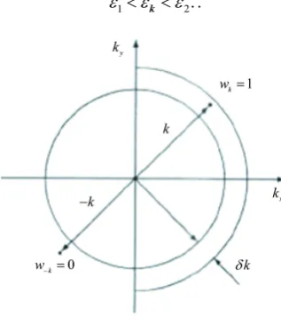
For detecting superconductivity, initially weak current is supplied to a conductor. Then, temperature is re-duced. When temperature falls below the defined value, the superconductor circuit is shorted. The superconduc-tor circuit current sustains its steady state as long as it can. Let current flows along axis x. Than at T = 0, the fol-lowing electron wave-vector space distribution function k can be represented in Figure 3.

13. Electron Mean Energy

Dependence ε ε ε=

( )

of the electron mean energy ε against kinetic energy ε can be found by the formula (5.17):

( )

(

J I w

) ( )

0 at 1, 2;

ε ε = −ε − ε ε ε ε ε≤ ≥ (13.1)

( )

Iw1

( )

Jw2

( )

at 1 2.

ε ε = +ε ε − ε ε < <ε ε (13.2) This dependence, as rated at various temperatures τ, is graphically represented inFigure 4. At T < Tc, each of

the curves ε ε ε=

( )

has a “well” conforming to values of the kinetic energy anisotropy ε, that satisfies the in-equalities as follows:

1 2.

ε <ε_k<ε . (13.3)

[image:12.595.230.389.515.694.2]

(13)

[image:13.595.189.441.80.383.2]

Figure 4. Dependence of the mean electron energy ε of the kinetic energy ε at various temperature values τ: 1: τ = 0; 2: τ = 0.75; 3:

τ = 0.95.

Value ε1 is the lower-range value of the kinetic electron energy ε subject to functions w1

( )

ε and

( )

2

w ε . Value ε2 satisfies the following condition:

( )

1

( )

2 ,

ε ε =ε ε (13.4) according to which the “well” edges, represented by the graphic chart ε ε ε=

( )

, are shown at the same level. However, there is an opening on the well edge’s right. This means that there is a certain “gap” in the spectrum of values of the electron energy ε. The energy gap width ∆ extends from zero to value J, when temperature falls down from Tc to zero. The well width

2 1

δε ε= −ε (13.5) is also extended from zero to value I at T = 0.

14. Real-Valued Distribution Function

The lower-range electron energy corresponds to the real-valued equilibrium distribution function. The real-valued equilibrium distribution function follows from the electron energy calculated for various distribution functions. The function curve, as rated against τ = 0.75, is shown inFigure 5.

15. Type-I and Type-II Superconductors

For characterizing type of a superconductor, the following parameter value is involved: .

I I J

ζ =

+ (15.1)

(14)

1 . 2

f

ζ = − (15.2) This function is graphically represented in Figure 6. Using known inequalities, we can write the supercon-ductor type condition. The condition ζ <1 2 indicates to a type-I superconductor. And the condition

1 2

ζ > indicates to a type-II superconductor. These conditions have been originally gained by A. A. Abri-kosov.

Parameter f = −1 shows that value of J = 0, that characterizes the gap width ∆, does not produce any pair.

Consequently, the coherent length ξ (i.e. electron pair interaction length) equals zero, as well. As applies to this case, the condition ξ < λ satisfies where λ is the superconductor magnetic field penetration depth. This condition shows that the type-II superconductor is in the range of the f parameter-defined values.

16. Density Matrix

Now, when we find the probability wk, it is possible in principle to find the density matrix. Using a unitary

transformation, we have

[image:14.595.173.452.282.478.2]

Figure 5.Real-valued conduction electron equilibrium distribution function at τ = 0.75. Electron interaction energy values I and J are coupled by the J = 3I relation.

[image:14.595.172.450.527.708.2]

(15)

( )

1

ei

L

w N

ρ − ′

′=

∑

k R R

RR k k . (16.1)

Unfortunately, the calculations carried out at arbitrary temperatures are very complex. The density matrix can be calculated only for the probability of (11.3) at the temperature T = 0:

( ) ( )

,0 , 0,

1 1

e e .

x

i i

I k I

L L

N ε µ N µ ε µ

ρ − ′ − ′

′=

∑

_{< < −} +

∑

_> _{− < <}

k k

k R R k R R

RR k k (16.2)

17. The Meissner and Ochsenfeld Effect

When a specimen is put in a relatively weak magnetic field superconductivity vanishes. Such phenomenon was discovered by Meissner and Ochsenfeld [2]. Magnetic field strength Hm at which superconductivity is

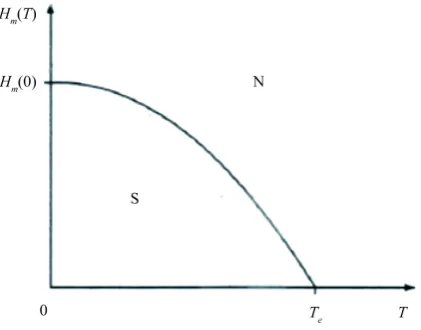
de-stroyed is known as the critical field. Temperature dependence of the critical field is described by the following empirical formula:

( )

_{0 1}

(

2

)

_,

m T m

H =H −τ (17.1) where H_m

( )

0 is the magnetic field strength at absolute zero of temperature T = 0. The dependence (17.1) is plotted inFigure 7.

The plane (H, T) is represented by a superconductive state phase diagram. Asdemonstrated inFigure 7, the substance in superconductive state S is found under the curve and that to be in normal state N—above the curve. Any superconductor introduced by such state diagram is known as the type-I superconductor. We will hereafter consider the superconductors of such type only.

18. Magnetic Field in Superconductor

With an electron having a spin, Hamiltonian Hˆ( )1 , in the presence of a magnetic field, will be expressed as fol-lows:

( )1 2 2

_{( )}

ˆ _,

2 m

H U H

m µ

∇

= − + r − (18.1) where µ µ ξ= B is a spin magnetic moment of an electron; µB=e

( )

2m is a Bohr magneton; ξ = ±1 2 is

an electron spin; U(r) is potential electron energy; Hm is magnetic field strength.

Let’s a wave function will be written as follows:

( )

q _s

(

) ( )

,

α σ

ϕ =φ r−R χ ξ (18.2) where φ_s

(

r−R

)

is a coordinate function; R is a vector defining the ion around which an electron moves;

( )

σ

[image:15.595.216.427.541.706.2]

χ ξ is a spin function; s=1, 2,,ns; α =

{

R, ,sσ

}

. Let’s assume that functions φs

( )

r are mutually

(16)

equal: φs

( ) ( )

r =φ r . Spin functions only are different. Thereafter, we will obtain two following functions:

( ) (

q

) ( )

,

α σ

ϕ =φ r−R χ ξ (18.3) In this case, matrix elements of the one-body Hamiltonian may be written by using the following expression:

( )1 * _ˆ

d .

H_αα′ =

∫

ϕ_αH ϕ_α′ q (18.4)

If we substitute formula (18.4) herein, we will obtain the following expression:

(

1 2

) (

1 2

)

( ) ( )

1 2 1 2 . 1

2

R R ss B m RR ss

H_αα′=ε − ′δ δ_σσ′ ′+ µ H δ δ′ ′χ_σ − χ_σ′ − −χ_σ χ_σ′  (18.5) Density matrix aa′ is transformed to the diagonal form by means of the following unitary matrix:

,

1

ei ,

s s ss L

U U

N

α ≡ Rσk′ ′σ = kRδ δ′ σσ′ (18.6)

where κ=

{

k, ,sσ

}

. Hence, density matrix aa′ turns to the matrix as follows:

.

ss

w

κκ′= kδ δ δkk′ ′ σσ′

 (18.7) After simple transformations we will obtain the expression of the non-interacting electron energy:

(

)

1 ,

E =G

∑

k εk− Λ wk (18.8)

where G=2ns,

1 , 4µBHS

Λ = (18.9)

( )

(

)

(

2 2

)

1 2 1 2 .

S=

∑

_σ χ_σ −χ_σ − (18.10) On adding the above formula to the energy Eint of interacting electrons, we can obtain the following elec-tron energy expression:

(

)

1

(

2

)

. 2

E=G ε − Λ w + Iw w− −Jw 

 

∑

k k k k k k (18.11)

With thermodynamic potential Ω minimized taking into account the energy (11), we will come to the follow-ing integral equation applicable for findfollow-ing the distribution function wk of wave-vector conduction electrons

when a specimen is exposed to a magnetic field:

(

)

1

ln w Jw Iw .

w β ε − µ

−

= − Λ − + −

k

k k k

k

(18.12) Let’s assume that

.

ε_k′ =ε_k− Λ (18.13) Then, the distribution function equation will take up the previous solution:

(

)

1

ln w Jw Iw .

w β ε − µ

− _′

= k− + −

k

k k

k

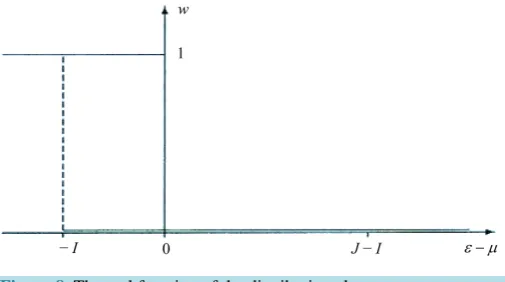
(18.14) Now, we shall consider the case when a magnetic field destroys superconductivity at T = 0. The valence elec-tron energy is herein expressed by the formula (11). If a superconductor is not exposed to a magnetic field, the real distribution function takes up the form shown in Figure 8.

Let’s assume that the magnetic field strength is expressed as follows:

(

0 ,

)

I δε τ

Λ = ≡ = (18.15)

(17)

[image:17.595.187.440.86.227.2]

Figure 8. The real function of the distribution electrons at temperature

τ = 0. The magnetic field is absent.

Figure 9. Real conduction electron energy distribution at τ = 0. As exposed to a magnetic field at which superconductivity vanishes.

With the distribution function taking up the following formula, superconductivity vanishes:

1 at ,

0 at .

w ε µ

ε µ

≤ 

= 

≥ 

k k

k

(18.16) In this case, the normalizing condition results in the following equation:

0 d 1,

A

∫

µ ε ε= (18.17) it follows that

.

F

µ ε= (18.18) The valence electron energy (18.11), wherein J = 3I and Λ= I, may be calculated by the following formula:

( )

₍

₎

0 2 d .

m

E =AN

∫

µ ε− I ε ε (18.19) As a result, we shall obtain the following expression:

( ) 3 2

. 5 m

F F I

E Nε

ε

 

= _ − _

  (18.20)

But should the superconductivity state be survived and the distribution function is expressed as follows:

1 at ,

1 at , 0;

0 at , 0;

0 at .

x

x I k

I k

I

µ

µ µ

ω

µ ε

µ µ ε

ε ε

≤ 

 _< _{< +} _> 

=  _< _{< +} _< 

 _{≥ +}



k k k

k k

[image:17.595.188.444.254.400.2]

(18)

The distribution function can be found real, if the electrons possess less energy. As for the function (18.21), the normalizing equation takes up the following form:

1 0

1

d d 1.

2

A µ A µ e

µ

ε ε+ + ε =

∫

(18.22) This equation yields the following chemical potential:

2 2 1 . 2 16 F F F I I µ ε ε ε   = _ − − + _

  (18.23)

In view of the expression formulated here in above (18.11), the electron energy may be calculated by means of the following formula:

( )

₍

₎

0

1 1 1

d d

2 2 2

I s

E =AN µ_ε− Λ − J−I _ ε ε+ AN _µµ+ _ε− Λ − J_ ε ε

   

∫

Let’s assume that J = 3I and Λ = I. Then, we will obtain the formula as follows:

( )

₍

₎

0

1 5

2 d d

2 2

I s

E =AN µ ε− I ε ε+ AN _µµ+ _ε− I_ ε ε

 

∫

(18.24)

On calculating, the formula below is obtained:

( ) 3 3 3 2

2 .

5 20 16

s F

F F

I I

E Nε

ε ε  _ _ _ _    = −_ − _ − _ _ +         (18.25) Now, we can find the energy differential:

( ) ( ) 3 5

1 0. 20 4 m s F F I

E E Nε

ε

 

− = − _ − + _<

  (18.26)

As seen, energy E( )m of state that is produced by the superconductivity-destroying magnetic field occurs to be less than energy E( )s of the superconductive state:

( ) ( )

.

m s

E <E (18.27) This means that any superconductivity exposed to a magnetic field vanishes.

19. Magnetic Field Strength

We take parameter Λ as equal to I. In this case, the distribution is displaced on its right. Now we will find the critical magnetic-field strength at T = 0:

( )

1

0 .

4µBHm S=I (19.1) If temperature τ is above zero, than the critical magnetic-field strength, as referred to the formula (9), can be formulated as follows:

( )

1

,

4µBHm τ S =δε τ (19.2) where δε τ

( )

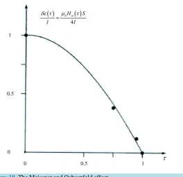
is the width of a potential well (13.5) on the average electron energy to kinetic energy curve as specified at temperature τ.

If to refer to a theoretical average electron energy to kinetic energy curve demonstrated inFigure 4, specific temperature dependence curve of the critical magnetic-field strength is plotted. Such curve is shown in Figure 10.

(19)

[image:19.595.188.453.81.337.2]

Figure 10. The Meissner and Ochsenfeld effect.

( )

1

( )

4 BHm S

δε τ = µ τ (19.3) may be used for measuring the width of an energy well.

20. Conclusions

The model for electrons in metal, described in this paper, can be assumed as a basis of an alternative theory of superconductivity. This model significantly differs from those which have been applied in the contemporary theory of superconductivity. The superconductivity, described herein, is caused by repulsion of wave vector k

and −k electrons, but electron pairs and energy gap in the spectrum—by attraction between the electrons of equal wave vectors. Electrons are statistically described in terms of the density matrix formalism, featured with the simplicity representative by specific formulae and physical content. The problem examined demonstrates advantages of the density matrix method.

In this paper we consider that critical magnetic field removes the superconductivity. It is shown that this is due to the width of the hole in the dependence of the average energy of an electron from its kinetic energy. This connection can be used for the experimental dependence of the width of the hole on the temperature.

References

[1] Kamerlingh-Onnes, H. (1911) Further Experiments with Liquid Helium. On the Change of Electric Resistance of Pure Metals at Very Low Temperatures, etc. IV. The Resistance of Pure Mercury at Helium Temperatures. Comm Phys Lab

Univ Leiden, 122, 13-15.

[2] Meissner, W. and Ochsenfeld, R. (1933) Ein neuer Effekt bei eintritt der Supraleitfähigkeit. Naturwissenschaften, 21, 787-788. http://dx.doi.org/10.1007/BF01504252

[3] Abrikosov, A.A. (1952) Современное состояние проблемы сверхпроводимости. Proceedings of Academy of

Science of the USSR, 86, 489;

Abrikosov, A.A. (1965) Современное состояние проблемы сверхпроводимости. Uspekhi Fizicheskih Nauk, 87, 125-142. http://dx.doi.org/10.3367/UFNr.0087.196509h.0125

[4] Ginszburg, V.L. and Landau, L.D. (1950) Towards the Theory of Superconductivity. Journal of Experimental and

Theoretical Physics, 20, 1064.

(20)

OALibJ | DOI:10.4236/oalib.1102149 20 December 2015 | Volume 2 | e2149 [6] Von Neumann, J. (1964) Mathematical Foundations of Quantum Mechanics. Nauka, Moscow.

[7] Shen, Y.R. (1967) Quantum Statistics of Nonlinear Optics. Physical Review, 155, 921-931.

http://dx.doi.org/10.1103/PhysRev.155.921

[8] Grover, M. and Silbey, R. (1970) Exciton-Phonon Interactions in Molecular Crystals. Journal of Chemical Physics, 52, 2099-2108. http://dx.doi.org/10.1063/1.1673263

[9] Kossakowski, A. (1972) On Quantum Statistical Mechanics of Non-Hamiltonian Systems. Reports on Mathematical

Physics, 3, 247-274. http://dx.doi.org/10.1016/0034-4877(72)90010-9

[10] Gorini, V., Kossakowski, A. and Sudarshan, E.C.G. (1976) Completely Positive Dynamical Semigroups of N-Level Systems. Journal of Mathematical Physics, 17, 821-825. http://dx.doi.org/10.1063/1.522979

[11] Lindblad, G. (1976) On the Generators of Quantum Dynamical Semigroups.Communications in Mathematical Physics,

48, 119-130. http://dx.doi.org/10.1007/BF01608499

[12] Gorini, V., Frigeio, A., Verri, N., Kossakowski, A. and Sudarshan, E.C.G. (1978) Properties of Quantum Markovian Master Equations. Reports on Mathematical Physics, 13, 149-173. http://dx.doi.org/10.1016/0034-4877(78)90050-2

[13] Blum, K. (1981) Density Matrix Theory and Application. Plenum, New York and London.

http://dx.doi.org/10.1007/978-1-4615-6808-7

[14] Bondarev, B.V. (1991) Quantum Markovian Master Equation for System of Identical Particles Interacting with a Heat Reservoir. Physica A, 176, 366-386. http://dx.doi.org/10.1016/0378-4371(91)90294-M

[15] Bondarev, B.V. (1992) Quantum Markovian Master Equation Theory of Particle Migration in a Stochastic Medium.

Physica A, 183, 159-174.http://dx.doi.org/10.1016/0378-4371(92)90183-Q

[16] Bondarev, B.V. (1992) Quantum Lattice Gas. Method of Density Matrix. Physica A, 184, 205-230.

http://dx.doi.org/10.1016/0378-4371(92)90168-P

[17] Bondarev, B.V. (1994) Derivation of Quantum Kinetic Equation from the Liouville-von Neumann Equation. Teor. Mat. Fiz., 100, 33-43.

[18] Bondarev, B.V. (1996) On Some Peculiarities of Electrons Distribution Function over the Bloch States. Vestnik MAI, 3, 56-65.

[19] Bondarev, B.V. (2013) Density Matrix Method in Cooperative Phenomena Quantum Theory. 2nd Edition, Sputnik+, Moscow.

[20] Bondarev, B.V. (2013) New Theory of Superconductivity. Method of Equilibrium Density Matrix.

http://arxiv.org/abs/1412.6008

[21] Bondarev, B.V. (2013) Fermi—Dirac Function and Energy Gap. http://arxiv.org/abs/1412.6009

[22] Bondarev, B.V. (2013) Anisotropy and Superconductivity. http://arxiv.org/abs/1302.5066

[23] Bondarev, B.V. (2014) Matrix Density Method in Quantum Superconductivity Theory. Sputnik+, Moscow.

[24] Bondarev, B.V. (2015) Gapless Superconductivity. International Journal of Physics, 3, 88-95.

http://dx.doi.org/10.12691/ijp-3-2-7

[25] Bondarev, B.V. (2015) Method of Equilibrium Density Matrix. Energy of Interacting Valence Electrons in Metal.