Processing and Recognition of Voice

Processing and Recognition of Voice

Sourav De

STCET Kolkata

Arup Kumar Das

STCET KOLKATA

Brotin Biswas

STCET Kolkata

Arindam Biswas

STCET Kolkata

ABSTRACT

With rise of new technologies involving signal processing, the range of operations with signals and processing of those signals has become quite easy. Voice is considered to a unique feature of a person. So extraction of voice features and detecting and processing them in correct manner is always a matter of great concern. There’s been a lot of technique to detect the voice properly, but every method has some drawbacks due to some inherent property of voice. Voice can be considered to be a random signal with some probabilities. So recognition of voice with good efficiency is not always an easy job to do. Here the feature extraction of voice by MFCC model and checking those features by three different algorithms with efficiency comparison is discussed by us.

General Terms

Your general terms must be any term which can be used for general classification of the submitted material such as Pattern Recognition, Security, Algorithms et. al.

Keywords

DCT: Direct Cosine Transform DFT: Discrete Fourier Transform DWT: Dynamic time wrapping FT: Fourier Transform HMM: Hidden Markov model MFCC: Mel frequency Cepstrum Coefficient VQ: Vector Quantization

1.

INTRODUCTION

VOICE has a great significance to determine a person’s

identity. Though there are lots of biometric tests giving more precise result than speech recognition, speech has always fascinated engineers by its random acoustic behavior. So speech recognition is a challenging job to do, because speech of different person bears component of different frequency and it varies from person to person. So voice can be used as a parameter for identification of a person.

To recognize a person by voice it is needed to do few operations on voice so that it becomes ready for processing. So it is needed to extract voice features by some mathematical tools but before that the sound energy have to be mapped in some other domain where use of these tools are possible. Most likely if the speech signal is converted into electrical signal then it will be easy for processing.

Recognition of voice involves different steps. The first process can be termed as” training”, which involves storing processed data into the system for future use as reference. The Second step involves comparing the processed data with the reference stored in the system. This step is called as “testing”. If there is match in data, then the system will allow access for the user.

The extraction of feature has been done by MFCC algorithm.

2.

OBJECTIVE

The objective of this research was to make a comparative study between different signal matching techniques.

Here samples of voice have been processed to get some certain features and the matching those features with one another to detect the similarity and getting the information about the voice.

Technology or Method: Two steps is needed for Voice processing. The first one is to train. Training includes feature extraction or processing of voice so that the processed data can be used for analytical purpose. Then the next step involves testing, i.e. comparing the obtained data with one another to compare the similarity between two features obtained from processing of voice.

3.

RELATED WORKS

Automatic Speech recognition (ASR) is the translation of spoken words into some processed signal. Some ASR systems use "speaker independent speech recognition" algorithm while others use "training". In this process an individual speaker stores a part of word into the system. These systems use the stored voice as a reference voice and uses that in future recognition, resulting in more precise transcription.

Though a lot of work has been done in this field in last few decades, but there are a lot of works to be done to achieve an algorithm with maximum efficiency.

There were many processes to detect voice in recent past.

Artificial neural network gained popularity in 80’s. [9].

Growth of speaker recognition system during the last six decades is as follows: [8]

3.1

1950’s-1960’s

Spectral Resonance was used as method of speech recognition along with filter bank and logic circuits.

But the speaker recognition systems were not very much efficient and were used in less extent.[8]

3.2

1970’s

During this time isolated word and discrete utterance recognition technique evolved with the idea of using Pattern recognition in speech recognition. LPC Spectral parameters were used as the primary algorithm. During this time Threshold Technology, Inc. the first speech recognition commercial company called developed their first real ASR product in commercial purpose use called the VIP-100 System.[8]

3.4

1990’s

Error minimization concept played a great role in this period. Researches were mainly concerned over minimizing the errors and increasing accuracy. Some new techniques like training and kernel-based methods, Maximum Mutual Information (MMI) training were used in this time, which have great implementation in telecommunication system.

4.

MFCC EXTRACTION OF VOICE

Extraction of features of voice by MFCC is a common method since 1993; when Young, Woodland & Byrne got success. The main objective of this research is to make a mapping between actual frequency and perceived pitch. Human auditory system does not perceive pitch in a linear manner. It can be seen that below 1 KHz the mapping is linear and above that it is algorithmic.[1]

Converting a voice to MFCC involves following steps[2] 1. Sampling of wave form in to frames.

2. Take D F T.

3. Take log of amplitude spectrum. 4. Mel sealing & Smoothing. 5. Discrete Cosine Transform

Conversion to frames is done by selection of appropriate window. To remove discontinuities at edges this is done. Windowing function is defined as w(n)

Where w(n)= 2/(N-1)((N-1)/2-|n-(N-1)/2|)

Here for even value of n the window is a convolution of two rectangular windows giving a triangular window.

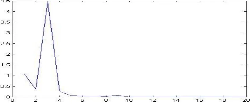
[image:2.595.100.529.277.466.2]

W(ω)=〖((m-1))/4〗^2 a〖sinc〗^2 (M-1)/2(ω) Here in this figure we see the generation of triangular window from the convolution of two rectangular windows.

Fig 1: generation of triangular window

[image:3.595.105.497.86.333.2]

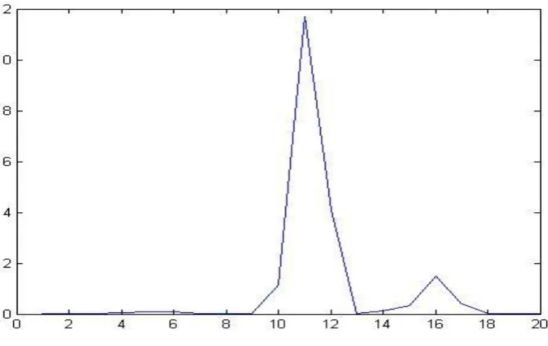
Fig: 2 Here is the figure where the energy of the signal within each

[image:3.595.91.484.417.654.2]

Finally after transforming the voice in to MEL FREQUENCY CEPSRTUM COEFFICIENT we get the

The complete coding involving this process is given below: clc;

fs = 10000; % Sampling Frequency

t = hamming(4000); % Hamming window to smooth the speech signal

w = [t ; zeros(6000,1)]; f = (1:10000);

mel(f) = 2595 * log(1 + f / 700); % Linear to Mel frequency scale conversion

tri = triang(100);

win1 = [tri ; zeros(9900,1)]; % Defining overlapping triangular windows for

win2 = [zeros(50,1) ; tri ; zeros(9850,1)]; % frequency domain analysis

win3 = [zeros(100,1) ; tri ; zeros(9800,1)]; win4 = [zeros(150,1) ; tri ; zeros(9750,1)]; win5 = [zeros(200,1) ; tri ; zeros(9700,1)]; win6 = [zeros(250,1) ; tri ; zeros(9650,1)]; win7 = [zeros(300,1) ; tri ; zeros(9600,1)]; win8 = [zeros(350,1) ; tri ; zeros(9550,1)]; win9 = [zeros(400,1) ; tri ; zeros(9500,1)]; win10 = [zeros(450,1) ; tri ; zeros(9450,1)]; win11 = [zeros(500,1) ; tri ; zeros(9400,1)]; win12 = [zeros(550,1) ; tri ; zeros(9350,1)]; win13 = [zeros(600,1) ; tri ; zeros(9300,1)]; win14 = [zeros(650,1) ; tri ; zeros(9250,1)]; win15 = [zeros(700,1) ; tri ; zeros(9200,1)]; win16 = [zeros(750,1) ; tri ; zeros(9150,1)]; win17 = [zeros(800,1) ; tri ; zeros(9100,1)]; win18 = [zeros(850,1) ; tri ; zeros(9050,1)]; win19 = [zeros(900,1) ; tri ; zeros(9000,1)]; win20 = [zeros(950,1) ; tri ; zeros(8950,1)];

x = wavrecord(1 * fs, fs, 'double'); % Record and store the uttered speech

%plot(x); wavplay(x);

x1 = x.* w;

mx = fft(x1); % Transform to frequency domain nx = abs(mx(floor(mel(f)))); % Mel warping nx = nx./ max(nx);

nx1 = nx.* win1; nx2 = nx.* win2; nx3 = nx.* win3; nx4 = nx.* win4; nx5 = nx.* win5; nx6 = nx.* win6; nx7 = nx.* win7; nx8 = nx.* win8; nx9 = nx.* win9; nx10 = nx.* win10; nx11 = nx.* win11; nx12 = nx.* win12; nx13 = nx.* win13; nx14 = nx.* win14; nx15 = nx.* win15; nx16 = nx.* win16; nx17 = nx.* win17; nx18 = nx.* win18; nx19 = nx.* win19; nx20 = nx.* win20;

sx1 = sum(nx1.^ 2); % Determine the energy of the signal within each window

sx2 = sum(nx2.^ 2); % by summing square of the magnitude of the spectrum

sx17 = sum(nx17.^ 2); sx18 = sum(nx18.^ 2); sx19 = sum(nx19.^ 2); sx20 = sum(nx20.^ 2);

sx = [sx1, sx2, sx3, sx4, sx5, sx6, sx7, sx8, sx9, sx10, sx11, sx12, sx13, sx14, sx15, sx16, sx17, sx18, sx19, sx20]; dx = dct(sx); % Determine DCT of Log of the spectrum energies

%plot(dx);

fid = fopen('sample.dat', 'w');

fwrite(fid, dx, 'real*8'); % Store this feature vector as a .dat file

fclose(fid);

5.

MATCHING OF VOICE

The matching or the testing part can be done by several methods. 1. Dynamic time wrapping 2. Vector Quantization 3. Hidden Markov Model.

5.1 Dynamic Time Wrapping:

In this process two signals are compared in time domain.

Dynamic time warping (DTW) finds the optimal alignment between two time series if one time series may be “warped” non-linearly by stretching or shrinking it along its time axis. This warping between two time series can then be used to find corresponding regions between the two time series or to determine the similarity between the two time series.[4]

First the signal to be tested is compared with the signal stored in the system. This is done by wrapping the time of the signal of the later and bringing two signals in same time frame and then it is needed to compare them. The comparison is done by measuring the distance of points of two signals and summing them [3].

A dynamic programming approach is used to find this minimum-distance warp path. Instead of attempting to find the path at once we need to calculate the distance between two

points and add them to find the minimum distance path. A two-dimensional m×n distance matrix D, is constructed where the value at D(i, j) is the minimum distance warp path.[4] let, we have two wrapped signals[3]

X: (x1,x2,….,xm)

Y: (y1,y2,…., yn)

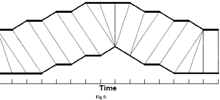
D(i, j)= (xi-y2)2 In FIG-5 we see two signals are compared and the optimal wrapped path is determined by the lines between two points and the path is the sum of the distance.

Optimizations to the DTW algorithm can be done by observing the minimum path from the list of paths. These are outlined in summarized as:[5]

5.1.1 Monotonic condition

:

the path will not turn back on itself, both I and j indexes either stay the same or increase, they never decrease.

5.1.2 Continuity condition

: The path advances one step at a time. Both i and j can only increase by 1 on each step along the path.

5.1.3 Boundary condition

: the path starts at the bottom left and ends at the top right.

5.1.4 Adjustment window condition

: a good path is unlikely to wander very far from the diagonal. The distance that the path is allowed to wander is the window length r.

[image:5.595.79.518.479.679.2]

5.1.5 Slope constraint condition

: The path should not be too steep or too shallow. This prevents very short sequences matching very long ones. The condition is expressed as a ratio n/m where m is the number of steps in the x direction and m is the number in the y direction. After m steps in x you must make a step in y and vice versa.

5.2 Vector Quantization:

This quite easy to implement and gives higher accuracy than the process described before. In this method we divide a large set of data into few small groups.

The flowchart of algorithm used to implement this vector quantization is LBG algorithm.

The flowchart is as follows:

no

Actually In vector quantization, the vector x is mapped onto another real-valued, discrete-amplitude, N dimensional vector

y. It is said that x is quantized as y, and y is the quantized value of x. We write Y = f(x) where f(.) is the quantization operator. y is also called the reconstruction vector or the

output vector corresponding to x.[6]

The block first received is divided further by following some certain rules. Then the distortion measure d(x, y) can be defined between x and y. d(x, y) is also known as a dissimilarity measure or distance measure.[6]

Then the average distortion is calculated by making arithmetic mean of set of data of distortions. That is the average distortion is simple mean point of dissimilarity. Then the recognition is done by comparing the mean distortion with

FIG-7

The density matching property of vector quantization is gives low error rate for identifying the density of large and high-dimensioned data. In the figure, only two speakers and two dimensions of the acoustic space are shown.[7]

5.3 Hidden Markov Modeling:

The last but most powerful tool used is Hidden Markov Modeling. HMM is such a method where symbols in sequence are detected. Working principle of HMM algorithm is based on probabilistic transition from one state to another in a finite state machine model.[11] HMM have a set of elements with hidden states and another set of elements from observations. Let the set of observations are given by O= {O1, O2, O3… OT} and P1 is the probability matrix of transitions, P2 is the probability matrix of output and P3 be initial probability matrix. The HMM is defined by a triplet consisting of three probability matrices (P1, P2, P3). [10]

One should follow some procedures to use HMMs in speech recognition:

O3… OT} and a HMM = (P1, P2, P3)

P3) to maximize P (O | HMM). [8]

6.

CODING FOR RECOGNITION:

clc;

fs = 10000; % Sampling Frequency

t = hamming(4000); % Hamming window to smooth the speech signal

w = [t ; zeros(6000,1)];

f = (1:10000);

mel(f) = 2595 * log(1 + f / 700); % Linear to Mel frequency scale conversion

tri = triang(100);

win1 = [tri ; zeros(9900,1)]; % Defining overlapping triangular windows for

win2 = [zeros(50,1) ; tri ; zeros(9850,1)]; % frequency domain analysis

Find centroid

Split each centroid

M=2m

Cluster vectors

Find centroids

Compute D=(distortion)

(D’-D)/D< ɛ

m<M

D’=D

s

t

o

p

Yes Yes

no

A A B B

A AA BBB

a b

AAA BBB

a b

AAA BBB

win7 = [zeros(300,1) ; tri ; zeros(9600,1)];

win8 = [zeros(350,1) ; tri ; zeros(9550,1)];

win9 = [zeros(400,1) ; tri ; zeros(9500,1)];

win10 = [zeros(450,1) ; tri ; zeros(9450,1)];

win11 = [zeros(500,1) ; tri ; zeros(9400,1)];

win12 = [zeros(550,1) ; tri ; zeros(9350,1)];

win13 = [zeros(600,1) ; tri ; zeros(9300,1)];

win14 = [zeros(650,1) ; tri ; zeros(9250,1)];

win15 = [zeros(700,1) ; tri ; zeros(9200,1)];

win16 = [zeros(750,1) ; tri ; zeros(9150,1)];

win17 = [zeros(800,1) ; tri ; zeros(9100,1)];

win18 = [zeros(850,1) ; tri ; zeros(9050,1)];

win19 = [zeros(900,1) ; tri ; zeros(9000,1)];

win20 = [zeros(950,1) ; tri ; zeros(8950,1)];

y = wavrecord(1 * fs, fs, 'double'); %Store the uttered password for authentication

i = 1;

while abs(y(i)) < 0.05 % Silence Detection

i = i + 1;

end

y(1 : i) = [];

y(6000 : 10000) = 0;

y1 = y.* w;

my = fft(y1); % Transform to frequency domain

ny = abs(my(floor(mel(f)))); % Mel warping

ny = ny./ max(ny);

ny1 = ny.* win1;

ny2 = ny.* win2;

ny3 = ny.* win3;

ny4 = ny.* win4;

ny5 = ny.* win5;

ny6 = ny.* win6;

ny7 = ny.* win7;

ny8 = ny.* win8;

ny9 = ny.* win9;

ny10 = ny.* win10;

ny11 = ny.* win11;

ny12 = ny.* win12;

ny18 = ny.* win18;

ny19 = ny.* win19;

ny20 = ny.* win20;

sy1 = sum(ny1.^ 2);

sy2 = sum(ny2.^ 2);

sy3 = sum(ny3.^ 2);

sy4 = sum(ny4.^ 2);

sy5 = sum(ny5.^ 2);

sy6 = sum(ny6.^ 2);

sy7 = sum(ny7.^ 2);

sy8 = sum(ny8.^ 2);

sy9 = sum(ny9.^ 2);

sy10 = sum(ny10.^ 2); % Determine the energy of the signal within each window

sy11 = sum(ny11.^ 2); % by summing square of the magnitude of the spectrum

sy12 = sum(ny12.^ 2);

sy13 = sum(ny13.^ 2);

sy14 = sum(ny14.^ 2);

sy15 = sum(ny15.^ 2);

sy16 = sum(ny16.^ 2);

sy17 = sum(ny17.^ 2);

sy18 = sum(ny18.^ 2);

sy19 = sum(ny19.^ 2);

sy20 = sum(ny20.^ 2);

sy = [sy1, sy2, sy3, sy4, sy5, sy6, sy7, sy8, sy9, sy10, sy11, sy12, sy13, sy14, sy15, sy16, sy17, sy18, sy19, sy20];

sy = log(sy);

dy = dct(sy); % Determine DCT of Log of the spectrum energies

fid = fopen('sample.dat','r');

dx = fread(fid, 20, 'real*8'); % Obtain the feature vector for the password

fclose(fid); % evaluated in the training phase

dx = dx.';

MSE=(sum((dx - dy).^ 2)) / 20; % Determine the Mean squared error

if MSE<1.5

fprintf('\n\nYou are the same user\n\n');

% end

%end

%fclose(s);

%delete(s);

%Grant=wavread('Grant.wav'); % “Access Granted” is output if within threshold

%wavplay(Grant);

else

fprintf('\n\nYou are not a same user\n\n');

%s=serial('COM8');

%fopen(s);

%fprintf(s,'b');

%for i=1:1:500

% for j=1:1:500

% end

%end

%fclose(s);

%delete(s);

%Deny=wavread('Deny.wav'); % “Access Denied” is output in case of a failure

%wavplay(Deny);

end

7.

CONCLUSION

The accuracy level achieved in this format is almost above 80% in both male and female. Later the integration of LPCC with MFCC can be investigated for this purpose. If the efficiency of this recognition could be increased over 90% this can be used for different biometric tests like retina scan and finger print scan. This process can be used to grant access in different zones like ATM machine, Automation of the system and many other fields.

Now it is seen that a very little use of voice as a means of recognizing a person. But at first our tendency is to recognize a person by his/her voice. So artificial intelligence will be boosted by a large extent if we can increase the efficiency of recognizing the voice by machinery method.

8.

REFERENCES

[1] Ashish jain,hohn harris,speaker identification using mfcc andhmm based techniques,university of florida,april 25,2004

[2] “Mel frequency cepstral coefficient for music modeling” beth logan cambridge research laboratory

[3] Voice recognition algorithms using mel frequency cepstral coefficient (mfcc) and dynamic time warping (dtw) techniques lindasalwa muda, mumtaj begam and i. Elamvazuthi.

Journal of computing, volume 2, issue 3, march 2010, issn 2151-9617

[4] Fast dtw: toward accurate dynamic time warping in linear time and space stan salvador and philip chan dept. Of computer sciences florida institute of technology melbourne, fl 32901

[5] http://web.science.mq.edu.au/~cassidy/comp449/html/ch 11s02. Html, downloaded on 3rd march 2010.

[6] Vector quantization in speech coding john makhoul, fellow ieee, salim roucos, member ieee and herbet gish member ieee

[7] “Performance improvement of speaker recognition system” anand vardhan bhalla, master of technology, Gyan ganga college of technology jabalpur (m.p.) India. E-mail: [email protected] Shailesh khaparkar (asst. Prof.) Head of department, Electrical and electronics engg. Gyan ganga college of technology jabalpur (m.p.) India.

[8] “Speech recognition with hidden markov model: a review”-- bhupinder singh, neha kapur, puneet kaur Dept. Of computer sc. & engg., igce abhipur, mohali (pb.), india

[9] “Artificial neural network for speech recognition”--- austin marshall. March3, 2005

[10] “A novel voice recognition model based on hmm and fuzzy ppm” -- zhang, j. G&ps (r&d), motorola china, chengdu, china wang, b.