Efficiency of Selecting Important Variable for Longitudinal Data

Published Online January 2014 in SciRes (http://www.scirp.org/journal/psych) http://dx.doi.org/10.4236/psych.2014.51002

Efficiency of Selecting Important Variable for Longitudinal Data

Jongmin Ra, Ki-Jong Rhee

Department of Education, Kookmin University, Seoul, South Korea Email: [email protected]

Received October 12th_{, 2013; revised November 13}th_{, 2013; accepted December 9}th_{, 2013}

Copyright © 2014 Jongmin Ra,Ki-Jong Rhee. This is an open access article distributed under the Creative Commons Attribution License, which permits unrestricted use, distribution, and reproduction in any medium, provided the original work is properly cited. In accordance of the Creative Commons Attribution License all Copyrights © 2014 are reserved for SCIRP and the owner of the intellectual property Jongmin Ra,Ki-Jong Rhee. All Copyright © 2014 are guarded by law and by SCIRP as a guardian.

Variable selection with a large number of predictors is a very challenging and important problem in edu-cational and social domains. However, relatively little attention has been paid to issues of variable selec-tion in longitudinal data with applicaselec-tion to educaselec-tion. Using this longitudinal educaselec-tional data (Test of English for International Communication, TOEIC), this study compares multiple regression, backward elimination, group least selection absolute shrinkage and selection operator (LASSO), and linear mixed models in terms of their performance in variable selection. The results from the study show that four dif-ferent statistical methods contain difdif-ferent sets of predictors in their models. The linear mixed model (LMM) provides the smallest number of predictors (4 predictors among a total of 19 predictors). In addi-tion, LMM is the only appropriate method for the repeated measurement and is the best method with re-spect to the principal of parsimony. This study also provides interpretation of the selected model by LMM in the conclusion using marginal 2

R .

Keywords: Group LASSO; Linear Mixed Model; Longitudinal Data; Marginal 2

R ; Variable Selection

Introduction

The characteristic of a longitudinal study is that individuals are measured repeatedly through different time points and re-quire special statistical methods because the set of observations on the same individual tends to be inter-correlated and can be explained by both fixed and random effects.

As longitudinal data are common in educational settings, the linear mixed model (LMM) has emerged as an effective ap-proach since it can model within and between subject hetero-geneity (Vonesh, Chinchilli, & Pu, 1996). The LMM also at-tempts to account for within-subject dependency in the multiple measurements by including one or more subject-specific vari-ables in a regression model (Laird & Ware, 1982; Giks, Wang, Yvonnet, & Coursaget, 1993).

Despite the development of statistical models, model selec-tion criteria for the LMM have received little attenselec-tion (Orelien & Edwards, 2008; Vonesh et al., 1996). However, several stud-ies (Vonesh & Chinchilli, 1997; Vonesh et al., 1996; Zheng, 2000) recently suggest model fit indices which are useful for mixed effect models. More specifically, studies (Vonesh & Chinchilli, 1997; Vonesh et al., 1996) show that marginal 2

R

is preferred when only fixed-effect components are involved in the predicted values, but conditional 2

R is preferred for ran-dom effects (Vonesh et al., 1996).

It is not uncommon to collect a large number of predictors to model an individual’s reading achievement more accurately in educational and psychological fields. Thus, it is fundamental to select meaningful variables in multivariate statistical models (Zhang, Wahba, Lin, Voelker, Ferris, Klein, & Klein, 2004) to increase prediction accuracy and to provide better

understand-ing of concepts.

It is, however, challenging to select important variables when a response variable is measured repeatedly over a certain period of time because it is known that the selection process of statis-tically significant variables is hindered by the correlation among the repeated measurements. Furthermore, classical vari- able selection methods, such as the forward selection and the backward elimination methods are time-consuming, unstable, and sometimes unreliable for making inferences. Although there is a great deal of extent research examining issues of vari- able selection in linear regression, little research has been done investigating how differently and similarly different statistical methods perform within a longitudinal data. This study aims to investigate how similarly and differently various statistical methods perform in the presence of the repeated measurements in the data.

Hence, this study compares four different statistical methods, multiple regression, backward elimination, group least selection absolute shrinkage and selection operator (LASSO), and the LMM, using a test of English as International Communication (TOEIC) data as individuals’ reading achievement. For the LMM, marginal 2

R for remaining variables in the model is used to provide a better understanding of the impacts of se-lected predictors in the longitudinal data.

Multiple Linear Regression

West, & Aiken, 2003). For instance, if a multiple regression method is used for predicting and explaining an individual’s English achievement, many variables such as gender, age, and socio-economic status (SES) might all contribute toward indi-vidual’s English achievement.

The multiple regression method for predicting English achieve-ment, Y, with the observed data

(

X_{1 ,i},X_pi

)

,i=1,, ,n is as follows Yi=β0+β1X1i+β2X2i+ + βpXpi+εi. This equation shows the relationship between p predictors and a response variable Y, all of which are measured simultaneously on the subject. This method is called linear because the effects of the various predictors are treated as additive.

In addition, much efforts has been put to estimate the per-formance of different methods and choose the best one by using fit indices such as AIC (Akaike, 1973), BIC (Schwarz, 1978), Mellow’s Cp (Mallows, 1973), and adjusted

2

R . AIC and BIC are based on the penalized maximum likelihood estimates. AIC is defined as −2log(L) + 2p, where log(L) is the loglikeli-hood function of the parameters in the model evaluated at the maximum likelihood estimator while the second term is a pen-alty term for additional parameters in the model. Therefore, as the number of independent variables included in the model increases, the first term decreases while the penalty term in-creases. Conversely, as variables are dropped from the model, the lack of fit term increases while the penalty term decreases. BIC is defined as −2log

( )

L + ×p log

( )

n . The penalty term for BIC is similar to AIC but uses a multiplier of log(n) instead of a constant 2 by incorporating the sample size. In general, AIC tends to choose overly complex models when sample size is large and BIC tends to choose overly simple model when ple size is small and also choose the correct model when sam-ple size approaches infinity.

Mallow’s Cp is also commonly used to investigate how well a model fits data and can be defined as C_p=(SSE_p σ2)+2p+n



. In this equation, ˆσ represents the estimate of _{σ and} 2

p

SSE is defined as

(

)

2

1 1

ˆ

n p

i ii

i= Y − i=X β

∑

∑

, where ˆβ is the estimator of β. Mallow’s Cp is calculated for all possible subset models. The model with the smallest value of Cp is deemed to be the best linear model. As the number of independent variables (p) increases, an increased penalty term 2p is offset with a decreased SSE.

Another commonly used fit index for model selection is 2

R

or adjusted 2

R . Both 2

R and adjusted 2

R represent the percentage of the variability of the response variable that is explained by the variation of predictors. 2

R is a function of the total sum of square (SST) and SSE, and the formula is given by

(

1−SSE SST

)

.

Adjusted 2

R takes into account the degrees of freedom used up by adding more predictors. Even though adjusted 2

R

attempts to yield a more robust value to estimate 2

R , there is little difference between adjusted 2

R and 2

R when a large number of predictors are included in a model.

When the number of observations is very large compared to the number of predictors in a model, the value of 2

R and ad-justed 2

R will be much closer because the ratio of

(

n 1−

) (

n− −p 1

)

will approach 1. Despite the practical ad-vantages of using a multiple regression method, it is difficult to build multiple regression models for repeatedly measured re-sponses. The multiple regression method is not appropriate for correlated response variables as in longitudinal data without accounting for correlation within response variables.

Backward Elimination Approach

Besides the multiple regression approach, backward elimina-tion is common and important practice to select relevant vari-ables among a large number of predictors. A subset selection method is one of the most widely used variable selection ap-proaches in which one predictor at a time is added or deleted based on the F statistic iteratively (Bernstein, 1989). Subset selection methods, in general, provide an effective means to screen a large number of variables (Hosmer & Lmeshow, 2000). Since there is a possibility of emerging a suppressor effect in the forward inclusion method (Agresti & Finlay, 1986), the backward elimination method is usually preferred method of exploratory analysis (Agresti, 2002; Hosmer & Lemeshow, 2000; Menard, 1995) and follows three steps.

First, obtains a regression equation which includes allp pre-dictors. Second, conducts a partial F-test for each of the pre-dictors which indicates the significance of the corresponding predictor as if it is the last variable entered into the equation. Finally, selects the lowest partial F value and compares it with a threshold partial, Fα, the value set equal to some predeter-mined level of significance,

α

If the smallest partial F is less than Fα, then deletes that variable and repeats the process for

p − 1 predictors. This sequence continues until the smallest partial Fα at any given step is greater than Fα. The variables that are remained in the model are considered as significant predictors. In general, the backward elimination method is computationally attractive and can be conducted with an esti-mation accuracy criterion or through hypothesis testing.

The backward elimination method, however, is far from per-fection. This method often leads to locally optimal solutions rather than globally optimal solution. Also, the backward elimination method yields confidence intervals for effects and predicted value that are far too narrow (Altman & Andersen, 1989). The degree of correlation among the predictors affects the frequency with which authentic predictor find their way into the final model in terms of frequency of obtaining authentic and noise predictors (Derksen & Keselman, 1992). More specifi-cally, the number of candidate predictors affects the number of noise predictors that gains entry to the model. Furthermore, it is well known that the backward elimination method will not necessarily produce the best model if there are redundant vari-ables (Derksen & Keselman, 1992). It also yields 2

R values that are badly biased upward and have severe problems in the presence of collinearity. Since the backward elimination me- thod gives biased regression coefficient estimates, they need to be shrunk because the regression coefficients for remaining variables are too large. Besides well-known inherent technical problems, it is time consuming when a large number of predic-tors are included in the model and cumbersome to choose ap-propriate variables manually when categorical variables are included in the model as a dummy variable.

The Group LASSO

(LASSO) suggested by Tibshirani (1996) is one of well-known penalized regression approaches (Bondell & Reich, 2008; Meier, van de Geer, & Bhlmann, 2008; Tibshirani, 1996). The LASSO method minimizes the residual sum of squares subject to the sum of the absolute value of the coefficients being less than a constant (Tibshirani, 1996). It is also well known that all the variables in LASSO type methods such as the standardized LASSO and group LASSO (Yuan & Lin, 2006) need to be standardized before performing analysis.

The LASSO method is defined as follows

( )

(

)

2

0

1 0 1

ˆ min

arg n p p

LASSO β i Y i Xii i

β λ =

∑

₌ −

∑

₌ β +λ

∑

₌ β In this equation, β=

(

β β₀, ₁,β_p

)

and λ is a penalty or tuning parameter. The parameter𝛌𝛌controls the amount of shrinkage that is applied to the estimates. The solution paths of LASSO are piecewise linear, and thus can be computed very efficiently. The variables selected by the LASSO method are included in the model with shrunken coefficients. The salient feature of the LASSO method is that it sets some coefficients to be 0 and shrinks others. Furthermore, the LASSO method has two ad-vantages compared to the traditional estimation method. One is that it estimates parameters and select variables simultaneously (Tibshirani, 1996; Fan & Li, 2001). The other is that the solu-tion path of the LASSO method moves in a predictable manner sine it has good computational properties (Efron, Hastie, Johnstone, & Tibshirani, 2004). Thus, the LASSO method can be used for high-dimensional data as long as the number of predictors, is smaller than or equal ton, p≤n.

The LASSO method, however, has some drawbacks (Yuan & Lin, 2006). If the number of predictors (p) is larger than the number of observations (n), the LASSO method at most select variables due to the nature of the convex optimization problem. Also, the LASSO method tends to make selection based on the strength of individual derived input variables rather than the strength of groups of input variables, often resulting in select-ing more variables than necessary. Another drawback of usselect-ing the LASSO method is that the solution depends on how the variables are orthonormalized. That is, if any variable X_i is reparameterized through a different set of orthonormal contrasts, there is a possibility of getting different set of variables in the solution. This is undesirable since solutions to a variable selec-tion and estimaselec-tion problem should not depend on how the variables are represented. In addition, the LASSO solutions bring another problem when categorical variables enter into the model. The LASSO method treats categorical variables as an individual variables rather than a group (Meier et al., 2008). A major stumbling block of the LASSO method is that if there are groups of highly correlated variables, it tends to arbitrarily se-lect only one from each group. This makes models difficult to interpret because predictors that are strongly associated with the outcome are not included in the predictive model.

To remedy the shortcomings of the LASSO method, Yuan and Lin (2006) suggested the group LASSO in which an entire group of predictors may drop out of the model depending on. The group LASSO is defined as follows

( )

2

1 1 1

1 1

min

arg L p

LASSO Y l Xll i P

β λ = _ −

∑

₌ +λ

∑

₌ β _ In this equation, X_l represents the predictors corresponding to the

lth group, with corresponding coefficient sub-vector, and β_l. l

P takes into account for the different group sizes. If

(

1,

)

T k

x= x x , then, 2 2

1 1

k i i

x =

∑

₌x . The group LASSO acts

like the LASSO at the group level; depending λ , an entire group of predictors may drop out of the model. The group LASSO takes two steps. First, a solution path indexed by cer-tain tuning parameter is built. Then, the final model is selected on the solution path by cross validation or using a criterion such as the Mallow’s Cp.

This gives group LASSO tremendous computational advan-tages when compared with other methods. The group LASSO makes statistically insignificant variables become zero by in-corporating shrinkage as the standard LASSO does. Overall, the group LASSO method enjoys great computational advantages and excellent performance, and a number of nonzero coeffi-cients in the LASSO and the group LASSO methods are an unbiased estimated of the degree of freedom (Efron et al., 2004).

Even though the group LASSO is suggested for overcoming drawbacks for the standard LASSO, the group LASSO method still has some limitations. For example, the solution path of the group LASSO is not piecewise linear which precludes the ap-plication of efficient optimization methods (Efron et al., 2004). It is also known that the method tends to select a large number of groups than necessary, and thus includes some noisy vari-ables in the model (Meier et al., 2008). Furthermore, the group LASSO method is not directly applicable to longitudinal data and needs further study for being suitable for the repeated measurement. R code for the group LASSO is provided in

Appendix.

Linear Mixed Model

The linear mixed model (LMM) is another very useful ap-proach for longitudinal studies to describe relationship between a response variable and predictors. The LMM has been called differently in different fields. In economics, the term “random coefficient regression models” is common. In sociology, “mul-tilevel modeling” is common, alluding to the fact that regres-sion intercepts and slops at the individual level may be treated as random effects of a higher level. In statistics, the term “variance components models” is often used in addition to mixed effect models, alluding to the fact that one may decom-pose the variance into components attributable to within-groups versus between-groups effects. All these terms are closely re-lated, albeit emphasizing different aspects of the LMM. In the context of repeated measure, let Y_i is an ni×1 vector of observations from the ith subject. Then, the LMM (Laird & Ware, 1982) is as follows Y_i=X_iβ+Z b_{i i}+ε_i.

In this model,

(

1 , ,

)

T t

i i pi

X = X _X , where X_i is ann_i×p

fixed effect design matrix whereas Z_i are known n_i×q

constant design matrices. β=

(

β₁,βp

)

T is an p-dimensional vector and unknown coefficients of the fixed effects. Here, b_i

Method

Participants and Variables

This study takes place in a public university in Republic of Korea, between the years 2009 and 2010, over two semesters. Participating students (n = 281) enrolled in TOEIC classes for four hours a week. Except students’ TOEIC scores, The TOEIC dataset records 20 predictors. Among 20 predictors, 13 are continuous: age, father’s education level (FEL), mother’s edu-cation level (MEL), SES, English study time (EST), reading time, level of reading competence (LRC), materials written in English (ME), level of computer skill (LC), length of private tutoring (LPT), three mean-centered cognitive assessment scores (STAS: State and trait anxiety scale, FLCAS: Foreign language classroom anxiety scale, FRAS: Foreign language reading anxiety scale); and 7 are categorical: major, gender, ex- perience of private tutoring (EPT), experience of having foreign instructors (EFI), living areas, length of staying at abroad (LSA), experience of staying English speaking countries (ESE). The wave 2, 3, and 4 data are collected every three months after collecting wave 1 data.

Procedures

All the analysis are performed with R (R Development Core Team, 2013) due to the unavailability of the group LASSO approach in standardized statistical packages such as SPSS. Once statistically significant predictors in the model are ob-tained, goodness-of-fit for the LMM can be considered. Among different types of 𝑅𝑅2such as unweighted concordance correla-tion coefficient (CCC: Venesh et al., 1996), and proporcorrela-tional reduction in penalized quasi-likelihood (Zheng, 2000), the mar-ginal 2

R (Vonesh & Chinchilli, 1997) is easy to compute and interpret in that it is a straightforward extension of the tradi-tional 2

R (Orelien & Edwards, 2008). The marginal 2

R in this analysis for selecting relevant variables is defined as follows

(

) (

)

(

1

) (

)

2

1

ˆ ˆ

1

T n

i i i i

m n T

i pi i pi i

Y Y Y Y R

Y Y Y Y

=

=

− −

= −

− −

∑

∑

.

Given the equation shown above,𝑌𝑌_𝑖𝑖,nof observations, is a observed response variable and ˆY_i is a predicted response variables.Y_i is the grand mean and is an vector of 1’s. This equation implies Yˆ=Xβˆ and considers only fixed effects. In addition, marginal𝑅𝑅2modeling the average subject (Yˆ=Xβˆ) leads to the terms average model (Vonesh & Chinchilli, 1997) where 2

m

R is the proportionate reduction in residual variation explained by the modeled response of the average subject. Thus, when important predictors in the model are not included, the values of marginal 2

R decrease sharply. If the random effects are excluded in the computation of the predicted values that lead to the residuals, the marginal 2

R is able to select the most parsimonious model.

Results

For descriptive analysis, frequencies and percentages of all variables are calculated. Regarding categorical variables, there are 9 different majors having similar number of students who are participated in this study except two majors (Child Educa-tion and OccupaEduca-tional Therapy major) which consist of less than 10% of total sample sizes, respectively. Also, there are the

smallest number of students (n = 14) in Child Education major compared to other majors. Relatively a large number of stu-dents (n = 35) from the Chung-Nam areas are participated. In accordance with the experiences of having classes with for-eign-instructors, about 44.9% of students do not have any ex-perience. About 15.7% of them have experience studying abroad and 29.2% are male. Furthermore, almost 60% of stu-dents never have a private tutoring.

For continuous variables, the mean and standard deviation of continuous variables are calculated. In terms of outcomes across 4 wave points, reading scores of TOEIC are increased as time increases, 234.69, 274, 94, 264.75, and 284.03 respec-tively. However, scores of TOEIC are slightly dropped between wave 2 and wave 3. The average age of students is 20.11 years old. The average education level of fathers (3.42) is little higher than that of mothers (3.13). Furthermore, the significantly ferent TOEIC scores across four waves are shown among dif-ferent majors. Furthermore, Figure 1 shows that students in medical major has high initial TOEIC scores.

The existence of relationship between reading achievement and predictors across wave 1, wave 2, wave, 3 and wave 4 is analyzed using four separate multiple regression runs. Results show that there are four majors statistically significant majors (medical, nursing, e-business, tourism) across 4 wave points. Besides students’ major, four separate multiple regression models contains only one variable (LRC) across four wave points in common.

[image:4.595.311.539.530.712.2]

Results are also obtained from the four separated backward elimination procedures for the each wave, including nineteen predictors in the full model. Only five majors (medical, nursing, e-business, tourism, childcare majors) are statistically signifi-cant across four wave points. Besides individual’s major, there are seven significant predictors across four separate analyses; two variables (MEL and LRC) at the first, two variables (ME and LRC) for the second wave, one variable (LRC) at the third, and six variables (gender, FEL, EST, ME, LRC and STAI) at the fourth wave point. The interesting point is that four separate backward elimination procedures contain different sets of pre-dictors in the model. It might imply that the backward elimina-tion method is not suitable for dealing with the repeated meas-urement.

Figure 1.

Compared to the backward elimination method, the group LASSO contains more predictors in the model. In addition, four separate group LASSO procedures contain different types of predictors. Besides students’ major, total seventeen predictors are included across four separate models; fourteen variables (gender, age, area, FEL, MEL, EFI, EST, ME, LRC, LSA, LPT, LC, STAI, and FLRAS) are selected in the first wave, then ten variables (place, MEL, ME, LRC, LSA, LPT, and STAI) in the second wave, nine variables (gender, income, MEL, ME, LRC, LSA, EPT, LC, and STAI) in the third wave, and nine variables (age, area, FEL, EST, ME, LRC, LC, STAI, and FLRAS) in the fourth wave.

Compared to multiple regression and backward elimination method, the group LASSO includes more categorical variables, such as area, place, and length of staying abroad in the finalized model. However, the results show that four separate group LASSO methods also contain different sets of predictors in the model. This might suggest inappropriateness of using the group LASSO to the repeated measurement.

Results obtained from the LMM show that all the majors and four continuous explanatory variables (MEL, LST, ME, and LRC) are included in the finalized model. The results reveal that TOEIC achievement is positively related with MEL (p

< .05), LST (p < .01), and LRC (p < .01) but negatively related ME (p < .01). Interesting finding is that ME positively affects TOEIC achievement positively in univariate analysis but affects TOEIC achievement negatively when considered ME condi-tional on students’ major, LRC, LST, and MEL.

Once selecting statistically significant predictors in the model, changes of marginal 2

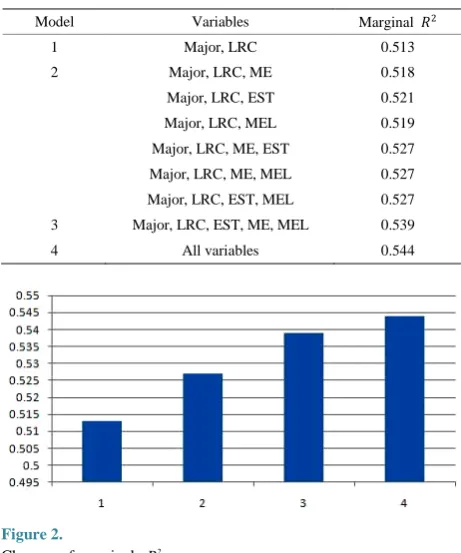
R across all possible combina-tions of predictors are calculated in Table 1. Table 1 shows that Model 1 only contains MAJOR and LRC in the model. Model 2 includes MAJOR and LRC with other three predictors (MS, LST and MEL). To identify which predictors mostly af-fect TOEIC achievement, marginal 2

R for all possible combi-nations within Models 2 are also considered.

However, there is less variations among all possible combi-nations in Model 2. Values of the marginal 2

R for all possible combinations of the selected predictors range from .518 to .527. Model 3 contains five predictors: students’ major, LRC, EST, ME, and MEL predictors selected from the LMM. Finally, Model 4 includes all twenty predictors in the model.

Valued of four different marginal 2

R s for Model 1, Model 2, Model 3 and Model 4 are .513, .527, .539, and .544, respec-tively. Figure 2 also describes the changes of marginal 2

R

across four different models.

As shown in Figure 2, there is less changes of marginal 2

R

(.005) between Model 4 including nineteen predictors and Model 3 including 5 predictors. However, compared to changes of marginal 2

R from Model 4 to Model 3, changes of mar-ginal 2

R from Model 3 to Model 2 is relatively large, .012. This result suggests that four continuous variables (LRC, ME, EST, and MEL) should be included in the model.

Conclusion and Discussion

This study examines the relation of TOEIC achievement and twenty predictors under four different statistical methods. Dif-ferent sets of predictors are selected in four difDif-ferent statistical methods. The results show that there is a strong evidence to support the existence of relation between TOEIC achievement and some predictors included in this study. Without considering

Table 1. Marginal 2

R for all possible combination.

Model Variables Marginal 𝑅𝑅2

1 Major, LRC 0.513

2 Major, LRC, ME 0.518

Major, LRC, EST 0.521

Major, LRC, MEL 0.519

Major, LRC, ME, EST 0.527

Major, LRC, ME, MEL 0.527

Major, LRC, EST, MEL 0.527

3 Major, LRC, EST, ME, MEL 0.539

[image:5.595.307.538.107.384.2]

4 All variables 0.544

Figure 2.

Changes of marginal 2

R .

other predictors, there are much variation in TOEIC reading achievement among nine different majors. As expected, stu-dents in medical program have high TOEIC scores compared to others in different programs. Thus, it is necessary to investigate predictors which affect growth of TOEIC scores while consid-ering group difference. Results from this study also show that LRC (levels of English ability) is a useful variable to explain and predict TOEIC achievement. Interestingly, LRC is signifi-cant across four different statistical methods. It makes sense since the levels of English ability affect TOEIC reading achievement positively across four waves. However, when negative relationship between EM and TOEIC achievement has emerged when considered ME predictor conditional on other predictors (major, LRC, EST, and MEL) in the model.

The LMM reveals that there is little variation in the values of marginal across all possible combinations of predictors in-cluded in the final model. Among four different statistical methods, the LMM model seems to be most effective and use-ful to build a parsimonious model with important and mean-ingful predictors because it takes into account the repeated measurements, which is flexible, and powerful to analyze bal-anced and unbalbal-anced grouped data. However, these results must be regarded as very tentative and inconclusive because this is a search for plausible predictors, not a convincing test of any theory. Further development based on these results would require replication with other data and explanation of why these variables appear as predictors of continuity of achievement.

among four statistical models is not pursued since the objective of this research is to test hypotheses based on theories.

Concerning the LASSO method, the group LASSO method enjoys great computational advantages and excellent perform-ance, and a number of nonzero coefficient in the LASSO and the group LASSO method are an unbiased estimate of the de-gree of freedom (Efron et al., 2004). However, it is necessary to consider the LASSO method in the hierarchical structure for further studies since experiment and survey designs should be included in the model. Then, the LASSO method in the LM model framework is useful to explain random effects. Despite the limitations listed above, this study would contribute to the field of education as a better way of explaining of relationship between personal predictors and English achievement.

REFERENCES

Agresti, A. (2002). Categorical data analysis (2nd ed.). Boboken, NJ: John Wiley & Sons.

Agresti, A., & Finlay, B. (1986). Statistical method for the social sci-ences (2nd, ed.). San Francisco, CA: Dellen.

Akaike, H. (1973). Information theory and an extension of the maxi-mum likelihood principle. In B. N. Petrov, & F. Csaki (Eds.), Second international symposium on information theory (pp. 267-281). Bu-dapest: AcademiaiKiado.

Altman, D. G., & Andersen, P. K. (1989). Bootstrap investigation of the stability of a Coxregression model. Statistics in Medicine, 8, 771-783. Bernstein, I. H. (1989). Applied multivariate analysis. New York:

Springer-Verlag.

Bondell, H. D., & Reich, B. J. (2008). Simultaneous regression shrink-age, variable selectionand clustering of predictors with OSCAR. Bio- metrics, 64, 115-123.

Cohen, J., Cohen, P., West, S. G., & Aiken, L. S. (2003). Applied mul-tipleregression/correlation analysis for the behavioral sciences (3rd ed.). Mahwah, NJ: Lawrence Erlbaum.

Derksen, S., & Keselman, H. J. (1992). Backward, forward and step-wise automated subset selection algorithms. British Journal of Ma- thematical and Statistical Psychology, 45, 265-282.

Efron, B., Hastie, T., Johnstone, I., & Tibshirani, R. (2004). Least angle regression. The Annals of Statistics, 32, 407-489.

Fan, J., & Li, R. (2001). Variable selection vianonconcave penalized likelihood and its oracle properties. Journal of the American Statis-tical Association, 96, 1348-1360.

Foster, D. P., & George, E. I. (1994). The risk inflation criterion for

multiple regression. The Annals of Statistics, 22, 1947-1975. George, E. I., & McCulloch, R. E. (1993). Variable selection via Gibbs

sampling. Journal of the American Statistical Association, 88, 881- 889.

Gilks, W. R., Wang, C. C, Yvonnet, B., & Coursaget, P. (1993). Ran- dom effects models for longitudinal data using Gibbs sampling. Bio- metrics, 49, 441-453.

Hosmer, D. W., & Lemeshow, S. (2000). Applied logistic regression. New York: John Wiley& Sons.

Laird, N., & Ware, J. H. (1982). Random effect models for longitudinal data. Biometrics, 38, 963-974.

Mallows, C. L. (1973). Some comments on Cp. Technometrics, 15, 611-675.

Meier, L., van de Geer, S., & Buhlmann, P. (2008). The group lasso for logistic regression. Journal of Royal Statistical Society, B, 70, 53-71. Menard, S. (1995). Applied logistic regression analysis (Sage university

paper series on quantitative application in the social sciences, series no. 106) (2nd ed.). ThousandOaks, CA: Sage.

O’Hara, R. B., & Sillanpaää, M. J. (2009). A review of Bayesian vari-able selection methods: what, how and which. Bayesian Analysis, 4, 85-118.

Orelien.,& Edwards, L. J. (2008). Fixed effect variable selection in linear mixed models using statistics. Computational Statistics & Data Analysis, 52, 1896-1907.

R Development Core Team. (2013). R: A language environment for statistical computing. Vienna, Austria: The R foundation for statisti-cal computing. http://www.R-project.org/

Schwarz, G. (1978). Estimating the dimension of a model. The Annals of Statistics, 6, 461-464.

Tibshirani, R. (1996). Regression shrinkage and selection via the lasso. Journal of Royal Statistical Society, B, 58, 267-288.

Vonesh, E. F., & Chinchilli, V. M. (1997). Linear and Nonlinear mod-els for the analysis of repeated measurement. New York: Marcel Dekker.

Vonesh, E. F., Chinchilli, V. M., & Pu, K. W. (1996).Goodness-of-fit in generalized nonlinear mixed-effects model. Biometrics, 52, 572-587. Yuan, M., & Lin, Y. (2006).The composite absolute penalties family for grouped and hierarchical variable selection. Journal of the Royal Statistical Society, B, 68, 49-67.

Zhang, H. H. Wahba, G., Lin, Y., Voelker, M., Ferris, M., Klein, R., & Klein, B. (2004). Variable selection and model building via like li-hood basis pursuit. Journal of the American Statistical Association, 99, 659-672.

Zheng, B. Y. (2000). Summarizing the goodness of fit of generalized linear models for longitudinal data. Statistics in Medicine, 19, 1265- 1275.

Appendix

Group LASSO (R code)

toeic.tr < -as.data.frame(toeic.group[ind[1:225],]) #GROUP LASSO

Cols < -ncol(toeic.tr)-1 index.lasso < -c(rep(0,cols)) numgr < -length(gr) stg < −1

ltg < -gr[1] for (i in 1:numgr) { index.lasso[(stg:ltg)] < -1 if (I < numgr) {

stg < -stg + gr[i]

ltg < -ltg + gr[I + 1] }

}

Lamda < -c(2000, 1500, 1000, 500, 100, 10, 1, 0.1, 0.01) fold < −10

lamda.lasso < -cvlasso Reg (y~., toeic.tr, fold, cvind, index. lasso, lam)

ini.lasso < -grplasso (x = as.matrix(toeic.tr[,-30]),

y = as.matrix(toeic.tr[,30]), index = index.lasso, lamda = lam. lasso, model = LinReg(), penscale = sqrt)

lasso.pred < -as.matrix (as.matrix (toeic.te [,−30]))% * % ini. Lasso $ coefficients