Delaware Method Improvement for the Shell and Tubes Heat Exchanger Design

http://dx.doi.org/10.4236/eng.2014.64023

Delaware Method Improvement for the Shell

and Tubes Heat Exchanger Design

Miguel Toledo-Velázquez1_{, Pedro Quinto-Diez}1_{, Juan C. Alzelmetti-Zaragoza}2_,

Sergio R. Galvan3_{, Juan Abugaber-Francis}1_{, Arturo Reyes-León}1

1_{Applied Thermal and Hydraulic Engineering Laboratory SEPI-ESIME-IPN Professional Unit “Adolfo Lopez} Mateos”, México DF, México

2_{Faculty of Mechanical Electrical Engineering, Universidad Veracruzana, Veracruz, México}

3_{Faculty of Mechanical Engineering, Universidad Michoacana de Sán Nicolas de Hidalgo, Edifice H, University} City, Santiago Tapia 403, Col. Centro, Morelia, Michoacán, México

Email: mtv49@yahoo.com, arthuro_reyes@yahoo.com.mx

Received 30 April 2013; revised 30 May 2013; accepted 8 June 2013

Copyright © 2014 by authors and Scientific Research Publishing Inc.

This work is licensed under the Creative Commons Attribution International License (CC BY). http://creativecommons.org/licenses/by/4.0/

Abstract

In this paper the Delaware Method published in 1963 is analyzed and upgraded with using correc- tion factors which take into account the undesirable currents of the mean flow. However, this me-thod presents graphically these correction factors which imply an impediment to fulfill the soft-ware calculations. Thus, the equations corresponding to the correction factor equations and a Fortran 77 numerical program were established. This system is given to explore different design alternatives in order to find the optimal solution to each proposed problem. The results of this work was a simple software that can perform calculations with the introduction of parameters depending only on the geometry of the heat exchanger, i.e., geometry, temperature and fluid cha- racteristics eliminating the human errors and increasing the calculations speed and accuracy.

Keywords

Delaware Method; Flow; Correction Factor; Heat Exchanger

1. Introduction

The method is established in the heat transfer analysis and in the pressure losses of the fluid which flows through the shell side [1] [2].

the original version proposed by Tinker [5]. Here five different streams are identified side of the shell. The cur-rent B is known as the mean mixed flow and flows through the mixed flow section and the window section of the heat exchanger. This is the ideal current flowing in the shell side of a heat exchanger.

Besides of flow B, there are four more flows which are present due to the free spaces and cavities between the shell and the deflectors and they provoke a modification of the current B performance.

The different leakages and recirculation currents influence the heat flux transfer in two ways: 1) Reduce the current B resulting in a drop of the heat transfer global coefficient.

2) Modify the shell-side temperature distribution.

The Delaware method considers these effects as correction factors in the heat transfer coefficient and the loss pressure calculations.

The basic equations of the heat exchangers thermal design are:

dc mlc

Q=U AFT (1)

t 1 e 1 1 dc d io cc U R h h k

=

+ + +

(2)

In the Equation (2), hcc is the fluid convection coefficient flowing in the shell and it is obtained by Equation (3). In this equation the correction factors are included, the correction factors Ji, Jc, Jl, Jb, Jr, Jr* and Js, which consider the different currents shown in Figure 1.

2 3 0.14

c c c

cc i c c l b r s

m c c wc

W k

h J Cp J J J J J

S Cp

µ

µ µ

    

=     

     (3)

For the hydraulic design is required to determine the fluid pressure loss through the shell side and it must be included the correction factors fi, Rb, Rl and Rs. The corresponding calculation is made using the next equation:

(

)

4

1 2 1

2

i c c wc cw

c b b l b i b s b w i l

c c

c m

f W N N

P N R R P R R N P R N g S µ µ ρ   _{ }  _{ }   _{ }  ∆ =_ − _{ } + ∆ _ + _ + ∆ _        _{ }    (4)

It is observed that the principal problem using the Delaware Method is the determination of the eleven correction factors of which nine are obtained graphically. In the next section, the nine correction factors will be presented analytically. The original version only presents analytically the Js and Rs correction fac-tors.

2. Shell Side Correction Factor Equations

According to the Delaware method, after the geometrical parameters computations, the heat transfer and loss pressure are estimated considering the correction factors. This special case will be shown in the next section by using the appropriate Equations [6]-[8].

A

B

C

A

A

C

B

E

E

F

Figure 1.Ideal design of the currents flowing in the shell side. A. Currents flowing

2.1. Correction Factor Ji

This factor depends on the Reynolds Number Rec and the tube arrangement as is established in the next equa- tion:

(

)

(

)

(

)

(

)

(

)

exp A B ln Re C ln Re D ln Re E ln Re ln Re

i c c c c c

J = _ + + + + +F _a (5)

This equation is applied to the different arrangement tube types: triangular, square, and rhombic. For each case, the constant are presented in Table 1. It was determined 4% as that the maximum error between the equa- tions and the graphic presentation.

2.2. Correction Factor Jc by the Baffle Configuration Effect

The deflector geometry and especially the window cross-section shape provoke currents where the effects are considered in the correction factor Jc. This factor is determined in a mathematical way as following:

2 3 4

A B C D E

c c c c c

J = + F + F + F + F (6)

The values of each constant are presented in Table 2. Comparing the graphics obtained by Equation (6) and the original one, the maximum error established is 5%.

2.3. Correction Factor by Baffle Leakages Effect, Jl

The fluid that does not exchange heat owing to the leakage through the gap formed by the tubes and the baffles as well as through the shell and baffle is considered in the correction factor Jl. This factor is obtained using the Equation (7) where:

(

)

(

)

1 sb sb tb and 2 sb tb m

S =S S +S S = S +S S

The constants required by this equation are available in Table 3. Comparing the original graph against that one getting by Equation (7), the maximum error is 2%.

( )

( )

( )

( )

( )

( ) ( )

( )

( )

( ) ( )

( )

( )

( ) ( )

2 3 2 3

1 1 1 1 1 1 2

2 3 2 2 3 3

1 1 1 2 1 1 1 2

A B C D E F G H

I J K L M N O P

l

J S S S S S S S

S S S S S S S S

   

=_ + + + _{ }+ + + + _

   

+ +_ + + _ +_ + + + _ (7)

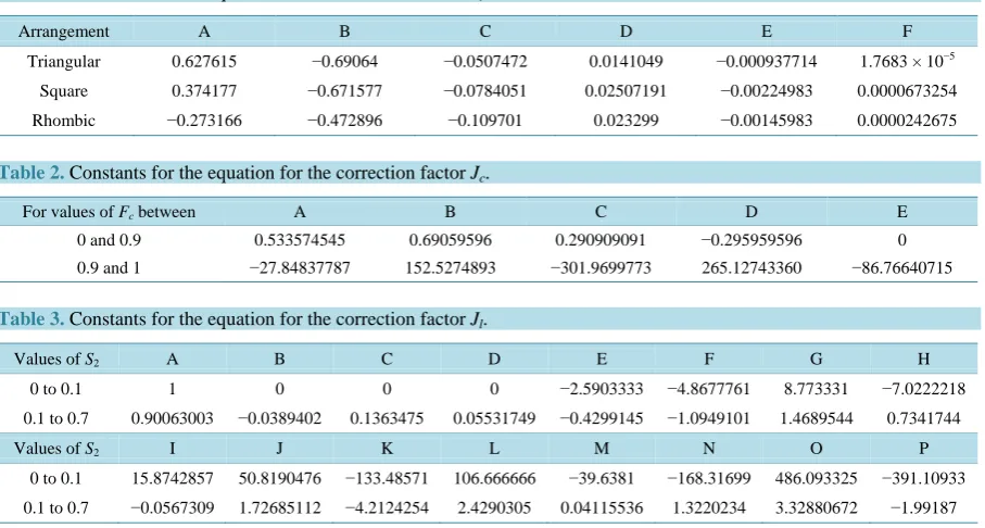
Table 1.Constants for the equation for the correction factor Ji.

Arrangement A B C D E F

Triangular 0.627615 −0.69064 −0.0507472 0.0141049 −0.000937714 1.7683 × 10−5

Square 0.374177 −0.671577 −0.0784051 0.02507191 −0.00224983 0.0000673254

Rhombic −0.273166 −0.472896 −0.109701 0.023299 −0.00145983 0.0000242675

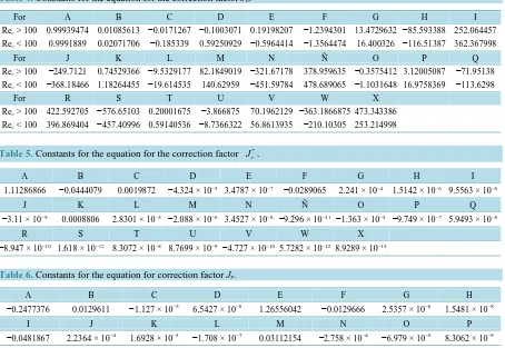
Table 2. Constants for the equation for the correction factor Jc.

For values of Fc between A B C D E

0 and 0.9 0.533574545 0.69059596 0.290909091 −0.295959596 0

0.9 and 1 −27.84837787 152.5274893 −301.9699773 265.12743360 −86.76640715

Table 3. Constants for the equation for the correction factor Jl.

Values of S2 A B C D E F G H

0 to 0.1 1 0 0 0 −2.5903333 −4.8677761 8.773331 −7.0222218

0.1 to 0.7 0.90063003 −0.0389402 0.1363475 0.05531749 −0.4299145 −1.0949101 1.4689544 0.7341744

Values of S2 I J K L M N O P

0 to 0.1 15.8742857 50.8190476 −133.48571 106.666666 −39.6381 −168.31699 486.093325 −391.10933

2.4. Correction Factor by Recirculation Flow Effect, Jb

The recirculation currents do not exchange heat through the tubes and this issue is considered by the correction factor Jb. This factor is computed by Equation (8) which is based on Fsbp. The constant of the Equation N2 = Nss/Nc are defined in Table 4 in terms of Rec.

( )

( )

( )

( )

( )

( )

( )

( )

( )

( )

( )

( )

( )

( )

( )

( )

( )

( )

( )

( )

2 3 4 2 3 4

2 2 2 2 2 2 2 2

2 3 4 2 2 3 4 3

2 2 2 2 2 2 2 2

2 3 4 4

2 2 2 2

A B C D E F G H I J

K L M N O P Q R S

T U V W X

b sbp

sbp sbp

sbp

J N N N N N N N N F

N N N N F N N N N F

N N N N F

   

=_ + + + + _{ }+ + + + + _

   

+_ + + + + Ν _ +_ + + + + _

 

+_ + + + + _

 (8)

A maximum error of 1.3% is result of comparing the original graph against that one obtained by Equation (8).

2.5. Correction Factor by Adverse Temperature Gradient Jr

This factor has the value of 1 if Rec ≥ 100. When Rec fluctuation is between 0 and 100, the next criterion is used: 1) If Rec ≤ 20, Jr will acquire the same value as J*r using the Equation (9), and knowing that Nb and N1 = Nc + Ncw are constants which are shown in Table 5.

( )

( )

( )

( )

( )

( )

( )

( )

( )

( )

( )

( )

( )

( )

( )

( )

( )

( )

( )

( )

2 3 4 2 3 4

*

1 1 1 1 1 1 1 1

2 3 4 2 2 3 4 3

1 1 1 1 1 1 1 1

2 3 4 4

1 1 1 1

A B C D E F G H I J

K L M N O P Q R S

T U V W X

r b

b b

b

J N N N N N N N N N

N N N N N N N N N N

N N N N N

   

=_ + + + + _{ }+ + + + + _

   

+_ + + + + Ν _ +_ + + + + _

 

+_ + + + + _

 (9)

A maximum error of 1.9% is result of comparing the original graph against that one obtained by Equation (8). 2) If 20 ≤ Rec ≤ 100, Jr is computed by Equation (10) which depends on Jr*, Rec and Table 6 constants.

Table 4. Constants for the equation for the correction factor Jb.

For A B C D E F G H I

Rec > 100 0.99939474 0.01085613 −0.0171267 −0.1003071 0.19198207 −1.2394301 13.4729632 −85.593388 252.064457

Rec < 100 0.9991889 0.02071706 −0.185339 0.59250929 −0.5964414 −1.3564474 16.400326 −116.51387 362.367998

For J K L M N Ñ O P Q

Rec > 100 −249.7121 0.74529366 −9.5329177 82.1849019 −321.67178 378.959635 −0.3575412 3.12005087 −71.95138

Rec < 100 −368.18466 1.18264455 −19.614535 140.62959 −451.59784 478.689065 −1.1031648 16.9758369 −113.6298

For R S T U V W X

Rec > 100 422.592705 −576.65103 0.20001675 −3.866875 70.1962129 −363.1866875 473.343386

Rec < 100 396.869404 −457.40996 0.59140536 −8.7366322 56.8613935 −210.10305 253.214998

Table 5. Constants for the equation for the correction factor *

r

J .

A B C D E F G H I

1.11286866 −0.0444079 0.0019872 −4.324 × 10−5 3.4787 × 10−7 −0.0289065 2.241 × 10−4 1.5142 × 10−6 9.5563 × 10−8

J K L M N Ñ O P Q

−3.11 × 10−9 _{0.0008806 2.8301 × 10}−5 _{−2.088 × 10}−6 _{3.4527 × 10}−8 _{−9.296 × 10}−11 _{−1.363 × 10}−5 _{−9.749 × 10}−7 _{5.9493 × 10}−8

R S T U V W X

−8.947 × 10−10 _{1.618 × 10}−12 _{8.3072 × 10}−8 _{8.7699 × 10}−9 _{−4.727 × 10}−10 _{5.7282 × 10}−12 _{8.9289 × 10}−15

Table 6. Constants for the equation for correction factor Jr.

A B C D E F G H

−0.2477376 0.0129611 −1.127 × 10−5 6.5427 × 10−8 1.26556042 −0.0129666 2.5357 × 10−6 1.5481 × 10−8

I J K L M N O P

(

) (

)

(

)

(

)

2 3 2 3 *

2 3 *2 2 3 *3

Re Re Re Re Re Re

Re Re Re Re Re Re

r c c c c c c r

c c c r c c c r

J A B C D E F G H J I J K L J M N O P J

= + + + + + + +

+ + + + + + + + (10)

In the previous equation, J*r is calculated by Equation (9). Comparing both graphics, the original and that one obtained by Equation (10), it is observed as maximum error 3.8%.

2.6. Correction Factor by Uneven Baffle Spacing at the Inlet and/or Outlet, Js

This factor has an effect when exist a different baffle distribution at the inlet and/or outlet and along the tube bundle and it is computed by Equation (11):

(

)

( )

( )

(

)

b s I s o

s

b s I s o

N l l J

N l l

′′ ′′ − −

− + +

=

− + + (11)

where n′′ = 0.6 for turbulent flow and (Rec > 100).

n′′ = 1/3 for laminar flow and (Rec < 100).

2.7. Correction Factor by Friction of an Ideal Bank Tubes fi

The correction factor by friction in a triangular and rotated square set is determined in function of Rec and the constants presented in Table 7 by the Equation (12).

(

)

(

)

(

)

(

)

(

)

{

(

)

(

)

(

)

(

)

}

2 3 4 5

6 7 8 9

exp A B ln Re C ln Re D ln Re E ln Re F ln Re

G ln Re H ln Re I ln Re J ln Re

i c c c c c

c c c c

f = + + + + +

+ + + + (12)

A maximum error of 4.9% is result of comparing the original graph to that one obtained by Equation (12).

2.8. Pressure Loss Correction Factor by Tube-Baffle Leakage Rl

The introduction of this correction factor is due to the leakage of the tube bundle and it is computed by Equation (13) which is in terms of S1 =Ssb

(

)

(

)

( )

( )

( )

( )

( )

( )

( )

( )

( ) ( )

( )

( )

( ) ( )

2 3 2 3

1 1 1 1 1 1 2

2 3 2 2 3 3

1 1 1 2 1 1 1 2

A B C D E F G H

I J K L M N O P

l

R S S S S S S S

S S S S S S S S

   

=_ + + + _{ }+ + + + _

   

+ +_ + + _ +_ + + + _ (13)

The constants required by the equations are established in Table 8. Comparing the original graph and that one obtained by Equation (13) is observed a maximum error of 4.5%.

Table 7. Constants for the equation for the correction factor fi.

Type arrangement, outside diameter and pitch between tubes

A B C D E

Arrangement Diameter Pitch

Triangular 19.05 mm 23.8125 mm 4.15076 −0.675323 −0.254615 0.0590471 −0.00431448 Triangular 25.4 mm 31.75 mm 4.15076 −0.675323 −0.254615 0.0590471 −0.00431448

Rhombic 19.05 mm 25.4 mm 3.69311 −1.18662 0.281179 −0.136488 0.0280708

Triangular 19.05 mm 25.4 mm 3.85004 −0.609235 −0.278939 0.0630913 −0.00452036

Rhombic 25.4 mm 31.75 mm 3.97656 −0.796179 −0.1565 0.0319655 −0.00143937

Square 19.05 mm 25.4 mm 3.76203 −0.9323 −0.0827537 0.0678788 −0.0281861

Square 25.4 mm 31.75 mm 3.99352 0.768721 −0.32634 0.176985 −0.0326325

Type arrangement, outside diameter and pitch between tubes

F G H I J

Arrangement Diameter Pitch

Triangular 19.05 mm 23.8125 mm 0.000102933 0 0 0 0

Triangular 25.4 mm 31.75 mm 0.000102933 0 0 0 0

Rhombic 19.05 mm 25.4 mm −0.00237654 0.0000713989 0 0 0

Triangular 19.05 mm 25.4 mm 0.000103903 0 0 0 0

Rhombic 25.4 mm 31.75 mm 0.00547024 −0.000459287 0.000013822 0 0

Table 8. Constants for the equation for the correction factor Rl.

Values of S1 A B C D E F G H

0 to 0.3 0.9930511 0.04163241 −0.07862612 0.01413662 −4.092978 −6.546514 4.516072 −2.525205

0.3 to 0.8 0.7499537 −0.4381533 0.2981431 0.1471556 −0.709333 0.0847061 1.053554 −4.215857

Values of S1 I J K L M N O P

0 to 0.3 15.6087 30.3289 −23.86598 14.08358 −23.22663 −41.67332 24.92778 −15.50438

0.3 to 0.8 0.3060496 1.27137 −12.85256 19.67211 −0.212271 −3.186438 18.491314 −23.16708

2.9. Pressure Loss Correction Factor by Recirculation Effect Rb

This correction factor is provoked by circulation currents in the heat exchanger and it is computed by Equation (14) which is in terms of Fsbp and N2 = Nss/Nc.

( )

( )

( )

( )

( )

( )

( )

( )

( )

( )

( )

( )

( )

( )

( )

( )

( )

( )

( )

( )

2 3 4 2 3 4

2 2 2 2 2 2 2 2

2 3 4 2 2 3 4 3

2 2 2 2 2 2 2 2

2 3 4 ₄

2 2 2 2

A B C D E F G H I J

K L M N O P Q R S

T U V W X

b sbp

sbp sbp

sbp

R N N N N N N N N F

N N N N F N N N N F

N N N N F

+

   

=_ + + + + _{ }+ + + + + _

   

+_ + + + + Ν _{ } + + + + _

 

+_ + + + + _

 (14)

The constants demanded by the equation are defined in Table 9 and they are in terms of Rec number. Com- paring the original graph and that one obtained by Equation (14), the maximal error found is 1.3%.

2.10. Pressure Loss Correction Factor by Uneven Baffle Spacing at the Inlet and Outlet

This correction factor is proposed by the uneven baffle spacing at inlet and outlet of the heat exchanger and this factor is calculated by Equation (15).

( ) ( )

, ,

1 2

n n

s s I s o

R = _ l −′+ l −′_

  (15)

where n′ = 1.6 for turbulent flow (Rec > 100).

n′ = 1 for laminar flow (Rec < 100).

3. Calculus Program

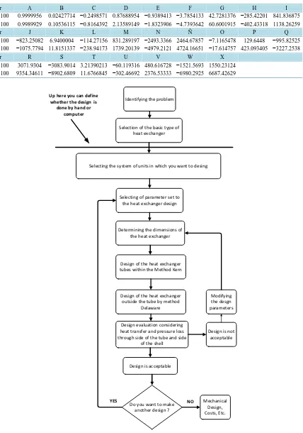
Having the correction factors in an analytical form, it was developed a calculus program using the FORTRAN 77 language which will design quickly the shell and tubes heat exchanger through the improvement DELAWARE Method. This computing program is described next:

Flow Chart Program

The flow chart used for the shell and tubes heat exchanger is presented in Figure 2.

As from this flow chart, it was made the heat exchanger design program using the executable BELL since it runs in MS DOS platform.

4. Conclusions

This work has presented the improvements to the Delaware method for the shell and tube heat exchanger design. These improvements were made up not only of obtaining the correction factor equations which were only avail- able in graphic forma but also of developing the computing program in Fortran 77 language.

Thus, a new and easy tool for the shell and tubes heat exchanger design is available which allows accom- plishing the numerical computing in a quick form minimizing the errors of the graphical lecture. This system gives the opportunity to explore different design alternatives in order to find the optimal solution to each pro- posed problem.

Table 9. Constants for the equation for the correction factor Rb.

For A B C D E F G H I

Rec > 100 0.9999956 0.02427714 −0.2498571 0.87688954 −0.9389413 −3.7854133 42.7281376 −285.42201 841.836875

Rec < 100 0.9989929 0.10536115 −0.8164392 2.13589149 −1.8323906 −4.7393642 60.6001915 −402.43318 1138.26259

For J K L M N Ñ O P Q

Rec > 100 −823.25082 6.9400004 −114.27156 831.289197 −2493.3366 2464.67857 −7.1165478 129.6448 −995.82525

Rec < 100 −1075.7794 11.8151337 −238.94173 1739.20139 −4979.2121 4724.16651 −17.614757 423.093405 −3227.2538

For R S T U V W X

Rec > 100 3071.9304 −3083.9014 3.21390213 −60.119316 480.616728 −1521.5693 1550.23124

Rec < 100 9354.34611 −8902.6809 11.6766845 −302.46692 2376.53333 −6980.2925 6687.42629

Figure 2. Flow chart program.

Up here you can define whether the design is

done by hand or computer

Identifying the problem

Selection of the basic type of heat exchanger

Selecting the system of units in which you want to desing

Selecting of parameter set to the heat exchanger design

Determining the dimensions of the heat exchanger

Design of the heat exchanger tubes within the Method Kern

Design of the heat exchanger outside the tube by method

Delaware

Design evaluation considering heat transfer and pressure loss through side of the tube and side

of the shell

Design is not acceptable

Modifying the desgn parameters

Design is acceptable

Do you want to make another design ?

Mechanical Design, Costs, Etc.

tube heat exchanger design.

References

[1] Vengateson, U. (2010) Design of Multiple Shell and Tube Heat Exchangers in Series: E Shell and F Shell. Chemical Engineering Research and Design, 88, 725-736. http://dx.doi.org/10.1016/j.cherd.2009.10.005

[2] Costa, A.L.H. and Queiroz, E.M. (2008) Design Optimization of Shell and tube Heat Exchangers. Applied Thermal Engineering, 28, 1798-1805. http://dx.doi.org/10.1016/j.applthermaleng.2007.11.009

[3] Serna, M. and Jimenez, A. (2005) A Compact Formulation of Bell-Delaware Method for Heat Exchanger Desing and Optimation. Chemical Engineering Research and Desing, 83, 539-550. http://dx.doi.org/10.1205/cherd.03192

[4] Shah, R.K., Dusan, P. and Sekulic, D.P. (2003) Fundamentals of Heat Exchanger Design. John Wiley & Sons, Hobo- ken. http://dx.doi.org/10.1002/9780470172605

[5] Ayub, Z.H. (2005) A New Chart Method for Evaluating Single-Phase Shell Side Heat Transfer Coefficient in a Single Segmental Shell and Tube Heat Exchanger. Applied Thermal Engineering, 25, 2412-2420.

http://dx.doi.org/10.1016/j.applthermaleng.2004.12.015

[6] Leong, K.C., Toh, K.C. and Leong, Y.C. (1998) Shell and Tube Heat Exchanger Design Software for Educational Ap- plications. International Journal of Engineering Education, 14, 217-224

[7] León, A.R., Velazquez, M.T. and Diez, P.Q. (2011) The Design of Heat Exchangers. Engineering, 3, 911-920. [8] Castillo, R. (1999) Diseño Computacional de Intercambiadores de Calor de Coraza y Tubos por el Método Delaware.

Nomenclature

ρc Fluid density.

μc Average fluid viscosity.

∆Pb,i Pressure loss in a cross-flow section. ∆Pc Total pressure loss on the side of the shell. ∆Pw,i Pressure loss in a window section.

μwc Fluid Viscosity wall temperature.

A Heat transfer area.

Cpc Specific heat.

et Tube thickness.

Fc Total fraction of tubes in cross flow.

F Correction factor heat exchanger configuration.

fi Correction factor due to friction.

Fsbp Fraction cross flow area available for recirculation flow.

g Acceleration of gravity.

hcc Fluid convection coefficient outside the tubes.

hio Convection coefficient of the fluid by the tube side.

r

J∗ Basic correction factor for adverse effect of the temperature gradient.

Jb Correction factor recirculation effect.

Jc Effect correction factor baffle configuration.

Ji Correction factor due to friction.

Jl Correction factor for leakage effect.

Jr Correction factor adverse effect of the temperature gradient.

Js Correction factor for baffle uneven spacing effect on entry and exit.

k Thermal conductivity of the tube material.

kc Thermal conductivity of the fluid.

* *

, , , ,

s o s I s o s s I s l =l =l l =l l

ls Spacing between baffles.

ls,I, ls,o Spacing of baffles at the entrance and exit.

Nb Number of baffles.

Nc Number of rows in cross flow section.

Ncw Number of rows in section window.

Nss Numbers Stamp/sides sealed.

Nt Number of tubes.

Q Heat flux exchanged.

Rb Correction factor recirculation effect.

Rd Total coefficient of fouling.

Rec Reynolds number.

Rl Correction factor for leakage effect.

Rs Correction factor adverse effect of the temperature gradient.

Ssb Correction factor for baffle uneven spacing effect on entry and exit.

Stb Thermal conductivity of the tube material.

Tmlc Thermal conductivity of the fluid.

Udc Spacing between baffles.