5
X
October 2017
Optimum Parameters for Fault Detection in
Bioreactor Using Support Vector Machine and
Neural Network
Mr. Rahul Shrivastava1 Dr. Hari Mahalingam2, Prof. NN Dutta3
1
Department of Chemical Engineering, Jaypee University of Engineering and Technology, AB-road, Raghogarh, Guna (MP), INDIA-473226.
2
Department of Chemical Engineering National Institute of Technology Karnataka, Surathkal, INDIA-575025. 3
Department of Chemical Engineering, Jaypee University of Engineering and Technology, AB-road, Raghogarh, Guna (MP), INDIA-473226.
Abstract: Bioprocesses are parameter sensitive, highly non-linear and complex in nature. Apart from close monitoring of the process variables and good control strategy, a robust fault detection and diagnosis (FDD) strategy will help in maintaining the quality of the product by early detection of fault. This paper discusses the application of support vector machines (SVM) and artificial neural networks (ANN) in classifying the normal and faulty conditions in semi-batch bioreactor for penicillin production. The SVM classifier was implemented with three kernel functions viz. linear, polynomial and Gaussian radial basis function (RBF). In case of ANN, a back propagation two layer feed forward neural network was used. The optimum SVM and ANN models were found when the model produced the minimal error with respect to the training, testing and data validation. In case of SVM, it was found that linear kernel is not suitable for bioreactor data, whereas RBF outperformed the polynomial function. Further the performance of SVM was compared with ANN, and ANN outperformed SVM.
Keyword: fault detection, bioreactor, support vector machine, artificial neural network.
I. INTRODUCTION
In order to achieve maximum productivity, to reduce product rejection rate and to satisfy safety and environmental regulations there has been great interest in the development of FDD methods. In past decades, Different methods have been developed to detect and diagnose faults in complex systems. FDD approaches can be roughly divided into two major categories: model based methods and process history based methods. Model based methods make use of the quantitative/qualitative models. Quantitative models are based on first principles of a physical system and qualitative models are based on the available information and knowledge of a physical system [1, 2]. On the other hand, process history based methods require large amount of historical data, which contain the typical trends and previous fault information for effective monitoring methods to be built [3]. Generally, the model-based methods are more accurate, provided that the exact mathematical model is available. However, it is difficult to develop the mathematical model for a process which is complex and highly non-linear in nature. For such processes, process history based methods are found to be more successful than model-based methods. In the last decade the researchers have extensively used process history based methods for studies such as [4-6] for ANN and [7-9] for SVM.
The article is organized as follows. The section.2 contains the brief description of SVM and ANN, and proposed method is also representing in this section. Section.3 presents the dataset description. Section.4 is result and discussion section, where the fault classifier were constructed, trained and tested for performance comparison. Finally, conclusion was drawn in section.5.
II. THEORY& METHODS
A. Support vector machines (SVM)
SVM were introduced by Bose ret al [13]. SVM are based on the Structural Risk Minimization principle from the Statistical Learning Theory [14]. SVM are basically binary classification methods, which separates the negative instances from positive ones by learning a maximum margin linear hyperplane between them.
. + ≤ −1
. + = 0
[image:3.612.111.374.220.427.2]. + ≥+1
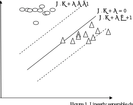
Figure 1. Linearly separable data
See Fig.1, a series of data points for two different classes are shown. Negative and positive classes are represented by ovals and triangles respectively. A linear boundary between the two different classes is placed. Furthermore, SVM orients the boundary in such a way that the distance between the boundary and the nearest data point in each class is maximal. The nearest data points that used to define the margin are called support vectors.
The linear classifier is defined by two elements: a weight vector w (with one component for each feature), and a bias . The classification rule assigns +1, to a new example x, when ( ) = . + ≥ 0, and −1 otherwise.
In order to implement support vector machine classifier, margin between the samples has to be maximized, i.e.
| |. The formulation
of SVM will be as follow
Minimize ||w||2− − − − − − − − − − − − − − − − − − − − − −(1)
Subject to constraint ( . + ) − 1 ≥ 0 ∀ − − − − − − − − − −(2)
This is primal formulation of linear SVM, which is a convex quadratic optimization problem. Further, this problem can be recast into dual form, by using Lagrange multiplier. One can refer Burges [15] for detailed description of the derivation.
Maximize ∑ − ∑ ∑ . − − − − − − − − − − −(3)
Subject to: ≥0 and ∑ = 0− − − − − − − − − − − −(4)
Then the vector w is defined in terms of : =∑ − − − − − − − − − −(5)
Figure 2. Slightly non-linear data
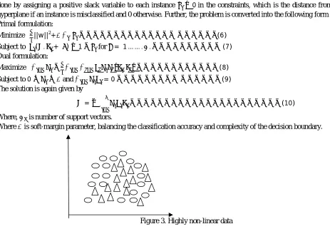
This problem is resolved by allowing a few anomalous data points to fall on the wrong side of the separating hyperplane. This is done by assigning a positive slack variable to each instance ≥0 in the constraints, which is the distance from the separating hyperplane if an instance is misclassified and 0 otherwise. Further, the problem is converted into the following form
Primal formulation:
Minimize ||w||2+ ∑ − − − − − − − − − − − − − − − − − − − −(6)
Subject to ( . + )≥1− for = 1 … … . .− − − − − − − − − − (7)
Dual formulation:
Maximize ∑ − ∑ ∑ . − − − − − − − − − − − − (8)
Subject to 0≤ ≤ and ∑ = 0− − − − − − − − − − − − − − −(9)
The solution is again given by
= − − − − − − − − − − − − − − − − − − − − − − (10)
Where, is number of support vectors.
Where is soft-margin parameter, balancing the classification accuracy and complexity of the decision boundary.
Figure 3. Highly non-linear data
[image:4.612.45.508.354.675.2]mainly on the parameters of kernel functions and the soft-margin parameter . See Christianini and Shawe-Taylor [16]for details about soft margin and non-linear SVM.
In practice, various kernel functions such as linear, polynomial, radial basis and sigmoid are used. Linear kernel function:
, = . − − − − − − − − − − − − − − − (11)
Polynomial kernel function:
, = ( . + 1) − − − − − − − − − − − − − (12)
is order of polynomial. On using high values of , there may be a problem of generalization due to over fitting. Value of must be selected carefully.
RBF kernel function:
, = exp (−|| − || /2σ )− − − − − − − − − (13)
Sigmoid kernel function:
, = tanh [ . + ]− − − − − − − − − − −(14)
In our analysis, we have used linear, polynomial and RBF kernel
B. Artificial neural network (ANN)
Several neural network architectures and learning algorithm have been proposed over the years [17]. We are just giving the brief description of feed forward ANN with back propagation algorithm. The ANN can be based on supervised and unsupervised learning. Feed forward network with back propagation belongs to supervised learning category.
Hidden layer
Input layer WCF Output layer
WAC
WCG
WAD WDF
WBC WDG
WBD WEF
WAE
[image:5.612.124.431.361.518.2]WBE WEG
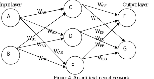
[image:5.612.144.495.614.716.2]Figure 4. An artificial neural network
Fig.4 is showing the simplest form of feed forward network. In feed forward networks, information flows in one way only i.e. from input to output units, in a feed forward direction. A neural network consists of three layers, i.e. input, hidden and output layer. The process; whereas the output layer consists of output nodes i.e. number of outputs/classes in the process. The hidden layer consists of a certain number of nodes, however, the appropriate numbers of hidden nodes cannot be known in advance. A multilayer network can also be used, which has more than one hidden layer. Fig.5 shows a simple artificial neural network, consisting of a single neuron.
Weights
Threshold
Inputs
0 or 1 Output
Figure 5. Artificial neural network consist of single neuron
C
F A
D
G B
E
Referring to the Fig.4 and Fig.5, output from the network can be given as follow
= ( − )− − − − − − − − −(15)
Where, is activation result, is function of perceptron learning algorithm, whereas , and are weight vector, input vector and target value respectively.
Between the input, output and hidden layers, there are layers of weights that serve as a connection between them. There are various methods to set the strengths of the connections exist. One way is to set the weights explicitly, using a priori knowledge. Another way is to train the neural network by feeding it teaching patterns and letting it change its weights according to some learning rule (supervised learning). In case of supervised learning, network is supplied with given set of input data together with desired set of output data (target values), one for each node, at the output layer. Actual output from the network must be matched with the desired output, if any discrepancy is found, then the weights are updated by prevailing learning rule until actual output from the network does not become equal to the desired output. Another method for training the network is known as unsupervised learning, where output are not available but network learn on its own by discovering and adapting to the structural features in the input patterns. In case of supervised learning, the difference between actual output and desired output can be minimized by using different methods like least absolute deviation, asymmetric least squares, percentage differences, least fourth powers and sum of the squared errors. Sum of the squared error is most common.
The backpropagation technique is employed as a way of reducing error in the network’s classification. The calculated error propagates back through the network for reduction. Inputs are propagated to the first layer of hidden units, whose output is calculated and propagated to the next hidden layer. This process is repeated until the output layer is reached. Each output layer unit calculates the activation, from the sum of weighted inputs from previous layers. The error on the desired output is computed and propagated back to the first hidden layer, where the weight matrix is updated. This process is repeated until the error is minimized as much as possible.
Suppose we are given a training set{( , ). . . ( , )}, Consisting of r ordered pairs of n- and m-dimensional vectors, which are called the input and output patterns. Let the primitive functions at each node of the network be continuous and differentiable. The weights are initialized randomly. When the input pattern from the training set is presented to the network, the network will produce an output , which is compared with target value . Our objective is to make and identical for = 1. . . , by using a learning algorithm. More precisely, we want to minimize the error function of the network. The error function is defined as follow
=1
2 ||o −t || − − − − − − − − − − − −(16)
Where, o represent the output from the network and t represents the actual target for a given input. The gradient of the error function is computed and used to correct the initial weights. Our task is to compute this gradient recursively. is actually the summation of square of all the errors, i.e. error for each element of input-output data.
The weights in the network are modified each time to make the error as low as possible. is a continuous and differentiable function of the ` weights , , . . . , ` in the network. We can thus minimize by using an iterative process of gradient descent, for which we need to calculate the gradient
= ( , , … … , ) − − − − − − − − − − − − (17)
Weights are updated by using the following increment
∆ =− = 1, … , − − − − − − − − − − − (18)
In our analysis, we have used the most popular form of neural network i.e. two layer feed forward network, which has only one hidden layer.
III. DATASET DESCRIPTION
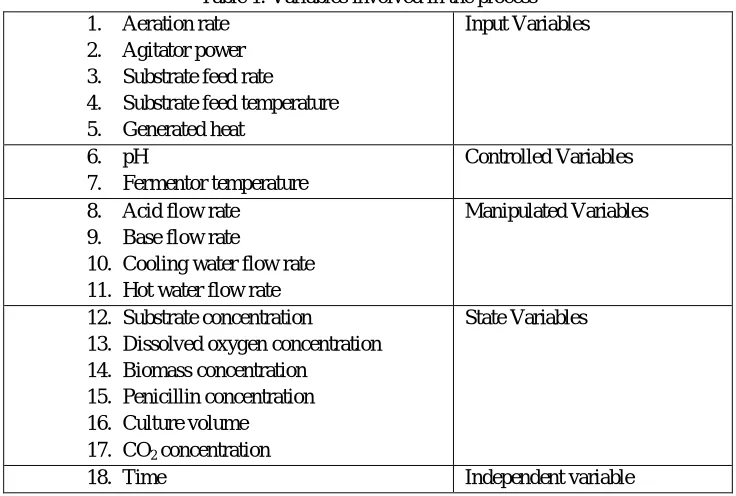
Table 1. Variables involved in the process 1. Aeration rate
2. Agitator power 3. Substrate feed rate 4. Substrate feed temperature 5. Generated heat
Input Variables
6. pH
7. Fermentor temperature
Controlled Variables
8. Acid flow rate 9. Base flow rate
10. Cooling water flow rate 11. Hot water flow rate
Manipulated Variables
12. Substrate concentration
13. Dissolved oxygen concentration 14. Biomass concentration
15. Penicillin concentration 16. Culture volume 17. CO2 concentration
State Variables
18. Time Independent variable
Out of the variables listed in Table 1, only 16 were used for analysis. The variables excluded were the time step and hot water flow rate; because time is an independent variable and hot water flow rate has zero value throughout the process.
[image:7.612.65.549.463.548.2]The PENSIM simulator provides for introduction of two fault types like step change and ramp change, which can be given to three variables namely aeration rate, agitator power and substrate feed rate. The first simulation was done for normal operation with default settings and then for four different faulty conditions by providing a step change of magnitude ±10% to aeration rate and agitator power. If anyone of these two variables goes beyond ±10% of their normal value, it indicates a fault. See Table 2 for the details of faults employed in this study.
Table 2. Summary of five simulations
S.No. Faulty variable Type of fault Magnitude
1. Normal operation No No
2. Aeration rate Step change +10%
3. Aeration rate Step change -10%
4. Agitator power Step change +10%
5. Agitator power Step change -10%
All the simulations were done for 150 h with a time interval of 0.25 h, thus generating 600 samples for normal and each faulty condition. A total of 3000 samples were generated and used for analysis, out of which 600 belongs to the class of normal operation and rest belong to the class of faulty condition. In addition to these 3000 samples, 1123 more samples were generated randomly for the normal and faulty conditions separately for testing purposes.
IV. RESULTS AND DISCUSSION
minimal optimization technique was used to find the optimal separating hyperplane. All the SVM models were trained using 5-fold cross validation. Search for the best parameters values was done for the following sets of values: ∈{1E-05,… ,1E+05} in each case and ∈{1E-04,…..,1E+04} for RBF kernel. The same dataset was studied with a feed forward ANN with back propagation. All the results were produced using MATLAB.
Table 3. Linear kernel
C
Misclassification error with training samples
(%) Time (s) Misclassification error with testing samples (%)
1.00E-05 36.7 5.1094 33.03
1.00E-04 33.73 5.4531 34.82
1.00E-03 35.33 5.1875 37.67
1.00E-02 45.7 5.8125 55.03
1.00E-01 46.87 9.1719 42.74
1 46.47 25.1719 56.09
1.00E+01 47.47 402.2188 55.65
1.00E+02 not converging
1.00E+03 not converging
1.00E+04 not converging
1.00E+05 not converging
[image:8.612.69.556.141.358.2]From Table 3, it can be observed that the bioreactor data is not separable by using linear SVM. For any value of , either the algorithm is not converging or if it converges, the misclassification error with training and testing samples is too high.
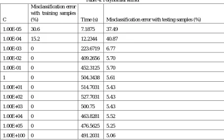
Table 4. Polynomial kernel
C
Misclassification error with training samples
(%) Time (s) Misclassification error with testing samples (%)
1.00E-05 30.6 7.1875 37.49
1.00E-04 15.2 12.2344 40.87
1.00E-03 0 223.6719 6.77
1.00E-02 0 409.2656 5.70
1.00E-01 0 452.3125 5.70
1 0 504.3438 5.61
1.00E+01 0 514.7031 5.43
1.00E+02 0 527.7031 5.43
1.00E+03 0 500.75 5.43
1.00E+04 0 463.8281 5.52
1.00E+05 0 476.5625 5.25
1.00E+100 0 491.2031 5.06
[image:8.612.78.533.413.699.2]misclassification error with testing samples is also very low, in the range of 5.06% to 6.77%. The training time is in the range from 7 to 527 seconds.
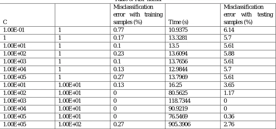
Table 5. RBF kernel
C σ
Misclassification error with training
samples (%) Time (s)
Misclassification error with testing samples (%)
1.00E-01 1 0.77 10.9375 6.14
1 1 0.17 13.3281 5.7
1.00E+01 1 0.1 13.5 5.61
1.00E+02 1 0.23 13.6094 5.88
1.00E+03 1 0.1 13.7656 5.61
1.00E+04 1 0.13 12.9844 5.7
1.00E+05 1 0.27 13.7969 5.61
1.00E+01 1.00E+01 0.13 16.25 3.65
1.00E+02 1.00E+01 0 80.5625 1.17
1.00E+03 1.00E+01 0 118.7344 0
1.00E+04 1.00E+01 0 90.9219 0
1.00E+05 1.00E+01 0 76.5469 0.36
1.00E+05 1.00E+02 0.27 905.3906 2.76
[image:9.612.67.546.111.336.2]Table 5 presents the results for RBF kernel. The best combinations of and are mentioned, rests are provided in the appendix. At some of the combinations of and values, the SVM models were producing nil misclassification error with training and testing samples. Training time is also low as compared to polynomial function.
Table 6. Feed forward ANN with back propagation
No. of neurons Time (s)
Misclassification error with training samples (%)
Misclassification error with testing samples (%)
10 4 0 0
15 5 0 0
20 8 0 0
25 6 0 0
50 10 0 0
100 24 0 0
See Table 6 for the performance of feed forward ANN with backpropagation. A 2-layer feed forward neural network with sigmoid hidden and output nodes was used. Mean squared error was used as a performance function. Input layer consists of 16 nodes, because there are 16 variables in bioreactor. Second layer is actually the hidden layer, where the number of nodes can be varied by the user. The output from the network will be either 0 (no-fault) or 1 (fault). The network performance was observed by changing the number of neurons in the hidden layer. The network was performing well with any value of number of neurons with very little time required for training and nil misclassification error with training and testing samples.
V. CONCLUSION
In case of SVM, it is evident that linear kernel is not appropriate for bioreactor data. However, polynomial and RBF kernel functions are able to classify normal and faulty conditions in bioreactor, but RBF outperformed polynomial kernel function. So, the parameter tuning and Choice of kernel function is crucial for efficient classification.
a result of large amount of samples was used for training. ANN typically performs well, ifnumber of classes to be separated is small and large amount of samples are available for training.
REFERENCES
[1] V. Venkatasubramanian, R. Rengaswamy, K.Yin, S. N. Kavuri, “A review of process fault detection and diagnosis Part I: Quantitative model-based methods”, Computers and Chemical Engineering, vol. 27, pp. 293-311, 2003a.
[2] V. Venkatasubramanian, R. Rengaswamy, S. N. Kavuri, “A review of process fault detection and diagnosis Part-II: Qualitative models and search strategies”, Computers & chemical engineering, vol. 27, vol. 313-326, 2003b.
[3] V. Venkatasubramanian, R. Rengaswamy, K. Yin, S. N. Kavuri, “A review of process fault detection and diagnosis Part III: Process history based methods”, Computers & chemical engineering, vol. 27, pp. 327-346, 2003c.
[4] D. Ruiz, J. Nougues-Maria, Z. Calderon, A. Espuna, L. Puigjaner, “Neural network based framework for fault diagnosis in batch chemical plants”, Computers and Chemical Engineering, vol. 24, pp. 777-784, 2000.
[5] Y. Zhou, J. Hahn, M. S. Mannan, “Fault detection and classification in chemical processes based on neural networks with feature extraction”, ISA Transactions, vol. 42, pp. 651–664, 2003.
[6] S. Rajakarunakaran, P. Venkumar, D. Devaraj, K. S. P. Rao, “Artificial neural network approach for fault detection in rotary system”, Applied Soft Computing, vol. 8, pp. 740–748, 2008.
[7] A. Kulkarni, V. K. Jayaraman, B. D. Kulkarni, “Knowledge incorporated support vector machines to detect faults in Tennessee Eastman Process”, Computers and Chemical Engineering, vol. 29, pp. 2128-2133, 2005.
[8] I. Yélamos, G. Escudero, M. Graells, L. Puigjaner, “Fault diagnosis based on support vector machines and systematic comparison to existing approaches”, Computers & Chemical Engineering, vol. 21, pp. 1209-1214, 2006.
[9] I. Yélamos, G. Escudero, M. Graells, L. Puigjaner, “Simultaneous fault diagnosis in chemical plants using support Vector Machines”, Computers & Chemical Engineering, vol. 24, pp. 1253-1258, 2007.
[10] K. R. Patil, A. J. Kulkarni, “A Simple Visualization Techniqueto Understand the System Dynamics in Bioreactors”,Biotechnology Progress, vol. 23, pp. 1101-1105, 2007.
[11] R. Krishna, S. Nanda, A. Kulkarni, S. Patil, “A partial Granger causality based method for analysis of parameter interactions in bioreactors” Computers and Chemical Engineering, vol. 35, pp. 121-126, 2011.
[12] G. Birol, C. Undey, A. Cinar, “A modular simulation package for fed batch fermenation: Penicillin production. Computers & Chemical Engineering”, vol. 26(11), pp. 1553–1565, 2002.
[13] B. Boser, I. Guyon, V. Vapnik, “A training algorithm for optimal margin classifiers”, In Proceedings of fifth annual workshop on computational learning theory, COLT, New York, USA, pp. 144-152, 1992..
[14] V. N. Vapnik, “Statistical learning theory”, John Wiley, 1998.
[15] C. J. C. Burges, “A tutorial on support vector machines for pattern identification” Daa Mining and Knowledge Discovery, vol. 2, pp. 121–167, 1998. [16] N. Christianini, J. Shawe-Taylor, “An introduction to suppot vector machines”, Cambridge University Press, 2000.
[17] J. A. Anderson, “An introduction to neural networks”, MIT Press, 1995.
.
APPENDEX
Remaining results for RBF kernel from Table 5.
C σ
Percent error with
training samples Time (s) Percent error with testing samples
1.00E-05 1 4.7 10.0156 11.75
1.00E-04 1 4.87 10.4063 16.21
1.00E-03 1 4.37 10.5156 12.73
1.00E-02 1 4.67 10.3125 14.16
1.00E-05 1.00E+01 34.73 8.9844 35.17
1.00E-04 1.00E+01 33.7 8.625 31.79
1.00E-03 1.00E+01 33.47 9.0781 31.88
1.00E-02 1.00E+01 34.33 9.0625 39.63
1.00E-01 1.00E+01 40.4 8.7344 33.40
1 1.00E+01 39.7 8.8906 24.13
1.00E-05 1.00E+02 34.53 8.6094 33.21
1.00E-04 1.00E+02 37.23 8.5938 32.77
1.00E-02 1.00E+02 34.47 9.125 35.35
1.00E-01 1.00E+02 39.5 8.8281 33.21
1 1.00E+02 35.27 9.0625 32.24
1.00E+01 1.00E+02 34.83 9.2344 32.32
1.00E+02 1.00E+02 46.73 9.7031 37.49
1.00E+03 1.00E+02 46.7 12.2188 49.42
1.00E+04 1.00E+02 41.7 38.5 39.54
1.00E-05 1.00E+03 33.47 9.0781 38.47
1.00E-04 1.00E+03 35.63 8.8281 37.93
1.00E-03 1.00E+03 34.97 9.2813 40.34
1.00E-02 1.00E+03 34.47 8.75 32.95
1.00E-01 1.00E+03 34.53 8.5938 34.64
1 1.00E+03 34.53 8.6719 36.76
1.00E+01 1.00E+03 34.83 8.8125 33.04
1.00E+02 1.00E+03 34.23 8.9063 35.62
1.00E+03 1.00E+03 34.9 8.8281 36.24
1.00E+04 1.00E+03 45.4 9.2188 41.41
1.00E+05 1.00E+03 47.27 12.5625 55.83
1.00E-05 1.00E+04 34.33 8.8438 35.08
1.00E-04 1.00E+04 34.37 8.7188 33.75
1.00E-03 1.00E+04 33.97 8.6719 34.46
1.00E-02 1.00E+04 35.77 9.0469 35.62
1.00E-01 1.00E+04 35.07 8.8438 34.73
1 1.00E+04 34.13 8.7344 49.69
1.00E+01 1.00E+04 33.7 9.0469 47.55
1.00E+02 1.00E+04 34.43 8.6094 32.24
1.00E+03 1.00E+04 34.73 9.0938 33.93
1.00E+04 1.00E+04 34 8.9375 34.55
1.00E+05 1.00E+04 38.17 9.0625 43.37
1.00E-05 1.00E-01 17.9 10.7031 42.03
1.00E-04 1.00E-01 17.57 10.8594 42.03
1.00E-03 1.00E-01 17.57 11.1875 42.03
1.00E-02 1.00E-01 17.47 10.9531 42.30
1.00E-01 1.00E-01 17.6 11 42.30
1 1.00E-01 10.3 30.6719 39.27
1.00E+01 1.00E-01 10.1 30.9688 39.27
1.00E+02 1.00E-01 10.5 28.7344 40.07
1.00E+03 1.00E-01 10.53 28.3906 38.74
1.00E+04 1.00E-01 10 27.2969 39
1.00E+05 1.00E-01 9.97 29.2969 39.27
1.00E-05 1.00E-02 19.97 9.2031 42.39
1.00E-03 1.00E-02 20.2 8.8281 42.48
1.00E-02 1.00E-02 20.07 9.0469 42.48
1.00E-01 1.00E-02 19.97 9.1563 42.39
1 1.00E-02 19.97 28.4219 42.12
1.00E+01 1.00E-02 20.13 31.25 42.21
1.00E+02 1.00E-02 19.97 29.3281 42.12
1.00E+03 1.00E-02 19.97 30.0156 42.12
1.00E+04 1.00E-02 19.97 30.4531 42.12