Quantum and algorithmic Bayesian mechanisms

Munich Personal RePEc Archive

Quantum and algorithmic Bayesian

mechanisms

Wu, Haoyang

5 April 2011

Online at

https://mpra.ub.uni-muenchen.de/30072/

Quantum and algorithmic Bayesian mechanisms

Haoyang Wu

∗

Abstract

Bayesian implementation concerns decision making problems when agents have incom-plete information. This paper proposes that the traditional sufficient conditions for Bayesian implementation shall be amended by virtue of a quantum Bayesian mechanism. Further-more, by using an algorithmic Bayesian mechanism, this amendment holds in the macro world too.

1 Introduction

Mechanism design is an important branch of economics. Compared with game the-ory, it concerns a reverse question: given some desirable outcomes, can we design a game that produces them? Nash implementation and Bayesian implementation are two key parts of the mechanism design theory. The former assumes complete infor-mation among the agents, whereas the latter concerns incomplete inforinfor-mation. Ref. [1] is a seminal work in the field of Nash implementation. It provides an almost complete characterization of social choice rules that are Nash implementable when the number of agents is at least three. Palfrey and Srivastava [2], [3], and Jackson [4] together constructed a framework for Bayesian implementation.

In 2010, Wu [5] claimed that the sufficient conditions for Nash implementation shall be amended by virtue of a quantum mechanism. Furthermore, this amendment holds in the macro world by virtue of an algorithmic mechanism [6]. Given these accomplishments in the field of Nash implementation, this paper aims to investigate what will happen if the quantum mechanism is applied to Bayesian implementation.

The rest of this paper is organized as follows: Section 2 recalls preliminaries of Bayesian implementation given by Serrano [7]. In Section 3, a novel property, multi-Bayesian monotonicity, is defined. Section 4 and 5 are the main parts of this

paper, in which we will propose quantum and algorithmic Bayesian mechanisms respectively. Section 6 draws the conclusions.

2 Preliminaries

LetN = _{1,_{· · ·} ,n_}be a finite set ofagents withn _≥ 2, A= _{a1,· · · ,ak}be a finite

set of social outcomes. Let Ti be the finite set of agent i’s types, and the private

informationpossessed by agentiis denoted asti ∈Ti. We refer to a profile of types

t = (t1,· · · ,tn) as astate. Consider environments in which the statet = (t1,· · · ,tn)

is not common knowledge among the n agents. We denote byT the set of states compatible with an environment, i.e., a set of states that is common knowledge among the agents. LetT = Q_i∈NTi. Each agenti ∈ N knows his typeti ∈ Ti, but

not necessarily the types of the others. We will use the notationt₋ito denote (tj)j,_i.

Similarly,T₋i =Qj,_iTj.

Each agent has a prior belief, probability distribution, qi defined onT. We make

an assumption of nonredundant types: for every i _∈ N and ti ∈ Ti, there exists

t₋i ∈T−i such thatqi(t) > 0. For eachi ∈N andti ∈ Ti, the conditional probability

oft₋i ∈T−i, giventi, is theposterior belief of typeti and it is denotedqi(t−i|ti). Let

T∗ _⊆ T be the set of states with positive probability. Given agent i’s state ti and

utility functionui(·,t) : ∆×T 7→ R, theconditional expected utility of agenti of

typeti corresponding to a social choice function (SCF) f :T 7→ ∆is defined as:

Ui(f|ti)≡

X

t′ −i∈T−i

qi(t′₋i|ti)ui(f(t′₋i,ti),(t′₋i,ti)).

An environment with incomplete informationis a list E =< N,A,(ui,Ti,qi)i∈N >.

For simplicity, we shall consider only single-valued rules. An SCF f is a mapping

f :T _7→ A. Let_F denote the set of SCFs. Two SCFs f andhareequivalent(f _≈ h) if f(t)=h(t) for everyt_∈T∗_.

Consider amechanismΓ =((Mi)i∈N,g) imposed on an incomplete information

envi-ronmentE,g: M_{7→ F}. ABayesian Nash equilibriumofΓis a profile of strategies σ∗= (σ∗_i)i∈N whereσ∗_i :Ti 7→ Misuch that for alli∈N and for allti ∈Ti,

Ui(g(σ∗)|ti)≥Ui(g(σ∗₋i, σ′i)|ti), ∀σ′i :Ti 7→ Mi.

Denote by _B(Γ) the set of Bayesian equilibria of the mechanism Γ. Let g(_B(Γ)) be the corresponding set of equilibrium outcomes. An SCF f is Bayesian imple-mentableif there exists a mechanism Γ = ((Mi)i∈N,g) such thatg(B(Γ)) ≈ f. An

mechanism associated with f, i.e., if for everyi_∈N and for everyti ∈Ti,

X

t′_−i∈T−i

qi(t′₋i|ti)ui(f(t′₋i,ti),(t′₋i,ti))≥

X

t′_−i∈T−i

qi(t₋′i|ti)ui(f(t₋′i,t′i),(t′−i,ti)),

∀t_i′ _∈ Ti. Consider a strategy in a direct mechanism for agent i, i.e., a mapping

αi =(αi(ti))ti∈Ti :Ti 7→ Ti. Adeceptionα= (αi)i∈N is a collection of such mappings where at least one differs from the identity mapping. Given an SCF f and a decep-tionα, let [f _◦α] denote the following SCF: [f _◦α](t) = f(α(t)) for everyt _∈ T. For a type ti ∈ Ti, an SCF f, and a deception α, let fαi(ti)(t′) = f(t₋′i, αi(ti)) for all

t′ _∈T.

An SCF f isBayesian monotonicif for any deceptionα, whenever f _◦α0 _f, there existi_∈N,ti ∈Ti, and an SCFysuch that

Ui(y◦α|ti)>Ui(f ◦α|ti), whileUi(f|ti′)≥Ui(yαi(ti)|t

′

i), ∀t′i ∈Ti. (*).

According to Ref. [7], the sufficient and necessary conditions for Bayesian imple-mentation are incentive compatibility and Bayesian monotonicity. To facilitate the following discussion, here we cite the Bayesian mechanism (P404, Line 4, [7]) as follows: Consider a mechanism Γ = ((Mi)i∈N,g), where Mi = Ti × F ×Z+. Each

agent is asked to report his type ti, an SCF fi and a nonnegative integer zi, i.e.,

mi =(ti, fi,zi). The outcome functiongis as follows:

(1) If for alli_∈ N,mi =(ti, f,0), theng(m)= f(t), wheret =(t1,· · · ,tn).

(2) If for all j , _i, _mj = (tj, f,0) and mi = (t′_i,y,zi) , (t′_i, f,0), we can have two

cases:

(a) If for allti,Ui(yt′_i|ti)≤Ui(f|ti), theng(m)=y(t′i,t−i);

(b) Otherwise,g(m)= f(t_i′,t₋i).

(3) In all other cases, the total endowment of the economy is awarded to the agent of smallest index among those who announce the largest integer.

3 Multi-Bayesian monotonicity

An SCF f ismulti-Bayesian monotonicif there exist a deceptionα, f _◦α0 _{f, and} a set of agentsNα ₌

{i1,i2,_{· · · } ⊆}N, 2_{≤ |}Nα

| ≤n, such that for everyi_∈Nα_{, there} existsti ∈Ti and an SCFyi ∈ F satisfy:

Ui(yi ◦α|ti)>Ui(f ◦α|ti), whileUi(f|t′i)≥Ui(yiαi(ti)|t

′

i), ∀t′i ∈Ti. (**).

Letl=_|Nα

|. Without loss of generality, let theselagents be the lastlagents among

nagents.

implementable by using the traditional Bayesian mechanism, whereαis specified in the definition of multi-Bayesian monotonicity.

Proof: According to Serrano’s proof (Page 404, Line 33, [7]), all equilibrium strate-gies fall under rule 1, i.e., f is unanimously announced and all agents announce the integer 0. Consider the deception αspecified in the definition of multi-Bayesian monotonicity. At first sight, if every agent i _∈ N submits (αi(ti), f,0), then f ◦α

may be generated as the equilibrium outcome by rule 1. However, For each agent

i_∈ Nα_{, he has incentives to unilaterally deviate from (α}

i(ti), f,0) to (αi(ti),yi,0) in

order to obtainyi

◦α(by rule 2). This is a profitable deviation for each agenti_∈Nα_. Therefore, f _◦αis not Bayesian implementable. Note: Since all agents are rational and self-interested, every agenti _∈ Nα _{will submit (α}

i(ti),yi,0). As a result, rule 3

will be triggered, and the final outcome will be uncertain.

4 A quantum Bayesian mechanism

Following Ref. [5], here we will propose a quantum Bayesian mechanism to modify the sufficient conditions for Bayesian implementation. According to Eq (4) in Ref. [8], two-parameter quantum strategies are drawn from the set:

ˆ

ω(θ, φ)_≡

   

eiφ_{cos(θ/2) isin(θ/2)}

isin(θ/2) e−iφcos(θ/2)

  

, (1)

ˆ

Ω _{≡ {}ωˆ(θ, φ) : θ _∈[0, π], φ _∈ [0, π/2]_}, ˆJ _≡ cos(γ/2) ˆI⊗n _{+isin(γ/2) ˆσ}

x⊗n, whereγ

is an entanglement measure, and ˆI _≡ ωˆ(0,0), ˆDn≡ ωˆ(π, π/n), ˆCn ≡ωˆ(0, π/n).

Without loss of generality, we assume that:

1) Each agentihas a quantum coini(qubit) and a classical cardi. The basis vectors

|C_i = (1,0)T_,

|D_i = (0,1)T _{of a quantum coin denote head up and tail up}

respec-tively.

2) Each agent i independently performs a local unitary operation on his/her own quantum coin. The set of agenti’s operation is ˆΩ_i = Ωˆ. A strategic operation cho-sen by agentiis denoted as ˆωi ∈Ωˆi. If ˆωi = Iˆ, then ˆωi(|Ci)= |Ci, ˆωi(|Di)= |Di; If

ˆ

ωi = Dˆn, then ˆωi(|Ci)= |Di, ˆωi(|Di)=|Ci. ˆIdenotes “Not flip”, ˆDndenotes “Flip”.

3) The two sides of a card are denoted as Side 0 and Side 1. The message written on the Side 0 (or Side 1) of cardiis denoted ascard(i,0) (orcard(i,1)). A typical card written by agentiis described asci = (card(i,0),card(i,1)).card(i,0),card(i,1)∈

Ti× F ×Z+. The set ofci is denoted asCi.

4) There is a device that can measure the state ofncoins and send messages to the designer.

Aquantum Bayesian mechanismΓQ_B = (( ˆΣ_i)i∈N,gˆ) describes a strategy set ˆΣi = {σˆi :

ψ ψ

... ...

+

ω

ω

ω

...

! " #

ψ ψ$

A strategy profile is ˆσ= ( ˆσi,σˆ−i), where ˆσ−i :T−i 7→ ⊗j,_iΩˆ _j×

Q

j,_iCj. Aquantum

Bayesian Nash equilibriumofΓQ_B is a strategy profile ˆσ∗ = ( ˆσ∗₁,_{· · ·} ,σˆ∗_n) such that for everyi_∈Nand for everyti ∈Ti,

Ui(ˆg( ˆσ∗)|ti)≥Ui(ˆg( ˆσ∗₋i,σˆ′i)|ti), ∀σˆ′i :Ti 7→Ωˆi×Ci.

Given n _≥ 2 agents, consider the payoff to the n-th agent, we denote by $C···CC

the expected payoffwhen all agents choose ˆI(the corresponding collapsed state is

|C_{· · ·}CC_i), and denote by $C···CD the expected payoffwhen the n-th agent chooses

ˆ

Dnand the firstn−1 agents choose ˆI(the corresponding collapsed state is|C· · ·CDi).

$D···DDand $D···DC are defined similarly.

Given a multi-Bayesian monotonic SCF f, define conditionλB as follows: 1)λB

1: Consider the payoffto then-th agent, $C···CC >$D···DD, i.e., he/she prefers the

expected payoffof a certain outcome (generated by rule 1) to the expected payoff

of an uncertain outcome (generated by rule 3). 2)λB

2: Consider the payoffto then-th agent, $C···CC > $C···CD[1−sin2γsin2(π/l)]+

$D···DCsin2γsin2(π/l).

The setup of the quantum Bayesian mechanismΓQ_B = (( ˆΣi)i∈N,gˆ) is depicted in Fig.

1. The working steps ofΓQ_B are given as follows:

Step 1: Nature selects a statet _∈T and assignstto the agents. Each agentiknows

ti andqi(t−i|ti). The state of each quantum coin is set as|Ci. The initial state of the

nquantum coins is_|ψ0i= |C· · ·CCi

| {z }

n

.

Step 2: If f is multi-Bayesian monotonic, then goto Step 4.

Step 3: Each agentisetsci = ((ti, fi,zi),(ti, fi,zi)), ˆωi = Iˆ. Goto Step 7.

Step 4: Each agent i setsci = ((αi(ti), f,0),(ti, fi,zi)) (whereα is specified in the

definition of multi-Bayesian monotonic). Letnquantum coins be entangled by ˆJ.

|ψ1i= Jˆ|C· · ·CCi.

own quantum coin._|ψ2i=[ ˆω1⊗ · · · ⊗ωˆn] ˆJ|C· · ·CCi.

Step 6: Letnquantum coins be disentangled by ˆJ+_.

|ψ3i= Jˆ+[ ˆω1⊗· · ·⊗ωˆn] ˆJ|C· · ·CCi.

Step 7: The device measures the state ofn quantum coins and sendscard(i,0) (or

card(i,1)) asmito the designer if the state of quantum coiniis|Ci(or|Di).

Step 8: The designer receives the overall message m = (m1,· · · ,mn) and let the

final outcome ˆg( ˆσ) = g(m) using rules (1)-(3) defined in the traditional Bayesian mechanism. END.

Proposition 2: Consider an SCF f that is incentive compatible and Bayesian mono-tonic, if f is multi-Bayesian monotonic and conditionλB_{is satisfied, then f}

◦αis Bayesian implementable by using the quantum Bayesian mechanism.

Proof: Since f is multi-Bayesian monotonic, then there exist a deceptionα, f_◦α0

f, and 2 _≤ l _≤ nagents that satisfy Eq (**), i.e., for each agenti_∈ Nα_{, there exist}

ti ∈Ti and an SCFyi ∈ F such that:

Ui(yi◦α|ti)>Ui(f ◦α|ti), whileUi(f|t′i)≥ Ui(yiαi(ti)|t

′

i), ∀ti′ ∈Ti.

Hence, the quantum Bayesian mechanism will enter Step 4. Each agent i _∈ N

setsci = ((αi(ti), f,0),(ti, fi,zi)). Let c = (c1,· · · ,cn). Since condition λB is

satis-fied, then similar to the proof of Proposition 2 in Ref. [5], if the nagents choose ˆ

σ∗= ( ˆω∗,c), where ˆω∗= ( ˆI,_{· · ·} ,Iˆ | {z }

n−l

,Cˆl,· · · ,Cˆl

| {z }

l

), then ˆσ∗ _{∈ B}(ΓQ_B). In Step 7, the

cor-responding collapsed state ofnquantum coins is_|C_{· · ·}CC_i. Hence, for each agent

i_∈N,mi =(αi(ti), f,0). In Step 8, ˆg( ˆσ∗)= f ◦α0 f.

5 An algorithmic Bayesian mechanism

Following Ref. [6], in this section we will propose an algorithmic Bayesian mech-anism to help agents benefit from the quantum Bayesian mechmech-anism immediately. In the beginning, we cite the matrix representations of quantum states from Ref. [6].

5.1 Matrix representations of quantum states

define:

|C_i=

    1 0   

, Iˆ=     1 0 0 1   

, σˆx =     0 1 1 0   

,|ψ0i=||C · · ·{zCC }i

n =        1 0 · · · 0       

2n_×1

(2)

ˆ

J =cos(γ/2) ˆI⊗n+isin(γ/2) ˆσ⊗_xn (3)

=           

cos(γ/2) isin(γ/2)

· · · ·

cos(γ/2) isin(γ/2)

isin(γ/2) cos(γ/2)

· · · ·

isin(γ/2) cos(γ/2)

          

2n_×2n

(4)

Forγ =π/2,

ˆ

Jπ/2=

1 √ 2            1 i · · · · 1 i i 1 · · · · i 1           

2n_×2n

, Jˆ+_π/2 = _√1

2           

1 ₋i

· · · ·

1 ₋i

−i 1

· · · ·

−i 1

          

2n_×2n (5)

|ψ1i= Jˆ|C· · ·CCi

| {z }

n =         

cos(γ/2)

0

· · ·

0

isin(γ/2)

        

2n_×1

...

...

φ θ

φ θ

φ θ

5.2 An algorithm that simulates the quantum operations and measurements

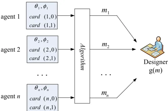
Similar to Ref. [6], in the following we will propose an algorithm that simulates the quantum operations and measurements in Steps 4-7 of the quantum Bayesian mechanism given in Section 4. The amendment here is that now the inputs and outputs are adjusted to the case of Bayesian implementation. The factorγ is also set as its maximum π/2. For nagents, the inputs and outputs of the algorithm are illustrated in Fig. 2. The Matlab program is given in Fig. 3, which is cited from Ref. [6].

Inputs:

1)θi,φi,i=1,· · · ,n: the parameters of agenti’s local operation ˆωi,θi ∈[0, π], φi ∈

[0, π/2].

2) card(i,0),card(i,1), i = 1,_{· · ·} ,n: the information written on the two sides of agenti’s card, wherecard(i,0),card(i,1)_∈Ti× F ×Z+.

Outputs:

mi,i=1,· · · ,n: the agenti’s message that is sent to the designer,mi ∈Ti× F ×Z+.

Procedures of the algorithm:

Step 1: Reading parametersθi andφifrom each agenti∈N (See Fig. 3(a)).

Step 2: Computing the leftmost and rightmost columns of ˆω1⊗ωˆ2⊗ · · · ⊗ωˆn (See

Fig. 3(b)).

Step 3: Computing the vector representation of_|ψ2i= [ ˆω1⊗ · · · ⊗ωˆn] ˆJπ/2|C· · ·CCi.

Step 4: Computing the vector representation of_|ψ3i= Jˆ_π/+₂|ψ2i.

Step 5: Computing the probability distribution_hψ3|ψ3i(See Fig. 3(c)).

Step 6: Randomly choosing a “collapsed” state from the set of all 2n_{possible states}

{|C_{· · ·}CC_i,_{· · ·} ,_|D_{· · ·}DD_i}according to the probability distribution_hψ3|ψ3i.

Step 7: For eachi _∈ N, the algorithm sends card(i,0) (orcard(i,1)) as a message

Fig. 3(d)).

5.3 An algorithmic version of the quantum Bayesian mechanism

In the quantum Bayesian mechanismΓQ_B = (( ˆΣi)i∈N,gˆ), the key parts are quantum

operations and measurements, which are restricted by current experimental tech-nologies. In Section 5.2, these parts are replaced by an algorithm which can be easily run in a computer. Consequently, the quantum Bayesian mechanism ΓQ_B =

(( ˆΣi)i∈N,gˆ) shall be updated to analgorithmic Bayesian mechanismeΓQ_B =((eΣi)i∈N,eg),

which describes a strategy seteΣi ={eσi :Ti 7→[0, π]×[0, π/2]×Ci}for each agent

iand an outcome function_eg: [0, π]n

×[0, π/2]n

×Qi∈NCi → A. A strategy profile

is_eσ = (_eσi,eσ−i), whereeσi = (θi, φi,ci) ∈eΣi, eσ−i : T−i 7→ [0, π]n−1 ×[0, π/2]n−1×

Q

j,_iCj. A Bayesian Nash equilibrium ofeΓ Q

B is a strategy profileeσ∗= (eσ∗1,· · · ,eσ∗n)

such that for any agenti_∈N and for allti ∈Ti,

Ui(eg(eσ∗)|ti)≥ Ui(eg(eσ∗₋i,σe′i)|ti), ∀eσ′i :Ti 7→[0, π]×[0, π/2]×Ci.

As we have shown, the factor γ is set asπ/2 in the algorithmic Bayesian mecha-nism. Thus, the conditionλB_{shall be revised asλ}Bπ/2_.λBπ/2

1 is the same asλB1;λ

Bπ/2 2 :

Consider the payoffto then-th agent, $C···CC >$C···CDcos2(π/l)+$D···DCsin2(π/l).

Working steps of the algorithmic Bayesian mechanismeΓQ_B:

Step 1: Given an SCF f, if f is multi-Bayesian monotonic, goto Step 3.

Step 2: Each agentisetscard(i,0)= (ti, fi,zi), and sendscard(i,0) as the message

mito the designer. Goto Step 5.

Step 3: Each agentisetscard(i,0) = (αi(ti), f,0) andcard(i,1) = (ti, fi,zi) (where

αis specified in the definition of multi-Bayesian monotonic), then submits θi, φi,

card(i,0) andcard(i,1) to the algorithm.

Step 4: The algorithm runs in a computer and outputs messagesm1,· · · ,mn to the

designer.

Step 5: The designer receives the overall message m = (m1,· · · ,mn) and let the

final outcome be g(m) using rules (1)-(3) of the traditional Bayesian mechanism. END.

5.4 Amending sufficient conditions for Bayesian implementation

Proposition 3:Given an SCF f that is incentive compatible and Bayesian mono-tonic:

2) Otherwise f is Bayesian implementable.

Proof: 1) Given an SCF f, since it is multi-Bayesian monotonic, then the mecha-nismeΓQ_B enters Step 3.

Each agentisetsci = (card(i,0),card(i,1)) = ((αi(ti), f,0),(ti, fi,zi)), and submits

θi, φi,card(i,0) andcard(i,1) to the algorithm. Let c = (c1,· · · ,cn). Since

condi-tionλBπ/2 _{is satisfied, then similar to the proof of Proposition 1 in Ref. [6], if then}

agents choose_eσ∗ = (θ∗, φ∗,c), whereθ∗= (0,_{· · ·} ,0

| {z }

n

),φ∗ = (0,_{· · ·} ,0

| {z }

n−l

, π/l,_{· · ·} , π/l | {z }

l

),

then_eσ∗_{∈ B}(eΓQ_B)). In Step 6 of the algorithm, the corresponding “collapsed” state of

nquantum coins is_|C_{· · ·}CC_i. Hence, in Step 7 of the algorithm,mi = card(i,0)=

(αi(ti), f,0) for each agenti∈N. Finally, in Step 5 ofeΓQ_B,eg(eσ∗)=g(m)= f◦α0 f,

i.e., f is not Bayesian implementable.

2) If f is not multi-Bayesian monotonic or condition λBπ/2 _{is not satisfied, then}

the aforementioned _eσ∗ does not exist. Obviously,eΓQ_B is reduced to the traditional Bayesian mechanism. Since the SCF f is incentive compatible and Bayesian mono-tonic, then it is Bayesian implementable.

6 Conclusions

This paper follows the series of papers on quantum mechanism [5,6]. In this paper, the quantum and algorithmic mechanisms in Refs. [5,6] are generalized to Bayesian implementation with incomplete information. It can be seen that for nagents, the time complexity of quantum and algorithmic Bayesian mechanisms areO(n) and

O(2n_{) respectively. Although current experimental technologies restrict the}

quan-tum Bayesian mechanism to be commercially available, for small-scale cases (e.g., less than 20 agents [6]), the algorithmic Bayesian mechanism can help agents ben-efit from quantum Bayesian mechanism immediately.

Acknowledgments

The author is very grateful to Ms. Fang Chen, Hanyue Wu (Apple), Hanxing Wu (Lily) and Hanchen Wu (Cindy) for their great support.

References

[2] T.R. Palfrey and S. Srivastava, On Bayesian implementable allocations.Rev. Econom. Stud.,54(1987) 193-208.

[3] T.R. Palfrey and S. Srivastava, Mechanism design with incomplete information: A solution to the implementation problem.J. Political Economy,97(1989) 668-691.

[4] M.O. Jackson, Bayesian implementation.Econometrica,59(1991) 461-477.

[5] H. Wu, Quantum mechanism helps agents combat “bad” social choice rules. International Journal of Quantum Information, 2010 (accepted).

http://arxiv.org/abs/1002.4294

[6] H. Wu, On amending the sufficient conditions for Nash implementation.Theoretical Computer Science, 2011 (submitted).

http://arxiv.org/abs/1004.5327

[7] R. Serrano, The theory of implementation of social choice rules, SIAM Review 46 (2004) 377-414.

start_time = cputime

% n: the number of agents. For example, suppose there are 3 agents. N={1, 2, 3}. % Suppose the SCF is incentive compatible, Bayesian monotonic and

% multi-Bayesian monotonic. ={1, 2}. n=3;

% gamma: the coefficient of entanglement. Here we simply set gamma to its maximum . gamma=pi/2;

% Defining the array of and . theta=zeros(n,1);

phi=zeros(n,1);

% Reading agent 1’s parameters. For example, theta(1)=0;

phi(1)=pi/2;

% Reading agent 2's parameters. For example, theta(2)=0;

phi(2)=pi/2;

% Reading agent 3’s parameters. For example, theta(3)=0;

phi(3)=0;

π ω

ω = =

π ω

ω = =

ω

ω = =

θ φ =

θ φ =

α

π

% Defining two 2*2 matrices A=zeros(2,2);

B=zeros(2,2);

% In the beginning, A represents the local operation of agent 1. (See Eq (1)) A(1,1)=exp(i*phi(1))*cos(theta(1)/2);

A(1,2)=i*sin(theta(1)/2); A(2,1)=A(1,2);

A(2,2)=exp(-i*phi(1))*cos(theta(1)/2); row_A=2;

% Computing for agent=2 : n

% B varies from to

B(1,1)=exp(i*phi(agent))*cos(theta(agent)/2); B(1,2)=i*sin(theta(agent)/2);

B(2,1)=B(1,2);

B(2,2)=exp(-i*phi(agent))*cos(theta(agent)/2);

% Computing the leftmost and rightmost columns of C= A ⊗ B C=zeros(row_A*2, 2);

for row=1 : row_A

C((row-1)*2+1, 1) = A(row,1) * B(1,1); C((row-1)*2+2, 1) = A(row,1) * B(2,1); C((row-1)*2+1, 2) = A(row,2) * B(1,2); C((row-1)*2+2, 2) = A(row,2) * B(2,2); end

A=C;

row_A = 2 * row_A; end

% Now the matrix A contains the leftmost and rightmost columns of ω

ω ω

ω ⊗ ⊗ ⊗

ω ω

ω ⊗ ⊗ ⊗

ω ω

ω ⊗ ⊗ ⊗

% Computing

psi2=zeros(power(2,n),1); for row=1 : power(2,n)

psi2(row)=A(row,1)*cos(gamma/2)+A(row,2)*i*sin(gamma/2); end

% Computing

psi3=zeros(power(2,n),1); for row=1 : power(2,n)

psi3(row)=cos(gamma/2)*psi2(row) - i*sin(gamma/2)*psi2(power(2,n)-row+1); end

% Computing the probability distribution distribution=psi3.*conj(psi3);

distribution=distribution./sum(distribution);

ψ

ψ ₌ +

ω ω

ω

ψ = ⊗ ⊗ ⊗

ψ ψ

ψ ψ ψ ψ

% Randomly choosing a “collapsed” state according to the probability distribution random_number=rand;

temp=0;

for index=1: power(2,n)

temp = temp + distribution(index); if temp >= random_number

break; end end

% indexstr: a binary representation of the index of the collapsed state % ‘0’ stands for , ‘1’ stands for

indexstr=dec2bin(index-1); sizeofindexstr=size(indexstr);

% Defining an array of messages for all agents message=cell(n,1);

% For each agent , the algorithm generates the message for index=1 : n - sizeofindexstr(2)

message{index,1}=strcat('card(',int2str(index),',0)'); end

for index=1 : sizeofindexstr(2)

if indexstr(index)=='0' % Note: ‘0’ stands for

message{n-sizeofindexstr(2)+index,1}=strcat('card(',int2str(n-sizeofindexstr(2)+index),',0)'); else

message{n-sizeofindexstr(2)+index,1}=strcat('card(',int2str(n-sizeofindexstr(2)+index),',1)'); end

end

% The algorithm sends messages to the designer for index=1:n

disp(message(index)); end

end_time = cputime;

runtime=end_time – start_time

ψ ψ

∈