Munich Personal RePEc Archive
Solving payoff sets of perfect public
equilibria: an example
Du, Chuang
Institute of Economics, Chinese Academy of Social Sciences
7 May 2012
Online at
https://mpra.ub.uni-muenchen.de/38622/
1
Solving Payoff Sets of Perfect Public Equilibria:
An Example
(2011-05-07)
Chuang Du
Abstract
We study an example of infinitely repeated games in which symmetric duopolistic firms
produce experience goods. After consuming the products, short-run consumers only observe imperfect public information about product quality. We characterize perfect public equilibrium
payoff set E(𝛿) of firms for each fixed discount factor δ ∈ [0, 1) when each firm has two action choices, signals follow binomial distributions and the game has a product structure. The set
E(𝛿) turns out a single point or symmetric pentagon for fixed δ. And δ ∈ [0, 1) can be divided into countable infinite subintervals in which E(𝛿) remains constant. The strategies to implement payoffs in boundaries of E(𝛿) are constructed in a recursive way, in which infinite repetition of Nash Equilibrium of stage game could be viewed as an absorbing state in a Markov Process where state transitions are controlled through public signals and optimal punishments in each period.
Keywords: repeated games, imperfect public monitoring, equilibrium payoff sets, duopoly
JEL Classification: C72, C73, D21, D82, L13, L15.
Author Information:
Institute of Economics,
Chinese Academy of Social Sciences,
2
1 Introduction
How to calculate payoff sets of perfect public equilibria for repeated games with long-run and short-run players and with imperfect public monitoring? Existing literature gives only the
upper bound, or limit equilibrium payoff set as discount factor δ → 1, while remains silent on the exact equilibrium payoff sets for fixed δ < 1 when folk theorem fails, and without description on the optimal strategy to implement payoffs on the bound of equilibrium payoff set if signal space is finite (Fudenberg and Levine, 1994; Fudenberg, Levine and Takahashi, 2007). Characterization of the precise form of equilibrium payoff set is valuable not only in theory, but
also in many applications. Because of inevitable existence of multiple equilibria in repeated games, the optimal equilibrium payoff is generally used for prediction in many practical contexts
such as IO. And it is equivalent to solving equilibrium payoff sets in the case of finite signal space since characterize the Pareto boundary is usually equivalent to characterize equilibrium payoff sets1. Moreover, it is more meaningful in real applications to clarify the mechanism through a
detailed description of strategies to achieve boundaries on equilibrium payoff sets.
By a concrete example, we provide an idea to solve payoff sets of perfect public equilibria
for fixed δ in repeated games with long-run and short-run players and with imperfect public monitoring. The idea is not a purely mathematical technique, equilibrium strategies constructed being also of empirical relevance.
Consider the case of two symmetric long-term players each having two hidden action choices in each stage game, and signals of actions follow binomial distributions. For example, in
some duopolistic experience goods2 market, firms may exert low effort or high effort level in the production. It is more likely to produce high quality products when a firm exerts high effort.
However, high effort incurs higher costs. The firm's choice of effort level is hidden action. After consuming the products, consumers observe only product quality, which can be passed to other consumers, e.g., through consumer reports, word of mouth, etc. However, product quality is
unverifiable, i.e., it is difficult to verified by courts and other third-party, thus consumers who buy low-quality products may find themselves difficult to resort to legal claims. Moral hazard problem
naturally occurs. Should consumers believe that a firm choose high effort, the optimal response of the firm would be to choose low effort with lower costs and the expected quality of products would be low then. Rational consumers expect this and would not believe any firm. Thus the
market is full of low quality products and may vanish.
In a market economy, the reputation mechanism can overcome firms’ moral hazard problem. The basic idea is as follows. When firms are long-run players in repeated games, consumers can observe product quality of each firm in last period and make choices in accordance with it. Should the trusted firm deviate to low effort for saving costs in current period, the probability of
losing reputation in next period will increase. If firms are patient enough, such a deviation will be not profitable. Thus patient firms will cherish their reputations and exert high efforts even if
consumers are short-run participants. The reputation mechanism is an example of cooperation in
1
If signals are continuous, then optimal equilibrium payoffs could be implemented by Bang-Bang strategy (Abreu, Pearce and Stacchetti, 1990).
2
3
repeated games with imperfect public monitoring. But how to characterize firms’ equilibrium payoff sets in this repeated games? Note that conventional folk theorem fails here because of the
existence of short-term participants. No matter how patient firms are (even δ → 1), equilibrium payoff set will strictly less than firms’ feasible payoff set (Fudenberg, Kreps and Maskin, 1990).
Consider the following class of equilibria characterized by “states”. Even in repeated games, consumers may not trust any firm, and the result is repetition of static game equilibrium, in which both firms exert low effort, consumers do not buy and the market vanishes. We call this
“state 0 equilibrium”. Consumers may also believe that only one of two firms, firm A, will exert high effort, while the other firm, firm B, is never trusted. If trusted firm A produces low quality products, with a certain probability it will be punished from the next period by consumers.
Punishment here means repetition of static game equilibrium. We call the above situation “state
1 equilibrium”. Consumers might also first trust firm B and try buying. If firm B produce high quality products, consumers will continue to purchase from B; otherwise, with a certain probability all consumers switch from B to A in the next period after low quality of B. Thereafter, if firm A also produce low quality products, all consumers will not trust any firm again. We call
this “state 2 equilibrium”. In addition, consumers may also trust two firms respectively twice, S times and even infinite times. Such as in “state 3 equilibrium”, firm A is trusted twice, while firm B is only trusted one time. In “state ∞ equilibrium”, consumers just switch between the two firms, never out of the market. We call the trusted firm “incumbent firm”, and the other “waiting firm”. Note that due to the uncertainty in production, any firm could not be “incumbent firm” forever.
We find that consumer beliefs described above could be defined and classified in a recursive way, so do accompanying equilibrium mechanisms. For instance, continuation equilibria of state
s equilibrium include state s-1, state s-2 ... state 0 equilibrium. It also can be shown that the lowest discount factor 𝛿𝑠 to ensure existence of state s equilibrium is strictly increasing in s for s ≥ 2. We call all such state s equilibrium “Recursive Belief Equilibrium”, which is a special case of perfect public equilibrium. Under public randomization assumption, the convex hull of payoff set of Recursive Belief Equilibrium constitutes a complete characterization of payoff set of
public perfect equilibrium for any fixed 𝛿. Specifically, for some parameter value of cost function, product function and consumers’ utility function, there exist 0 ≤ 𝛿𝑠 ≤ 1 , 0 ≤ 𝑠 < ∞, 𝛿0= 0 such that for any δ ∈ [ 𝛿𝑠, 𝛿𝑠+1) , state s equilibrium exists, so do state s − 1, s −
2 … 1,0 equilibrium. Define 𝑉̅𝑠as the convex hull of the set of payoff pairs (average discounted expected payoffs) of all possible state s, s − 1, s − 2 … 1,0 equilibrium. We demonstrate that
𝑉̅𝑠 is equal to E(𝛿) , payoff set of perfect public equilibria. Depending on parameter values, it
may be that 𝛿∞ = lim𝑠→∞𝛿𝑠= 1, then δ ∈ [ 𝛿𝑠, 𝛿𝑠+1) , 𝑠 < ∞, 𝛿0= 0 constitute a complete description of δ ∈ [0, 1) ; it may also be that 𝛿∞< 1, then state ∞ equilibrium exists. In the latter case, for any δ ∈ [ 𝛿∞, 1) , 𝑉̅∞is equal to E(𝛿) . In addition, there will still be other parameter values such that only “state 0 equilibrium” exists for any δ ∈ [0, 1) . Thus payoff set of public perfect equilibrium is trivially equal to a single point, “state 0 equilibrium” payoff. Note that due to symmetry of the game, any state s equilibrium payoffs include two symmetric points: Let (𝑣𝑖𝑠, 𝑣𝑗𝑠) is state s equilibrium payoff pairs, so is (𝑣𝑗𝑠, 𝑣𝑖𝑠) , where the first component in brackets represents firm i's payoff and second component firm j (j ≠ i). It can also be shown that, for any δ < 1 , if 𝑣𝑠 is the largest payoff of incumbent firm in all possible state
4
𝑤𝑠 > 0 is the payoff of “waiting firm” in state s equilibrium when incumbent’s payoff is v .
The intuition is as follows. The game analyzed in this paper has the product structure,
namely, the hidden action of each long-run player has a public signal and the signals are independent of each other. Each signal is a sufficient statistic of the player’s hidden action, thus for all equilibrium payoff pairs, strategies to implement them could be equivalently expressed as
if each firm's continuation payoffs rely solely on its own signal (Holmstrom, 1982). The range to search for the optimal equilibrium strategy is then greatly reduced. For instance, performance
comparison evaluation is unnecessary. In recursive belief equilibrium, continuation payoffs of the incumbent firm depend only on its own signal. Although continuation payoffs of the waiting firm depend on the signal of the incumbent, the waiting firm is just waiting, no incentive problem
accompanied. In addition, although there are only two firms, two actions, binomial distribution of signals in the example, it could easily be extended to N firms, N actions and any type of signal
distribution, as long as firms are symmetric and the game has product structure.
The idea in this article is similar to Upwind Gauss-Seidel method in numerical computation of dynamic programming problem. The state transition between the incumbent and waiting firm
from state s to s − 1 may be regarded as a Markov Process, where state transition probabilities are endogenous, depending on probabilities of consumers’ punishments after the incumbent firm producing low-quality products. And state 0 is the only absorbing state, the equilibrium payoffs of which is easy to calculate, equaling to infinitely repetitions of static game Nash equilibrium. State 1 equilibrium payoffs could be calculated according to state 0 equilibrium,
while state 2 equilibrium payoffs could be calculated according to state 1 equilibrium, and so on. The following words in Judd (1998) provide a good description of the idea. (See also Figure 1)
"We see here that if the state flows in the directions of the solid arrows, the proper direction for us to construct the value function is in the opposite," upwind ", direction. Another way to
express this is that information naturally flows in the upwind direction. For example, information about state 1 tells us much about states 2 ..., but we can evaluate state 1 without knowing
anything about states 2 ... Again, a single pass through the states will determine the value of the indicated policy ... In general, once we ascertain the value of the problem at the stable steady states, we can determine the value at the remaining states. "
---- Judd (1998, pp.420-421)
(Insert Figure 1 Here)
In addition, the dynamics of reputations on oligopolistic markets are revealed in this paper
in a pure moral hazard context, which may be an interesting complement to reputation models introducing private information of firms, such as Kreps and Wilson (1982), Milgrom and Roberts
(1982). While they concentrate on how reputation is built step by step, firms lose reputation one-off in their models. On the contrary, we concentrate on how reputation vanishes step by step. For instance, the optimal probability of punishment in equilibrium (the probability of losing
consumers when the incumbent firm producing low-quality products) will becomes lower and lower as chances to be incumbent again reduces. Consumers are more and more "tolerant", or
5
Samuelson, 2004), but because firms have less and less opportunities to be incumbent again, which itself constitutes a growing potential punishment. For the same reason, the critical
discount factor to support state s equilibrium is increasing in s for s ≥ 2 . We quoted some empirical literature in part 6 of this article to verify the relevance of reputation dynamics.
The rest of the paper is structured as follows. In Section 2 we discuss related literature.
Section 3 spells out the model setup. In Section 4 we characterize recursive belief equilibrium (state s equilibrium) payoff set and in Section 5 we prove that the set constitutes a complete characterization of perfect public equilibrium payoff set in the model. Relevant studies are cited in Section 6 to verify the empirical relevance of recursive belief equilibrium. Section 7 contains the conclusions and further questions.
2 Related Literature
Our paper is closely related to the literature on computation of payoff set of perfect public equilibrium. Abreu, Pearce and Stacchetti (1990) first present a general algorithm of set iteration, similar to value function iteration in dynamic programming with a single decision-maker. However,
set iteration is generally not tractable in specific operations. The direct application of set iteration algorithm for solving equilibrium payoff set is now mainly in the framework of repeated games
with perfect monitoring, and can only obtain upper and lower bounds of equilibrium payoff set through numerical computation (Judd, et al, 2003) 3. Abreu and Sannikov (2011) provide a new algorithm to calculate pure strategy SPE in 2-person repeated games with perfect monitoring and
with public randomization. For repeated games with imperfect public monitoring, Fudenberg, Levine and Maskin (1994), Fudenberg and Levine (1994) give explicit methods to calculate
equilibrium payoff set (upper bound) under limited signal space. Fudenberg and Levine (1994) presents a general algorithm for computing the upper bound of set of payoffs of perfect public
equilibria of repeated games with long-run and short-run players; and shows that the upper bound is equal to limit equilibrium payoff set as δ → 1 if the game meets some condition of full rank. Fudenberg, Levine and Takahashi (2007) further solve the limit set of perfect public
equilibrium payoff when full rank condition fails. Horner, Sugaya, Takahashi, and Vieille (2011) extends Fudenberg and Levine (1994)’s algorithm to general stochastic games. Horner, Takahashi and Vieille (2012) further provides a dual characterization of the limit set of perfect public equilibrium payoffs in stochastic games and shows that, in the context of repeated games, this limit set of payoffs is a polytope when attention is restricted to equilibria in pure strategies.
A second strand of relevant literature is that on reputation mechanisms of experience goods markets. There are a lot of studies on reputation mechanisms in different market structure, such
as Klein and Leffler (1981), Shapiro (1983), Horner (2002), Rob and Fishman(2005), Rob and Sekiguchi (2006), Cai and Obara (2009). In this strand, our paper is perhaps most closely related to Rob and Sekiguchi (2006), which studies "turnover equilibrium" in a duopoly market, similar to
state ∞ equilibrium in our paper. In addition, Rob and Fishman (2005) also shows the dynamics of reputation in a pure moral hazard framework, but it is in the context of monopolistic
competition market with infinite number of firms. And the concern of Rob and Fishman (2005) is the gradual accumulation of reputation, while firms lose reputation one-off. The focus of
3
6
reputation dynamics in our article is how reputation vanishes gradually.
3 The Model
There are two long-lived firms in the market. Time is discrete and the horizon is infinite. In each period, each firm and consumers play the following stage game. The consumers decide
whether to purchase one unit of the firm’s products. If they do not buy from the firm, both the
consumers and the firm get a payoff of zero. If they decide to buy from the firm, their payoffs
decide on the firm’s product quality. The firm decides whether to exert high effort 𝑎ℎ(or, provide high quality) or exert low effort 𝑎𝑙(or, provide low quality). The firm incurs an effort cost /quality cost of c for providing high effort/quality, 0 for providing low effort/quality, where c > 0 .
The consumers’ expected benefit is u if the firm choose 𝑎ℎ, and is 0 if the firm choose 𝑎𝑙,
where u > 0. Market price is fixed at p = u 4. The stage game is depicted below in the normal form.
Firm
Low High
Consumers Not Buy 0, 0 0, 0
Buy −u, u 0, u − c
We assume u − c > 0, hence high effort/quality is more efficient than no trade. However,
Should consumers choose “Buy”, the optimal response of the firm would be “Low” (effort/quality). Thus the unique equilibrium outcome is (Not Buy, Low), resulting in payoffs (0, 0).
We suppose that in each period there are identical consumers with measure 1, who
purchase the products only once. So consumers will maximize their current period payoffs. If consumers are indifferent between “Buy” and “Not Buy”, they will choose “Buy”.
If the firm’s effort in each period were publicly observable, it would be straightforward to
show that the efficient outcome (Buy, High) can be supported when firms are patient enough. Let
δ be the firms’ common discount factor. It can be easily checked that the efficient outcome is
attainable in every period if and only if δ ≥ c/u.
We consider an environment in which a firm’s effort is not public information, but rather its noisy public signal 𝑦𝑖 ∈ {𝑦ℎ, 𝑦𝑙}, 𝑖 = 1,2 becomes available at the end of each period. For each firm i, the probability of 𝑦 = 𝑦ℎis μh and 𝑦 = 𝑦𝑙is 1 − μh if firm i exerts high effort; the
4
7
probability of 𝑦 = 𝑦ℎis μl and 𝑦 = 𝑦𝑙is 1 − μl if firm i exerts low effort, where μh> μl> 0. Signals of different firm, 𝑦1 and 𝑦2, are independent. We can interpret public signals 𝑦𝑖as quality level of firm i’s products and there are uncertainties in production processes. Or we can interpret 𝑦𝑖as some subjective signals on quality because communications between current period consumers and future consumers are imperfect.
Following Fudenberg and Levine (1994), a rigorous description of the repeated games is as follows. Let number 1, 2 represent two long-run players, firms and SR represents short-run
players, consumers. In each stage game, each player i = 1,2, SR simultaneously chooses a (pure) action aifrom a finite set 𝐴𝑖 . Ai= {ah, al} for i = 1,2, where ah represents High Effort,
alrepresents Low Effort. Ai= {Buy, Not Buy} for i = SR . Note that aSR= {aSR,1, aSR,2} is a
vector where aSR,i represents consumers action on firm i ( i = 1,2). Each action profile
a = (a1, a2, aSR) induces a probability distribution over public signals y = (y1, y2) , 𝑦𝑖∈ {𝑦ℎ, 𝑦𝑙, 𝑦𝑛𝑢𝑙𝑙}, i = 1,2, where 𝑦ℎ represents high quality, 𝑦𝑙 represents low quality and 𝑦𝑛𝑢𝑙𝑙 represents no trade. For a given action profile a, let πy(a) denote the probability
of y and πi(𝑎), i = 1,2 denote the marginal probability for the public signals. Obviously in our model we have πy(a1, a2, aSR) = π1(a1, αSR,1)π2(a2, aSR,2) , π1(a1, aSR,1) = π2(a1, aSR,1). And for i = 1,2
πi(aH, Not Buy) = πi(aL, Not Buy) = (0,0,1) πi(aH, Buy) = (𝜇ℎ, 1 − 𝜇ℎ, 0)
πi(aL, Buy) = (𝜇𝑙, 1 − 𝜇𝑙, 0)
To each action profile a,player i’s expected payoff ( 𝑖 = 1,2 ) is gi(a) = ∑y∈Yπy(a)ri(y), where ri(y) is player i’s payoff ( 𝑖 = 1,2 ) for signal y .
Let αibe mixed actions for each player i. For each profile α = (αi, αj, αSR) of mixed actions, we can compute the induced distribution over public signals, πy(α) = ∑a∈Aπy(a)α(a); and the expected payoffs, gi(α) = ∑y∈Y∑a∈Aπy(a)α(a)ri(y) . Denote the profile where player i plays αiand all other players follow profile α by (αi, α−i). πy(αi, α−i) and gi(αi, α−i) are defined in the similar way.
The objective of each long-run player i = 1,2 is to maximize the average discounted value of per-period payoffs using the common discount factor δ . If {gi(t)} is a sequence of payoffs for long-run player i , player i’s average discounted expected payoff will be: (1 − δ) ∑∞t=1δt−1gi(t) . In the repeated game, in each period t = 1,2, …, the stage game is played, and the corresponding public outcome is then revealed. The public history at the end of period t is h(t) = {y1, y2, … , yt} . We also let h(0) denote the null public history in which nothing has happened. A public strategy for long-run player i ( i = 1,2) is a sequence of maps mapping public history to mixed actions. A public strategy for the period- t consumers is a map from the public information h(t − 1) to mixed actions. We define E(δ) ⊂ ℝ2to be the set of average present values for the long-run player that can arise in perfect public equilibria when the discount factor
8
4 Recursive Belief Equilibrium
Define "recursive beliefs” as follows.
Definition 1: A recursive belief 𝐬 (𝟎 ≤ 𝐬 ≤ ∞) includes the following state 𝐬 to state 0. (i) state 𝐬 (𝒔 ≥ 𝟐) : all consumers believe that only one firm, say firm 1, exert high effort. If the public signal of firm 1 is 𝒚𝒉at the end of current period, consumers’ beliefs will remain unchanged in next period; if the public signal of firm 1 is 𝒚𝒍at the end of current period, next period consumers’ beliefs will transit into state s-1 with probability 𝛒𝐬 (𝟎 < 𝛒𝐬≤ 𝟏) and remain in state s with probability 𝟏 − 𝛒𝐬. Call the trusted firm “incumbent firm” in state 𝐬 , the
other firm “waiting firm” in state 𝐬. Let 𝐯𝐬, 𝐰𝐬be (per period) average discounted expected payoffs of “incumbent firm” and “waiting firm” from state 𝐬 to state 0, respectively.
(ii) state s-1: all consumers believe that only the “waiting firm” in state 𝐬, firm2, will high effort. If the public signal of firm 2 is 𝒚𝒉at the end of current period, consumers’ beliefs will remain unchanged in next period; if the public signal of firm 2 is 𝒚𝒍at the end of current
period, next period consumers’ beliefs will transit into state s-2 with probability 𝛒𝐬−𝟏 (𝟎 <
𝛒𝐬−𝟏 ≤ 𝟏) and remain in state s with probability 𝟏 − 𝛒𝐬−𝟏. Again, call the trusted firm, firm 2,
“incumbent firm” in state 𝐬 − 𝟏; the other firm, firm 1, “waiting firm” in state 𝐬 − 𝟏. Let
𝐯𝐬−𝟏, 𝐰𝐬−𝟏be average discounted expected payoffs of “incumbent firm” and “waiting firm”
from state 𝐬 − 𝟏 to state 0, respectively.
(iii) state 0: all firms are not to be trusted. Payoff pair of two firms is (𝐯𝟎, 𝐰𝟎) = (𝟎, 𝟎).
The above definition means that consumers trust the same one of two firms in state s, s-2, ... and trust the other firm in state s-1 s-3, ... And v1, v2, v3, … denote the average payoff of incumbent firm from state 1, 2, 3, ... to state 0 respectively, while w1, w2, w3, … denote the average payoff of waiting firm from state 1, 2, 3, ...to state 0 respectively. To facilitate the
presentation, we call a perfect public equilibrium with recursive beliefs as “recursive belief equilibrium”. The formal definition is as follows.
Definition 2: A recursive belief equilibrium is a perfect public equilibrium where
consumers and firms take the following strategies: (i) the consumers' strategies are in line with recursive beliefs; (ii) each firm exerts high effort if it is a “incumbent firm”, and exerts low effort if it is a "waiting firm” or if it is in state 0.
We also call a recursive belief equilibrium “state s equilibrium” if the consumers' initial belief is at state s. The critical discount factor of stats s equilibrium, the minimum discount factor to support state s equilibrium, is denoted by δs. According to the definition of recursive belief, it is obviously that if state s equilibrium exists, state s' equilibrium exists for any s′< 𝑠. Thus the critical discount factor δs is non-decreasing in s.
Obviously, “state 0 equilibrium” always exists for any discount factor. It is just infinite repetition of static game Nash equilibrium.
In any state s (s ≥ 1), it is clearly rational for consumers taking recursive beliefs given
9
the consumers’ and waiting firm's strategy? Here we look at the trade-off faced by the incumbent. According to Abreu, Pearce and Stacchetti (1990), the average discounted payoff of the
incumbent, vs , can be decomposed into a weighted sum of current period payoff and continuation payoffs from next period, weighted by discount factor:
𝑣𝑠 = (1 − 𝛿)(𝑢 − 𝑐) + 𝛿{[1 − (1 − μh)ρs]𝑣𝑠 + (1 − μh)ρs𝑤𝑠−1} (1)
The first term on the right of (1) is the current period payoff of the incumbent firm when exerts high-effort, the second item is expected continuation payoffs from next period when exerts high
effort, discounted to current period. (1 − μh)ρsis the probability to be punished in next period when the incumbent firm exerts high effort, i.e., the transition probability from state s to state s-1. [1 − (1 − μh)ρs] is the probability of remaining in state s when the incumbent exerts high effort. Note that the incumbent firm in state s is just the waiting firm in state s-1.
Accordingly, to make optimal the incumbent choosing high effort, the following incentive
compatibility conditions is necessary:
𝑣𝑠 ≥ (1 − 𝛿)𝑢 + 𝛿{[1 − (1 − μl)ρs]𝑣𝑠 + (1 − μl)ρs𝑤𝑠−1} (2) Should the incumbent deviate to low effort, the cost savings in current period is c, but in the next
period the transition probability from state s to state s-1 would increase from
(1 − μh)ρsto (1 − μl)ρs. Inequality (2) means that such a deviation is not profitable. It is easy to
prove that the incumbent's payoff is maximized when (IC) condition binds.
In addition, in state s the waiting firm has no incentive problem and is just waiting passively: waiting for the failure of the incumbent. The waiting firm’s average payoff is:
𝑤𝑠 = 𝛿{[1 − (1 − μh)ρs]𝑤𝑠 + (1 − μh)ρs𝑣𝑠−1} (3) According to (1), (2) and (3), there are multiple equilibria for state s since incentive compatibility condition need not bind. The following Proposition 3 gives closed solutions
to vs , ws and optimal probability of punishment ρs when the incumbent firm’s payoff is maximized, (IC) binds, in all possible state s equilibria.
Proposition 3: If state 𝐬 (𝒔 ≥ 𝟏) equilibrium exists,the following results hold when the
incumbent firm’s equilibrium payoff is maximized,
𝐯𝐬(𝜹) = 𝐯 ≡ 𝐮 − 𝐜 −(𝟏 − 𝛍(𝛍 𝐡)𝐜
𝐡− 𝛍𝐥)
𝛒𝐬(𝜹) = {
𝛈(𝜹)[𝟏 − (𝟏 − 𝛍𝐡 𝐫 )
𝐬−𝟏
], 𝐢𝐟 𝐬 ≥ 𝟐 𝐚𝐧𝐝 𝐫 ≠ 𝟏 − 𝛍𝐡
(𝑠 − 1)(1 − δ)
δr , if s ≥ 2 and r = 1 − μh (𝟏 − 𝛅)
𝛅𝐫 , 𝐢𝐟 𝐬 = 𝟏
𝐰𝐬(𝜹) = 𝒘𝒔∗ ≡
{
(𝟏 − 𝛍𝐡) [𝟏 − (𝟏 − 𝛍𝐫 )𝐡 𝐬−𝟏
] 𝐯 [𝐫 − (𝟏 − 𝛍𝐡)] + (𝟏 − 𝛍𝐡) [𝟏 − (𝟏 − 𝛍𝐫 )𝐡
𝐬−𝟏 ]
, 𝐢𝐟 𝐬 ≥ 𝟐, 𝐫 ≠ 𝟏 − 𝛍𝐡 (1 − μh)(𝑠 − 1)v
𝑟 + (1 − μh)(𝑠 − 1) , if 𝐬 ≥ 𝟐, r = 1 − μh (𝟏 − 𝛍𝐡)𝐯
10
where 𝐫 ≡𝐯(𝛍𝐡−𝛍𝐥)
𝐜 , 𝛈(𝜹) ≡ { (𝟏−𝛅)
𝛅 ∙ 𝟏 [𝐫−(𝟏−𝛍𝐡)]} . Proof:
Combine (1) and (2), we have
(1 − δ)𝑐
δ ≤ (μh− μl)ρs(vs− ws−1) (4)
It is equivalent to
ws−1≤ vs−δ(μ(1 − δ)𝑐
h− μl)ρs
Substitute above inequality for ws−1 in equation (1), we can obtain
vs≤ (1 − δ)(𝑢 − c) + δ {[1 − (1 − μh)ρs]vs+ (1 − μh)ρs[vs−δ(μ(1 − δ)c h− μl)ρs]}
Rearrange it,
vs≤ 𝑢 − c −(1 − μ(μ h)𝑐
h− μl)
Obviously vsis maximized when IC condition binds,
vs= 𝑢 − c −(1 − μ(μ h)𝑐
h− μl) ≡ v (s ≥ 1) ws−1= [𝑢 − c −(1 − μ(μ h)𝑐
h− μl)] −
(1 − δ)𝑐
δ(μh− μl)ρs (5)
And by (3), we have
ws=[1 − δ + δ(1 − μδ(1 − μh)ρs∙ v
h)ρs]
Or equivalently, for s ≥ 2
ws−1=1 − δ + δ(1 − μδ(1 − μh)ρs−1∙ v
h)ρs−1 (6)
Combine (5) and (6) ,
δ(1 − μh)ρs−1∙ v
1 − δ + δ(1 − μh)ρs−1= v −
(1 − δ)𝑐 δ(μh− μl)ρs
Thus,
ρs=v(μ 1
h− μl)/c ∙ [(1 − μh)ρs−1+ 1 − δ
δ ] ≡ 1
r ∙ [(1 − μh)ρs−1+ 1 − δ
δ ] (7)
Moreover, when (IC) condition binds, (4) becomes
(1 − δ)𝑐
δ = (μh− μl) ρs(vs− ws−1) (8)
By initial conditions v1= v, w0= 0 and (8), we have
𝜌1∗=δ(μ(1 − δ)𝑐 h− μl)v ≡
(1 − δ) δ𝑟
When s = 2 , v2= v, w1= 0 , by (8) we obtain
11 And from (3) we have
𝑤2∗= δ(1 − μh)𝜌2 ∗∙ v [1 − δ + δ(1 − μh)𝜌2∗] =
(1 − μh)v 𝑟 + (1 − μh)
When s = 3 , v3= v, w2= 𝑤2∗, by (8) we obtain
𝜌3∗=δ(μ (1 − δ)𝑐
h− μl)(v − 𝑤2∗) = { (1 − δ)
δ ∙
1
[r − (1 − μh)]} {1 − [
(1 − μh) 𝑟 ]
2 } 𝑤3∗ = δ(1 − μh)𝜌3
∗∙ v [1 − δ + δ(1 − μh)𝜌3∗] =
(1 − μh)[𝑟 + (1 − μh)]v r2+ (1 − μh)[𝑟 + (1 − μh)]
When s = 4 , v4= v, w3= 𝑤3∗, by (8) we obtain
𝜌4∗ =δ(μ (1 − δ)𝑐
h− μl)(v − 𝑤3∗) =
(1 − δ) δ
[r2+ (1 − μ
h)[𝑟 + (1 − μh)]] r3
= {(1 − δ)δ ∙[r − (1 − μ1
h)]} {1 − [
(1 − μh) 𝑟 ]
3
}
Solving difference equation on ρs, (7), with initial condition 𝜌2∗ =(1−δ)
δ𝑟 , we obtain, for s ≥ 2 ρs= 𝜌𝑠∗≡
{
η(𝛿)[1 − (1 − μh r )
s−1
], if r ≠ 1 − μh
(𝑠 − 1)(1 − δ)
δr , if r = 1 − μh
Where r ≡v(μh−μl)
c , η(𝛿) ≡ { (1−δ)
δ ∙ 1 [r−(1−μh)]} .
Therefore, for s ≥ 2
ws=[1 − δ + δ(1 − μδ(1 − μh)ρs∙ v
h)ρs]
= {
(1 − μh) [1 − (1 − μr )h s−1
] v [r − (1 − μh)] + (1 − μh) [1 − (1 − μr )h
s−1 ]
, if r ≠ 1 − μh (1 − μh)(𝑠 − 1)v
𝑟 + (1 − μh)(𝑠 − 1) , if r = 1 − μh
Q.E.D
By Proposition 3, the maximal payoff that the incumbent firm can obtain in any recursive
belief equilibrium is less than the maximal feasible payoff (v < 𝑢 − 𝑐) even δ → 1. Folk Theorem fails here because there are short-run players and uncertainty in production process, punishment
is eventually unavoidable to maintain firm’s incentive to exert high effort although consumers
know that on the equilibrium path bad signal comes only from bad luck. And 𝑤𝑠∗ is a weighted sum of v and 0, where the weight depends on belief state 𝑠 .
12
expected payoff will be negative when the incumbent firm exerts low effort with positive
probability in the equilibrium path, “Buy” will not be an optimal response then.
Note that r ≡v(μh−μl)
c , so “r = 1 − μh " is equivalent to "u − c =
2(1−μh)c
(μh−μl) ". For s ≥ 2, let
δs≡
{ 1
1 + r , if 𝑠 = 1 1
1 + [r − (1 − μh)] [1 − (1 − μh
r ) s−1
]
, if s ≥ 2 and u − c ≠2(1 − μ(μ h)c h− μl) 𝑠 − 1
r + s − 1 , if s ≥ 2 and u − c =
2(1 − μh)c (μh− μl)
Proposition 4: Necessary and sufficient conditions for the existence of state 𝐬 equilibria. (i) State 𝐬 (𝟏 ≤ 𝐬 < ∞ ) equilibrium exists if and only if 𝐮 − 𝐜 >(𝟏−𝛍𝐡)𝐜
(𝛍𝐡−𝛍𝐥) and 𝛅 ≥ 𝜹𝒔. (ii) State ∞ equilibrium exists if and only if 𝐮 − 𝐜 >𝟐(𝟏−𝛍𝐡)𝐜
(𝛍𝐡−𝛍𝐥) and 𝛅 ≥
𝟏 r+μh . (iii) Only state 𝟎 equilibrium exists if 𝐮 − 𝐜 <(𝟏−𝛍𝐡)𝐜
(𝛍𝐡−𝛍𝐥) or 𝛅 < 𝜹𝟏.
Proof:
By the proof of Proposition 3, a necessary condition for the existence of state s equilibrium is:
v ≡ 𝑢 − c −(1 − μ(μ h)𝑐 h− μl) > 0
It is equivalent to u >(1−μl)c
(μh−μl) .
Moreover, when s = 1, the minimum δ satisfying inequality (4) could be obtained by letting
ρ1= 1 and (4) binds. Thus the critical discount factor for state 1 equilibrium is: 𝛿1= 1
1 + v(μh− μl) 𝑐
≡1 + r1
When s ≥ 2 , the existence of state s equilibrium requires ρs≤ 1. Hence for r ≠ 1 − μh, or equivalently for u − c ≠2(1−μh)c
(μh−μl) ,
{(1 − δ)δ ∙[r − (1 − μ1
h)]} [1 − ( 1 − μh
r ) s−1
] ≤ 1 ⇔ δ ≥ 1
1 + [r − (1 − μh)] [1 − (1 − μh
r ) s−1
]
= 𝛿𝑠
Hence, 𝛿∞ = 1
13
2(1−μh)c
(μh−μl) . 𝛿∞= lim𝑠→∞𝛿𝑠= 1 and state ∞ equilibrium does not exist for δ < 1 if r < 1 − μh.
For r = 1 − μhor equivalently u − c =2(1−μh)c
(μh−μl) ,
𝜌𝑠∗=(𝑠−1)(1−δ)δr ≤ 1, ⇔ δ ≥r + s − 1 = 𝛿𝑠 − 1 𝑠
Moreover, 𝛿∞ = lim𝑠→∞𝛿𝑠 = 1 and state ∞ equilibrium does not exist for δ < 1 if r = 1 − μh. The conclusions hold by the definition of δs.
Q.E.D
By Proposition 3 and 4, the critical discount factor 𝛿1= 𝛿2 , optimal probability of punishment 𝜌2∗= 𝜌1∗ . Because in “state 2 equilibrium”, the incumbent firm will become a waiting firm in “state 1 equilibrium” and its continuation payoff will be 0 after punished in state 2; while in state 1 equilibrium, the incumbent firm will never be trusted and its continuation payoff
will also be 0 after punished in state 1. The incentives faced by them are the same, so are optimal punishment probabilities and the critical discount factors. However, 𝛿4≠ 𝛿3, 𝜌4∗≠ 𝜌3∗. The incumbent firm in state 4 equilibrium has another chance, to be incumbent in state 2, and the
incumbent firm in state 3 equilibrium has also another chance, to be incumbent in state 1; but continuation payoffs of the two after being punished are different, hence different for optimal
probabilities of punishment and critical discount factors. In state 4 equilibrium the incumbent
firm’s continuation payoff after being punished, 𝑤3∗, depends on the waiting time in state 3,
which in turn depends on the optimal probability of punishment on the incumbent firm in state 3;
while in state 3 equilibrium the incumbent firm’s continuation payoff after being punished, 𝑤2∗,
depends on the waiting time in state 2, which in turn depends on the optimal probability of
punishment on the incumbent firm in state 2. Nevertheless, the optimal probability of punishment on the incumbent firm in state 3 is different from that of state 2, for the incumbent
firm in state 3 will have another chance, to be incumbent in state 1, while the incumbent in state 2 will be no chance after being punished.
More generally, by Proposition 3 and 4, we have the following corollary.
Corollary 5: For all 𝐬 ≥ 𝟐 ,
(i) The critical discount factor 𝜹𝒔is strictly increasing in s.
(ii) The optimal probability of punishment 𝝆𝒔∗ is strictly increasing in s. (iii) The equilibrium payoff of the waiting firm 𝒘𝒔∗ is strictly increasing in s..
Proof:
(i) If s ≥ 2 and r > 1 − 𝜇ℎ , 𝑟−(1−μh)
1−(1−μhr )s−1 will be strictly decreasing in s,
hence by definition of 𝛿𝑠 , 𝛿𝑠 will be strictly increasing in s. If s ≥ 2 and r < 1 − 𝜇ℎ ,
𝑟−(1−μh)
14
1 − μh , δs=r+s−1𝑠−1 will obviously be strictly increasing in s.
(ii) If s ≥ 2 and r = 1 − μh , 𝜌𝑠∗ =(𝑠−1)(1−δ)
δr will obviously be strictly increasing in s.
If s ≥ 2 and r ≠ 1 − μh,
d𝜌𝑠∗
ds = −η(𝛿) ( 1 − μh
r ) s−1
ln (1 − μr )h
Thus when 1 − μh> 𝑟 , η(𝛿) ≡ {(1−δ)
δ ∙ 1
[r−(1−μh)]} < 0 , ln (
1−μh
r ) > 0 , d𝜌𝑠∗
ds > 0 ; when 1 − μh< 𝑟 , η > 0 ,ln (1−μrh) < 0 ,d𝜌𝑠
∗
ds > 0 .
(iii) If s ≥ 2 and r = 1 − μh, 𝑤𝑠∗ = (1−μh)(s−1)v
r+(1−μh)(s−1)will obviously be strictly increasing in s.
If s ≥ 2 and r ≠ 1 − μh,
𝑤𝑠∗ =
(1 − μh) [1 − (1 − μr )h s−1
] v [r − (1 − μh)] + (1 − μh) [1 − (1 − μr )h
s−1 ] = [r − (1 − μv
h)] (1 − μh) [1 − (1 − μr )h
s−1 ]+ 1
As in (i), [r−(1−μh)]
[1−(1−μhr )s−1] is strictly decreasing in s, hence 𝑤𝑠
∗is strictly increasing in s.
Q.E.D
Corollary 5 reveals interesting dynamics on firm’s reputation. When we consider the timing of the game in reality, then for any state s equilibrium, it must be first to experience the state s, then the state s-1, s-2... 1, 0 in turn. So the optimal probability of punishment will decrease in the
process of equilibrium state. Consumers are more and more "tolerant", or less and less sensitive
to incumbent firm’s quality signal as from state s to s-1…2, 1. It is not any kind of "inertia" of
consumers’ belief due to long-term success of firm (such as in Crips, Mailath and Samuelson, 2004), but because firms have less and less opportunities to be incumbent again, which itself constitutes a growing potential punishment. For the same reason, the critical discount factor to
support state s equilibrium is strictly decreasing in the process of equilibrium state.
15
5 Perfect Public Equilibrium Payoff Set
Consider a Euclidean Plane, where horizontal coordinate represents firm 1’s payoff, vertical
coordinate represents firm 2’s payoff. Since consumers are short-run players and maximize
current period payoff, the joint payoff of two firms in each period cannot be more than u − c. The feasible payoff set of two firms is therefore a triangle in this plane: {(v1, v2): 0 ≤ v1≤ u − c,
0 ≤ v2≤ u − c, 0 ≤ v1+ v2≤ u − c} .
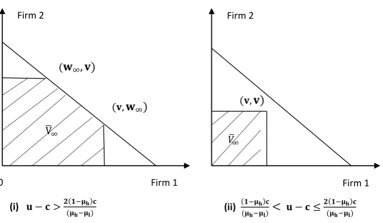
Define V̅s as the pentagon connected by following vertices:
(0,0), (v, 0), (0, v), (v, 𝑤𝑠∗), (𝑤𝑠∗, v) , where (v, 𝑤𝑠∗), (𝑤𝑠∗, v) are payoff profiles for states
equilibrium when the incumbent firm’s payoff is maximized and firm 1 or 2 is the incumbent firm
respectively; (v, 0), (0, v) are payoff profiles for state 1 equilibrium when firm 1 or 2 is the incumbent firm respectively and (0,0) is payoff profile for state 0 equilibrium. Note that points at the connected lines and inner regions could be supported as equilibrium payoffs through a
public randomization on above five points.
𝑉̅𝑠 degenerates to a single point (0,0) when s = 0 . And when s = 1, V̅s degenerates to a
triangle since 𝑤1∗ = 0 . However, by proposition 3 and 4, state 2 equilibrium exists whenever state 1 equilibrium exists. Thus we omit V̅1
By proposition 3 and 4, 𝑉̅𝑠 are as following Figure 2 (shaded region) when state s → ∞.
v∞+ w∞= μh− c if v >(1−μ(μh−μh)𝑐l) , so the boundary of feasible payoff set is reached.
Otherwise, v ≤(1−μh)𝑐
(μh−μl), lim𝑠→∞𝑤𝑠
∗= v , v + lim
𝑠→∞𝑤𝑠∗= 2v < μh− c , thus the boundary of
feasible payoff set may not be supported as recursive belief equilibrium.
(Insert Figure 2 here)
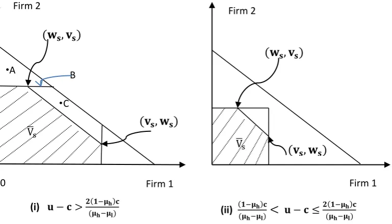
More generally, for 2 ≤ s < ∞ , V̅sare as following Figure 3. (Insert Figure 3 here)
Our purpose is to prove that, V̅s= 𝐸(𝛿) for any δ and 0 ≤ s ≤ ∞, where 𝐸(𝛿) is the payoff set of perfect public equilibria of the game given δ . Thus any point similar to A in Figure 3 could not be an PPE payoff profile, and any point similar to B, C in Figure 3 would not be PPE
payoff profiles if they could not be supported by recursive equilibrium payoff profiles. We first prove an important lemma before providing the critical proposition and its proof.
Lemma 6: for any { 𝒗𝟏, 𝒗𝟐} ∈ 𝑬(𝜹) , there exist { 𝒘𝟏(𝒚𝟏), 𝒘𝟐(𝒚𝟐)} ∈ 𝑬(𝜹) and 𝐚 ∈ 𝐀 such that, (𝐢, 𝐣 = 𝟏, 𝟐)
𝒗𝒊= (𝟏 − 𝜹)𝒈𝒊(𝒂𝒊, 𝜶−𝒊) + 𝜹 ∑ 𝝅𝒊(𝒂𝒊, 𝜶𝑺𝑹,𝒊)𝒘𝒊(𝒚𝒊) 𝒚𝒊∈{𝑦ℎ,𝑦𝑙,𝑦𝑛𝑢𝑙𝑙}
16
And if 𝒂𝒊= 𝒂𝒉 , 𝒂𝒋= 𝒂𝒍, there will be 𝒗𝒋= 𝜹 ∑ 𝝅𝒚𝒊 𝒊(𝒂𝒊, 𝜶𝑺𝑹,𝒊)𝒘𝒋(𝒚𝒊) . Proof:
According to APS (1990), for any { 𝑣1, 𝑣2} ∈ 𝐸(𝛿) , there exist { 𝑤𝑖(𝑦𝑖, 𝑦𝑗), 𝑤𝑗(𝑦𝑖, 𝑦𝑗)} ∈
𝐸(𝛿) and a ∈ A such that
𝑣𝑖 = (1 − 𝛿)𝑔𝑖(𝑎𝑖, 𝛼−𝑖) + 𝛿 ∑ 𝜋𝑦(𝑎𝑖, 𝑎𝑗, 𝛼𝑆𝑅)𝑤𝑖(𝑦𝑖, 𝑦𝑗) 𝑦
𝑓𝑜𝑟 𝑎𝑛𝑦 𝑎𝑖 𝑠. 𝑡. 𝛼𝑖(𝑎𝑖) > 0
By assumption signals of two firms are independent, 𝜋𝑦(𝑎𝑖, 𝑎𝑗, 𝛼𝑆𝑅) = 𝜋𝑖(𝑎𝑖, 𝛼𝑆𝑅,𝑖)𝜋𝑗(𝑎𝑗, 𝛼𝑆𝑅,𝑗) , it follows that,
𝑣𝑖 = (1 − 𝛿)𝑔𝑖(𝑎𝑖, 𝛼−𝑖) + 𝛿 ∑ 𝜋𝑖(𝑎𝑖, 𝛼𝑆𝑅,𝑖)𝜋𝑗(𝑎𝑗, 𝛼𝑆𝑅,𝑗)𝑤𝑖(𝑦𝑖, 𝑦𝑗)
𝑦
= (1 − 𝛿)𝑔𝑖(𝑎𝑖, 𝛼−𝑖) + 𝛿 ∑ 𝜋𝑖(𝑎𝑖, 𝛼𝑆𝑅,𝑖) 𝑦𝑖
∑ 𝜋𝑗(𝑎𝑗, 𝛼𝑆𝑅,𝑗)𝑤𝑖(𝑦𝑖, 𝑦𝑗) 𝑦𝑗
≡ (1 − 𝛿)𝑔𝑖(𝑎𝑖, 𝛼−𝑖) + 𝛿 ∑ 𝜋𝑖(𝑎𝑖, 𝛼𝑆𝑅,𝑖)𝑤𝑖(𝑦𝑖) 𝑦𝑖
where 𝑤𝑖(𝑦𝑖) ≡ ∑ 𝜋𝑦𝑗 𝑗(𝑎𝑗, 𝛼𝑆𝑅,𝑗)𝑤𝑖(𝑦𝑖, 𝑦𝑗). For j ≠ i , it can also be demonstrated that there exists 𝑤𝑗(𝑦𝑗) such that
𝑣𝑗 = (1 − 𝛿)𝑔𝑗(𝑎𝑗, 𝛼−𝑗) + 𝛿 ∑ 𝜋𝑗(𝑎𝑗, 𝛼𝑆𝑅,𝑗)𝑤𝑗(𝑦𝑗) 𝑦𝑗
By Proposition 3 we know that "ai= ah and aj= al" could be supported as perfect public equilibrium. If ai= ah and aj= al , πj(aj, αSR,j) = 1 for yj= ynull , gj(aj, α−j) = 0 , for it could not be on the equilibrium path that “Consumers choose Buy when Firm j exert Low Effort”, i.e., "aj= al , αSR,j> 0 for aSR,j= Buy" could not be on the equilibrium path. It follows that
𝑣𝑗= 𝛿𝑤𝑗(𝑦𝑛𝑢𝑙𝑙)
𝑤𝑗(𝑦𝑛𝑢𝑙𝑙) should also be an equilibrium payoff by APS(1990), and firm j is just a waiting firm in
current period, thus for each public signal of i, 𝑦𝑖∈ {𝑦h, 𝑦𝑙} ,there exists 𝑤𝑗(𝑦𝑖) such that { 𝑤𝑖(𝑦𝑖), 𝑤𝑗(𝑦𝑖)} ∈ 𝐸(𝛿) and
𝑤𝑗(𝑦𝑛𝑢𝑙𝑙) = ∑ 𝜋𝑖(𝑎𝑖, 𝛼𝑆𝑅,𝑖)𝑤𝑗(𝑦𝑖) 𝑦𝑖
Thus when 𝑎𝑖= 𝑎ℎ , 𝑎𝑗= 𝑎𝑙,
𝑣𝑗 = 𝛿 ∑ 𝜋𝑖(𝑎𝑖, 𝛼𝑆𝑅,𝑖)𝑤𝑗(𝑦𝑖) 𝑦𝑖
Q.E.D
The intuition behind Lemma 6 is actually very simple. The continuation payoffs of firms after
realization of public signals could be interpreted as implicit incentive contracts between firms and consumers. Public signals of two firms are independent of each other, only depending on their
own actions (effort level), thus the signal of each firm is a sufficient statistics for its own action. It is unnecessary to make a firm’s continuation payoff depend on the other firm’s public signals, such as tournaments and other forms of comparative performance evaluation.
17
on the boundary of the PPE payoff set can be generated by a class of equilibria with recursive nature, recursive belief equilibrium, or their convex combinations.
Proposition 7:
(i) 𝐢𝐟 𝐮 − 𝐜 ≤(𝟏−𝛍𝐡)𝐜
(𝛍𝐡−𝛍𝐥), 𝑬(𝜹) = 𝐕̅𝟎= {𝟎, 𝟎} for any 𝛅 ∈ [𝟎, 𝟏) . (ii) 𝐢𝐟 𝐮 − 𝐜 >(𝟏−𝛍𝐡)𝐜
(𝛍𝐡−𝛍𝐥) , 𝑬(𝜹) = 𝐕̅𝐬 for 𝛅 ∈ [𝜹𝒔, 𝜹𝒔+𝟏) , 𝟎 ≤ 𝐬 < ∞ , where 𝛿0= 0 . Moreover, 𝐢𝐟 𝐮 − 𝐜 >𝟐(𝟏−𝛍𝐡)𝐜
(𝛍𝐡−𝛍𝐥) , 𝜹∞ =
𝟏
𝐫+𝛍𝐡 < 𝟏 𝐚𝐧𝐝 𝐄(𝜹) = 𝐕̅∞ for 𝛅 ∈ [𝜹∞, 𝟏) ; if
(𝟏−𝛍𝐡)𝐜
(𝛍𝐡−𝛍𝐥)< 𝐮 − 𝐜 ≤
𝟐(𝟏−𝛍𝐡)𝐜
(𝛍𝐡−𝛍𝐥) , 𝜹∞ → 𝟏.
The whole proof will be divided into four steps. Step 1: in all perfect public equilibria, the maximal payoff of firm 𝑖 (𝑖 = 1,2) given δ is equal to 0 or the incumbent firm’s maximal payoff in recursive belief equlibria, max𝑣𝑖∈𝐸(𝛿)𝑣𝑖 = v or max𝑣𝑖∈𝐸(𝛿)𝑣𝑖= 0. This means that any point similar to point A in Figure 3 cannot be a PPE payoff. Meanwhile, if state ∞ equilibrium exists, then the recursive belief equilibria constitute a complete description of perfect public equilibrium. Step 2: in all perfect public equilibria the maximal payoff of firm 𝑗 (𝑗 = 1,2), given δ ∈
[𝛿𝑠, 𝛿𝑠+1) , 2 ≤ s < ∞ and the other firm i’s payoff equal to v, is equal to the waiting firm’s
payoff in recursive belief equlibirum, i.e, 𝑤𝑠∗= max𝑣
𝑗∈𝐸(𝛿)𝑣𝑗 𝑠. 𝑡. 𝑣𝑖 = 𝑣, 𝑖 ≠ 𝑗. Remember
that 𝛿1= 𝛿2. This means that any point similar to point B in Figure 3 will not be a PPE payoff if it could not be supported as a recursive belief equilibrium payoff. Step 3: in all recursive belief equilibria, maximal joint payoff is equal to v + 𝑤𝑠∗ or 0 for δ ∈ [𝛿𝑠, 𝛿𝑠+1) , 2 ≤ s < ∞, i.e.,
max(𝑣1,𝑣2)∈𝑉̅𝑠𝑣1+ 𝑣2= v + 𝑤𝑠∗ or max(𝑣1,𝑣2)∈𝑉̅𝑠𝑣1+ 𝑣2= 0. Step 4: in all perfect public
equilibria, maximal joint payoff is equal to v + 𝑤𝑠∗ or 0 for δ ∈ [𝛿𝑠, 𝛿𝑠+1) , 2 ≤ s < ∞, i.e.,
max(𝑣1,𝑣2)∈𝐸(𝛿)𝑣1+ 𝑣2= v + 𝑤𝑠∗or 0. This means that any point similar to point C in Figure 3
will not be a PPE payoff if it could not be supported as a recursive belief equilibrium payoff. The intuition for Step 4 is as follows. Due to Lemma 6 and step 1-3, to obtain a joint payoff over v + 𝑤𝑠∗, the only case needed to be considered is: at least in one period, two firms are both trusted and exert high efforts. Without loss of generality, we can regard that period as the first period of the repeated game. Again by Lemma 6, comparative performance evaluation would not
generate higher payoff, therefore we need only consider the following situation. Proportion
m (0 < 𝑚 < 1) consumers only trust firm 1 and buy from 1, and will punish firm 1 with a certain probability after a low-quality signal, namely exit the market. Proportion 1-m consumers only
trust firm 2 and buy form 2, and will punish firm 2 in a similar way. It is not difficult to prove that the highest payoff of firm 1 in a PPE is mv, the highest payoff of firm 2 in a PPE is (1-m) v, and the
highest joint payoff is only v.
By Proposition 7 and the definition of V̅s, δ ∈ [0, 1) can be divided into countable infinite number of sub-intervals δ ∈ [𝛿𝑠, 𝛿𝑠+1), such that in each subinterval the maximal possible PPE payoff 𝑣𝑠 = v, 𝑤𝑠= 𝑤𝑠∗ is independent of δ, so V̅sis unchanged in each subinterval, and thus
18
Corollary 8:if 𝐮 − 𝐜 >(𝟏−𝛍𝐡)𝐜
(𝛍𝐡−𝛍𝐥) , 𝑬(𝜹) is upper hemicontinuous for all 𝛅 ∈ [𝟎, 𝟏) , and
𝑬(𝜹) is lower hemicontinuous on 𝛅 ∈ [𝟎, 𝟏) except on countable infinite number of points, {𝜹: 𝜹 = 𝜹𝒔, 𝒔 = 𝟐, 𝟑, … } .
In the remaining part of this section, we will give the complete proof of Proposition7.
Proof of Proposition 7.
Step 1: 𝐦𝐚𝐱 𝒗𝒊= 𝐯 , 𝐨𝐫 𝐦𝐚𝐱 𝒗𝒊= 𝟎, 𝐢 = 𝟏, 𝟐 for any {𝒗𝟏, 𝒗𝟐} ∈ 𝑬(𝜹), 𝜹 ∈ [𝟎,𝟏).
𝐕̅∞ = 𝐄(𝜹) for (i) 𝐮 − 𝐜 >𝟐(𝟏−𝛍(𝛍𝐡−𝛍𝐡𝐥)𝐜) , 𝛅 ≥𝐫+𝛍𝟏𝐡 , or (ii) (𝟏−𝛍(𝛍𝐡−𝛍𝐡)𝐜𝐥)< 𝐮 − 𝐜 <𝟐(𝟏−𝛍(𝛍𝐡−𝛍𝐡𝐥)𝐜) , 𝜹 → 𝟏 .
Assume 𝑣𝑖∗ = max
{𝒗𝟏,𝒗𝟐}∈𝑬(𝜹)𝑣𝑖> 0, 𝑖 = 1,2
, it follows that firm i will exert High effort in
current period and consumers will buy from firm i with some positive probability 0 < 𝑚𝑖≤ 1 . Let 𝛼𝑆𝑅,𝑖 = 𝜌𝑖,ℎ 𝑓𝑜𝑟 𝑎𝑆𝑅,𝑖 = 𝑁𝑜𝑡 𝐵𝑢𝑦 𝑎𝑛𝑑 𝑦𝑖= 𝑦ℎ, 𝛼𝑆𝑅,𝑖= 1 − 𝜌𝑖,ℎ 𝑓𝑜𝑟 𝑎𝑆𝑅,𝑖=
𝐵𝑢𝑦 𝑎𝑛𝑑 𝑦𝑖= 𝑦ℎ, 𝛼𝑆𝑅,𝑖= 𝜌𝑖,𝑙 𝑓𝑜𝑟 𝑎𝑆𝑅,𝑖= 𝑁𝑜𝑡 𝐵𝑢𝑦 𝑎𝑛𝑑 𝑦𝑖 = 𝑦𝑙, 𝛼𝑆𝑅,𝑖 = 1 − 𝜌𝑖,𝑙 𝑓𝑜𝑟 𝑎𝑆𝑅,𝑖= 𝐵𝑢𝑦 𝑎𝑛𝑑 𝑦𝑖= 𝑦𝑙(0 ≤ 𝜌𝑖ℎ, 𝜌𝑖𝑙 ≤ 1).
In our model, i’s current period payoff when exert High Effort, 𝑔𝑖ℎ, could be represented as 𝑔𝑖𝐻 = 𝑚𝑖(𝑢 − 𝑐), and i’s current period payoff when is trusted but exert Low Effort, is 𝑔𝑖𝑙= 𝑚𝑖𝑢 . By Lemma 6, it follows that, for any 𝑣𝑖∈ 𝐸(𝛿), there exists 𝑤𝑖ℎ, 𝑤𝑖𝑙∈ 𝐸(𝛿) such that
𝑣𝑖= (1 − 𝛿)𝑚𝑖(𝑢 − 𝑐)
+ 𝛿{[𝜇ℎ(1 − 𝜌𝑖,ℎ)𝑤𝑖ℎ+ 𝜇ℎ𝜌𝑖,ℎ𝑤𝑖𝑙]
+ [(1 − 𝜇ℎ)(1 − 𝜌𝑖,𝑙)𝑤𝑖ℎ+ (1 − 𝜇ℎ)𝜌𝑖𝑙𝑤𝑖𝑙]} (9) 𝑣𝑖 ≥ (1 − 𝛿)𝑚𝑖𝑢
+ 𝛿{[𝜇𝑙(1 − 𝜌𝑖,ℎ)𝑤𝑖ℎ+ 𝜇𝑙𝜌𝑖,ℎ𝑤𝑖𝑙]
+ [(1 − 𝜇𝑙)(1 − 𝜌𝑖,𝑙)𝑤𝑖ℎ+ (1 − 𝜇𝑙)𝜌𝑖,𝑙𝑤𝑖𝑙]} (10)
Combine (9), (10) we have
(1 − δ)𝑚𝑖𝑐
δ ≤ (μh− μl)(𝜌𝑖,𝑙− 𝜌𝑖,ℎ)(𝑤𝑖ℎ− 𝑤𝑖𝑙)
It is equivalent to
wil≤ wih−δ(μ (1 − δ)𝑚𝑖𝑐
h− μl)(𝜌𝑖,𝑙− 𝜌𝑖,ℎ) (11)
Similar to proof of Proposition 3 we obtain,
𝑣𝑖 ≤ (1 − δ)𝑚𝑖(𝑢 − c)
+ δ {[𝜇ℎ(1 − 𝜌𝑖,ℎ) + (1 − 𝜇ℎ)(1 − 𝜌𝑖,𝑙)]𝑤𝑖ℎ + [𝜇ℎ𝜌𝑖,ℎ+ (1 − 𝜇ℎ)𝜌𝑖𝑙] [wih−δ(μ (1 − δ)𝑚𝑖𝑐
h− μl)(𝜌𝑖,𝑙− 𝜌𝑖,ℎ)]} = (1 − δ)𝑚𝑖(𝑢 − c) + δ𝑤𝑖ℎ− {𝑚𝑖[𝜇ℎ𝜌(𝜌𝑖,ℎ+ (1 − 𝜇ℎ)𝜌𝑖𝑙]
𝑖,𝑙− 𝜌𝑖,ℎ)
(1 − δ)𝑐 (μh− μl)} ≤ (1 − δ)𝑚𝑖(𝑢 − c) + δ max 𝑣𝑖− {𝑚𝑖[𝜇ℎ𝜌(𝜌𝑖,ℎ+ (1 − 𝜇ℎ)𝜌𝑖𝑙]
𝑖,𝑙− 𝜌𝑖,ℎ)
(1 − δ)𝑐
(μh− μl)} (12)
19
max
𝑚𝑖,𝜌𝑖,𝑙,𝜌𝑖,ℎ𝑣𝑖 ≤ 𝑚𝑖(𝑢 − c) − {
𝑚𝑖[𝜇ℎ𝜌𝑖,ℎ+ (1 − 𝜇ℎ)𝜌𝑖𝑙] (𝜌𝑖,𝑙− 𝜌𝑖,ℎ)
𝑐 (μh− μl)}
If 𝑢 − 𝑐 >(1−𝜇𝐻)𝑐
(𝜇𝐻−𝜇𝐿) , it follows that 𝑚𝑖= 1 and 𝜌𝑖,ℎ= 0 when 𝑣𝑖is maximized.
max
𝑚𝑖,𝜌𝑖,𝑙,𝜌𝑖,ℎ𝑣𝑖= (𝑢 − 𝑐) − (1 − 𝜇𝐻) (
𝑐
(𝜇𝐻− 𝜇𝐿)) ≡ v
If 𝑢 − 𝑐 <(1−𝜇𝐻)𝑐
(𝜇𝐻−𝜇𝐿) , 𝑚𝑖= 0 , max𝑚𝑖,𝜌𝑖,𝑙,𝜌𝑖,ℎ𝑣𝑖= 0。
Moreover, by Proposition 4, when
v >
(1−μh)𝑐 (μh−μl), δ >1
r+μh, state ∞ equilibrium exists and
𝑤∞=(1−𝜇(𝜇ℎ−𝜇ℎ)𝑐𝑙) , 𝑣∞+ 𝑤∞ = 𝑢 − 𝑐. When
0 < v <
((μ1−μh)𝑐h−μl)
and 𝛿 → 1
, lim𝑠→∞𝑤𝑠→ v
. Inboth cases the only differences between payoff set of recursive belief equilibrium, 𝑉̅∞, and feasible payoff set, {(𝑣1, 𝑣2): 0 ≤ 𝑣1+ 𝑣2≤ μh− c} , lie in regions of 𝑣1> 𝑣 and 𝑣2> 𝑣 . (See Figure 2.) However, 𝑣1> 𝑣 or 𝑣2> 𝑣 could not be supported as PPE payoffs by above proof. Thus 𝑉̅∞= 𝐸(𝛿) under these conditions.
∥
Step 2: for any 𝛅 ∈ [𝜹𝒔, 𝜹𝒔+𝟏) , 𝟐 ≤ 𝐬 < ∞ , 𝐦𝐚𝐱 𝒋≠𝒊𝒗𝒋= 𝒘𝒔∗ if 𝒗𝒊= 𝐯, 𝐢 = 𝟏, 𝟐 .
By Step 1, 𝑚𝑖= 1 , 𝜌𝑖,ℎ= 0 if 𝑣𝑖= v. And there exists 𝑤𝑖𝐿∈ 𝐸(𝛿) s.t. (let ρ ≡ 𝜌𝑖𝑙)
v = (1 − 𝛿)(𝑢 − 𝑐) + 𝛿{𝜇ℎv + (1 − 𝜇ℎ)[(1 − 𝜌)v + 𝜌𝑤𝑖𝑙]} v = (1 − 𝛿)𝑢 + 𝛿{𝜇𝑙v + (1 − 𝜇𝑙)[(1 − 𝜌)v + 𝜌𝑤𝑖𝑙]}
There are three unknown variables, v , 𝜌, 𝑤𝑖𝑙, for two equations5. Let 𝑤𝑖𝑙be undetermined, we have
v = 𝑢 − 𝑐 −𝑐(1 − 𝜇(𝜇 𝐻) 𝐻− 𝜇𝐿) 𝜌 =𝛿(1 − 𝜇(1 − 𝛿)𝑐
ℎ)(v − 𝑤𝑖𝑙)
The latter is equivalent to
𝑤𝑖𝑙= v −𝜌𝛿(1 − 𝜇(1 − 𝛿)𝑐
ℎ) (13)
Moreover, 𝑚𝑗 = 0 if 𝑣𝑖 = v. Hence 𝑎𝑗 = 𝑎𝑙. By Lemma 6 there exists 𝑤𝑗𝐿≥ 0 s.t. {𝑤𝑖𝐿, 𝑤𝑗𝐿} ∈
𝐸(𝛿) and,
𝑣𝑗= 𝛿{𝜇𝐻𝑣𝑗+ (1 − 𝜇𝐻)[(1 − 𝜌)𝑣𝑗+ 𝜌𝑤𝑗𝑙]}
Therefore
max𝜌,𝑤
𝑗𝑙𝑣𝑗 = max𝜌,𝑤𝑗𝑙
𝛿(1 − 𝜇𝐻)𝜌𝑤𝑗𝑙
1 − 𝛿 + 𝛿(1 − 𝜇𝐻)𝜌 (14)
Obviously at the optimum 𝑤𝑗𝑙= v > 𝑣𝑗 and 𝜌 should be maximized under the following constraints
𝑤𝑖𝑙= v −𝜌𝛿(𝜇(1 − 𝛿)𝑐
𝐻− 𝜇𝐿) ≤ max 𝑣𝑗
It follows that, the larger 𝑤𝑖𝑙 , the larger 𝜌 given 𝑤𝑖𝑙 ≤ max 𝑣𝑗 . Thus the premise to
5
Here we cannot say that there are two unknown variables, 𝜌, 𝑤𝑖𝑙, for two equations and given 𝑣𝑖= 𝑣 = max 𝑣𝑖. Because the exact value of 𝑣 = max 𝑣𝑖is just determined by the following two equations which
[image:20.595.84.504.73.367.2]20
solve max 𝑣𝑗 𝑠. 𝑡. 𝑣𝑖= v is to solve max 𝑤𝑖𝑙 𝑠. 𝑡. 𝑤𝑗𝑙 = 𝑣 . It means that we can repeat the previous step by swapping letters i and j.
It may be an infinite loop, then 𝑤𝑖𝑙= max vj. Let vj∗ = max vj, then
v −𝜌𝛿(𝜇(1 − 𝛿)𝑐 𝐻− 𝜇𝐿) = 𝑣𝑗
∗ = 𝛿(1 − 𝜇𝐻)𝜌v 1 − 𝛿 + 𝛿(1 − 𝜇𝐻)𝜌
We know from the proof of Proposition 3 and 4, the above equation requires u − c >
2(1−μh)c
(μh−μl) and δ ≥ 𝛿∞, namely, state ∞ equilibrium exists. And it is easily to prove that 𝑣𝑗
∗ = 𝑤 ∞.
Otherwise, the solution will be obtained by finite iteration. Suppose it needs s times of iteration to solve max 𝑣𝑗, then we can define:
qs= maxρ vj s. t. vi= v
qs−1= maxρ 𝑤𝑖𝑙 s. t. 𝑤𝑗𝑙 = v
… …
And so on. Note that constraint conditions of above maximization problem have nested forms, namely constraint conditions of solving 𝑞𝑠is solving 𝑞𝑠−1, constraint conditions of solving 𝑞𝑠−1is solving 𝑞𝑠−2,… Let the solution to 𝑞𝑠= max ρ𝑣𝑗 𝑠. 𝑡. … is ρ = 𝜌𝑠′, then by (14)
qs= vj∗= δ(1 − μH)ρs ′v 1 − δ + δ(1 − μH)ρs′
And by (13)
qs−1= wil∗ = v −ρ (1 − δ)c s
′δ(μH− μL)
Thus we get differential equations about ρs′. Remaining steps are similar to the proof of Proposition 3, easy to prove that ρs′ = ρs, where ρsis the optimal probability of punishment in recursive belief equilibria (Proposition 3). It also shows that the solution for above nested maximization problems is just the solution for optimal recursive belief equilibrium.
In a word, given a firm obtaining the maximal possible equilibrium payoff, recursive belief
equilibrium is the best equilibrium in all PPE, that is, payoff of the other firm has also reached the maximal point of PPE payoff set.
∥ In a recursive belief equilibrium, if the incumbent's payoff reduces slightly, can joint payoffs of
two firms be increased? For instance, when punishment probability is greater than optimal, so expected waiting time of the waiting firm is reduced and payoff improved, thus the overall effect
is not clear. Step 3 provides an answer for this question.
Step 3: for any 𝛅 ∈ [𝜹𝒔, 𝜹𝒔+𝟏) , 𝟎 ≤ 𝐬 < ∞ , 𝒗𝒔+ 𝒘𝒔 ≤ 𝐯 + 𝒘𝒔∗ for any {𝒗𝒔, 𝒘𝒔} ∈ 𝑽̅𝒔. In any recursive belief equilibrium,
𝑣𝑠+ 𝑤𝑠 =(1 − 𝛿)(𝜇ℎ1 − 𝛿[1 − (1 − 𝜇− 𝑐) + 𝛿(1 − 𝜇ℎ)𝜌𝑠(𝑣𝑠−1+ 𝑤𝑠−1) ℎ)𝜌𝑠]
21
margin when {𝑣𝑠, 𝑤𝑠} = {𝑣, 𝑤𝑠∗} , then incentive compatibility condition will not bind, 𝑣𝑠<
v and
𝜕(𝑣𝑠+ 𝑤𝑠) 𝜕𝜌𝑠 =
𝛿(1 − 𝛿)(1 − 𝜇ℎ)
{1 − 𝛿[1 − (1 − 𝜇ℎ)𝜌𝑠]}2[(𝑣𝑠−1+ 𝑤𝑠−1) − (𝜇ℎ− 𝑐)] < 0
Thus total payoff of two firms reduces.
∥ Step 4: for any 𝛅 ∈ [𝜹𝒔, 𝜹𝒔+𝟏) , 𝟎 ≤ 𝐬 < ∞ , 𝒗𝒊+ 𝒗𝒋 ≤ 𝐯 + 𝒘𝒔∗ for any {𝒗𝒊, 𝒗𝒋} ∈ 𝑬(𝜹) .
Proof of Step 4 is equivalent to solve (15)
max𝑖≠𝑗 𝑣𝑖+ 𝑣𝑗
s. t. 𝑣𝑖= (1 − 𝛿)𝑔𝑖(𝑎𝑖, 𝛼−𝑖) + 𝛿 ∑ 𝜋𝑖(𝑎𝑖, 𝛼𝑆𝑅,𝑖)𝑤𝑖(𝑦𝑖) 𝑦𝑖
𝑣𝑖≥ (1 − 𝛿)𝑔𝑖(𝑎𝑖′, 𝛼−𝑖) + 𝛿 ∑ 𝜋𝑖(𝑎𝑖′, 𝛼𝑆𝑅,𝑖)𝑤𝑖(𝑦𝑖) 𝑦𝑖
𝑣𝑗= (1 − 𝛿)𝑔𝑗(𝑎𝑗, 𝛼−𝑗) + 𝛿 ∑ 𝜋𝑗(𝑎𝑗, 𝛼𝑆𝑅,𝑗)𝑤𝑗(𝑦𝑗) 𝑦𝑗
𝑣𝑗 ≥ (1 − 𝛿)𝑔𝑗(𝑎𝑗′, 𝛼−𝑗) + 𝛿 ∑ 𝜋𝑗(𝑎𝑗′, 𝛼𝑆𝑅,𝑗)𝑤𝑖(𝑦𝑗) 𝑦𝑗
{𝑤𝑖, 𝑤𝑗} ∈ 𝐸(𝛿)
Therefore,
𝑣𝑖+ 𝑣𝑗
= (1 − 𝛿)[𝑔𝑖(𝑎𝑖, 𝛼−𝑖) + 𝑔𝑗(𝑎𝑗, 𝛼−𝑗)] + 𝛿 [∑ 𝜋𝑖(𝑎𝑖, 𝛼𝑆𝑅,𝑖)𝑤𝑖(𝑦𝑖)
𝑦𝑖 + ∑ 𝜋𝑦𝑗 𝑗(𝑎𝑗, 𝛼𝑆𝑅,𝑗)𝑤𝑗(𝑦𝑗)]
Note constraints imposed by consumers seeking short-term optimization, "𝑎𝑖= 𝑎𝐿 and consumers buy from i with positive probability” cannot be on the equilibrium path. All possibilities are following three cases.
(i) 𝒂𝒊= 𝒂𝒉, 𝒂𝒋= 𝒂𝒉
Let 𝛼𝑆𝑅,𝑖 = 𝜌𝑖,ℎ 𝑓𝑜𝑟 𝑎𝑆𝑅,𝑖 = 𝑁𝑜𝑡 𝐵𝑢𝑦 𝑎𝑛𝑑 𝑦𝑖= 𝑦ℎ , 𝛼𝑆𝑅,𝑖= 1 − 𝜌𝑖,ℎ for 𝑎𝑆𝑅,𝑖=
𝐵𝑢𝑦 𝑎𝑛𝑑 𝑦𝑖= 𝑦ℎ , 𝛼𝑆𝑅,𝑖 = 𝜌𝑖,𝑙 𝑓or 𝑎𝑆𝑅,𝑖= 𝑁𝑜𝑡 𝐵𝑢𝑦 𝑎𝑛𝑑 𝑦𝑖= 𝑦𝑙 , 𝛼𝑆𝑅,𝑖= 1 − 𝜌𝑖,𝑙 𝑓𝑜𝑟 𝑎𝑆𝑅,𝑖= 𝐵𝑢𝑦 𝑎𝑛𝑑 𝑦𝑖= 𝑦𝑙 (0 < 𝜌𝑖ℎ, 𝜌𝑖𝑙≤ 1). Then by (12) in Step 1,
𝑣𝑖≤ (1 − δ)𝑚𝑖(𝑢 − c) + δ𝑤𝑖ℎ− {𝑚𝑖[𝜇ℎ𝜌(𝜌𝑖,ℎ+ (1 − 𝜇ℎ)𝜌𝑖𝑙] 𝑖,𝑙− 𝜌𝑖,ℎ)
(1 − δ)𝑐 (μh− μl)}
Similarly we have
𝑣𝑗≤ (1 − δ)𝑚𝑗(𝑢 − c) + δ𝑤𝑗ℎ− {𝑚𝑗[𝜇ℎ𝜌(𝜌𝑗,ℎ+ (1 − 𝜇ℎ)𝜌𝑗𝑙] 𝑗,𝑙− 𝜌𝑗,ℎ)
(1 − δ)𝑐 (μh− μl)}
Therefore
𝑣𝑖+ 𝑣𝑗≤ (1 − δ)(𝑚𝑖+ 𝑚𝑗)(𝑢 − c) + δ(𝑤𝑖ℎ+ 𝑤𝑗ℎ) −(μ(1 − δ)𝑐
h− μl) {
𝑚𝑖[𝜇ℎ𝜌𝑖,ℎ+ (1 − 𝜇ℎ)𝜌𝑖𝑙] (𝜌𝑖,𝑙− 𝜌𝑖,ℎ) +
𝑚𝑗[𝜇ℎ𝜌𝑗,ℎ+ (1 − 𝜇ℎ)𝜌𝑗𝑙] (𝜌𝑗,𝑙− 𝜌𝑗,ℎ) } ≤ (1 − δ)(𝑢 − c) + δ max(𝑣𝑖+ 𝑣𝑗)
−(μ(1 − δ)𝑐 h− μl) {
𝑚𝑖[𝜇ℎ𝜌𝑖,ℎ+ (1 − 𝜇ℎ)𝜌𝑖𝑙] (𝜌𝑖,𝑙− 𝜌𝑖,ℎ) +