Inferences on the Difference of Two Proportions: A Bayesian Approach

http://www.scirp.org/journal/ojs ISSN Online: 2161-7198

ISSN Print: 2161-718X

Inferences on the Difference of Two

Proportions: A Bayesian Approach

Thu Pham-Gia

1

, Nguyen Van Thin

2

, Phan Phuc Doan

2

1_{Department of Mathematics and Statistics, Université de Moncton, New Brunswick, Canada}

2_{Faculty of Mathematics and Computer Science, Hochiminh University of Science, Ho Chi Minh, Vietnam}

Abstract

Let π π π= 1− 2 be the difference of two independent proportions related to

two populations. We study the test H0:π ≥0 against different alternatives,

in the Bayesian context. The various Bayesian approaches use standard beta distributions, and are simple to derive and compute. But the more general test

0: ,

H π η≥ with η>0, requires more advanced mathematical tools to carry

out the computations. These tools, which include the density of the difference of two general beta variables, are presented in the article, with numerical ex-amples for illustrations to facilitate comprehension of results.

Keywords

Proportion, Convolution, Normal, Beta, Bayesian, Critical Value, Appell’s Function

1. Introduction

For two independent proportions π1 and π2, their difference is frequently

en-countered in the frequentist statistical literature, where tests, or confidence in-tervals, for π π1− 2 are well accepted notions in theory and in practice, although

most frequently, the case under study is the equality, or inequality of these pro-portions. For the Bayesian approach, Pham-Gia and Turkkan ([1] and [2]) have considered the case of independent, and dependent proportions for inferences, and also in the context of sample size determination [3].

But testing π1=π2 is only a special case of testing H0:π π1− 2≤η, with η

being a positive constant value, which is much less frequently dealt with. In Section 2 we recall the unconditional approaches to testing H0 based on the

maximum likelihood estimators of the two proportions and normal approxima-tions. A new exact approach not using normal approximation has been devel-oped by our group and will be presented elsewhere. Fisher’s exact test is also re-How to cite this paper: Pham-Gia, T.,

Thin, N.V. and Doan, P.P. (2017) Inferences on the Difference of Two Proportions: A Bayesian Approach. Open Journal of Statis-tics, 7, 1-15.

https://doi.org/10.4236/ojs.2017.71001

Received: July 13, 2016 Accepted: February 6, 2017 Published: February 9, 2017

Copyright © 2017 by authors and Scientific Research Publishing Inc. This work is licensed under the Creative Commons Attribution International License (CC BY 4.0).

called here, for comparison purpose. The Bayesian approach to testing the equality of two proportions and the computation of credible intervals are given in Sec-tion 3. The Bayesian approach using the general beta distribuSec-tions is given in Section 4. All related problems are completely solved, thanks to some closed form formulas that we have established in earlier papers.

2. Testing the Equality of Two Proportions

2.1. Test Using Normal Approximation

As stated before, taking η=0 we have a test for equality between two

propor-tions. Several well-known methods are presented in the literature. For exam-ple, the conditional test is usually called Fisher’s exact test, and is based on the hypergeometric distribution. It is used when the sample size is small. Pearson’s Chi-square test using Yates correction is usually used for intermediary sample size while Pearson’s Chi-square is used for large samples. Their appropriateness is discussed in D’Agostino et al. [4]. Normal approximation methods are based on formulas using estimated values of the mean and the variance of the two populations. For example, we have

(

)(

)

1 1

(

2 2

)(

)

1 1 2

1 1 1 1 1 1 2 2 1 2 2 2

X n X n

T

X n X n n X n X n n

− =

− + −

 

  , and the pooled version

(

) (

)

(

(

(

)

)

(

)

)

(

)

1 1 2 2

2 1 2

1 2 1 2 1 1 2 1 2 1 1 1 2

X n X n T

X X n n X X n n n n

− =

 + + − + + + 

 

, both being

approximately N

( )

0,1 under H₀:π₁≤π₂. Cressie [5] gives conditions under

which T2 is better than T1, in terms of power. Previously, Eberhardt and Fligner

[6] studied the same problem for a bilateral test.

Numerical Example 1

To investigate its proportions of customers in two separate geographic areas of the country, a company picks a random sample of 25 shoppers in area A, in which 17 are found to be its customers. A similar random sample of 20 shoppers in area B gives 8 customers. We wish to test the hypothesis that H0:π1≤π2

against H1:π1>π2.

We have here the observed value of T1=1.9459 and of T2=1.8783 which

lead, in both cases, to the rejection of H0 at significance level 5% (the critical

value is 1.64) for H1:π1>π2.

2.2. Fisher’s Exact Test

Under H0 the number of successes coming from population 1 has the

(

1 2 1 2 1

)

Hyp n +n t, = +x x n x, , distribution. The argument is that, in the combined

sample of size n1+n2, with x1 successes from population 1 out of the total

num-ber of successes t= +x1 x2, the number of x successes coming from population

1 is a hypergeometric variable.

Numerical Example 2

We use the same data as in numerical example 1 to test H0:πA=πB vs

1: A B

H π >π i.e. the proportion of customers in area A is significantly higher

than the one in area B. We have Table 1:

the observed data

(

xB=8

)

, and also cases more extreme, which means 0,1, 2, , 7

B

x =  . The p-value of the test is hence

8

0

25 20

25

-value 0.0542

45 25

B

B B

x

x x

p

=

  

 ₋  

  

= =

 

 

 

∑

.

Although technically not significant at the 5% level, this result shows that the proportion of customers in area B can practically be considered as lower than the one in area A, in agreement with the frequentist test.

REMARK: The problem is often associated with a 2 × _{2 table where there are} three possibilities: constant column sums and row sums, one set constant the other variable and both variables. Other measures can then be introduced (e.g. Santner and Snell [7]). A Bayesian approach has been carried out by several au-thors, e.g. Howard [8] and also Pham Gia and Turkkan [2], who computed the credible intervals for several of these measures.

3. The Bayesian Approach

In the estimation of the difference of two proportions the Bayesian approach certainly plays an important role. Agresti and Coull [9] provide some interesting remarks on various approaches.

Again, let π π π= 1− 2. Using the Bayesian approach will certainly encounter

some serious computational difficulties if we do not have a closed form expres-sion for the density of the difference of two independently beta distributed ran-dom variables. Such an expression has been obtained by the first author some time ago and is recalled below.

3.1. Bayesian Test on the Equality of Two Proportions

Let us recall first the following theorem:

Theorem 1: Let πi~ beta

(

α βi, i

)

, for i=1, 2 be two independent beta

dis-tributed random variables with parameters

(

α β1, 1

)

and

(

α β2, 2

)

, respectively.

Then the difference π π π= 1− 2 has density defined on

(

−1,1

)

as follows:

( )

(

)

(

)

(

)

(

)

(

)

(

)

(

)( )

(

)

(

)

2 1 1 2

1 2 1 2

1 1

2 1

2

1 1 1 2 1 2 1 1 2

1 2 1 2 1 2 1 2

1 1

1 2

2

1 2 2 2 1 2 1 2 1 2

, 1

, 2,1 ; ; 1 ,1 , 0 1

1; 1 , 0, if 1, 1

, 1

,1 ,1 ; 2, ;1 ,1 , 1 0

B x x

F x x A x

p x B A x

B x x

F x x A x

α β

β β

π

β β α β

α β

β α α β β α β α

α α β β α α β β

α β

β α α α α β β α β

+ −

+ −

+ − + −

−

+ + + − − + − − ≤ <

= + − + − = + > + >

− +

− − + + + − + − + − ≤ <

(

1, 1

) (

2, 2

)

A B α β B α β

           =

( )

1 .

F is Appell’s first hypergeometric function, which is defined as

(

)

_{[ ]}[ ] 1[ ] [ ]2 1 2

1 1 2 1 2

0 0

, , ; ; ,

! ! i j i j i j

i j i j

b b x x a

F a b b c x x

i j c

+ ∞ ∞

+

= =

=

∑∑

₍₂₎

where a[ ]b =a a

(

+1

) (

 a+ −b 1

)

. This infinite series is convergent for x1 <1

and x2 <1, where, as shown by Euler, it can also be expressed as a convergent

integral:

( )

( ) (

)

(

)

(

) (

1

)

2

1

1 1

1 2

0

1 c a 1 b 1 b d

a c

u u ux ux u

a c a

− − − −

−

Γ _{− − −}

Γ Γ −

∫

(3)

which converges for c− >a 0, a>0. In fact, Pham-Gia and Turkkan [1]

es-tablished the expression of the density of the difference using (3) directly and not the series. Hence, the infinite series (5) can be extended outside the two cir-cles of convergence, by analytic continuation, where it is also denoted by F1

( )

. .

Here, we denote the above density (1) by π ψ α β α β~

(

1, 1, 2, 2

)

.

Proof: See Pham-Gia and Turkkan [1].

The prior distribution of

π

is hence ψ α β α β

(

1, 1, 2, 2

)

, obtained from the two

beta priors. Various approaches in Bayesian testing are given below.

Bayesian Testing Using a Significance Level

While frequentist statistics frequently does not test H0:π η≤ vs. H1:π η> ,

for η>0 and limits itself to the case η=0, Bayesian statistics can easily do it.

a) One-sided test:

Proposition 1: To perform the above test at the 0.05 significance level, using the two independent samples

{ }

1

1, ₁

n i _i

X ₌ and

{ }

2, 2₁

n i i

X ₌ , we compute

(

)

1 2 1 2 1, 1, 2 2

p_{π π}−

π π α β α β

− ∗ ∗ ∗ ∗ , where αi αi xi

∗ _{= + and}

i i ni xi β∗₌β _{+ − ,}

1, 2

i= .

This expression of the posterior density of

π

, obtained by the conjugacy of bi-nomial sampling with the beta prior, will allow us to compute P

(

π η>

)

and

compare it with the significance level

α

.

For example, as in the frequentist example of Section 2.1, we consider

1 25

n = , x1=17, n2 =20, x2=8 and use two non-informative beta priors,

that is, Beta 0.5, 0.5

(

)

.

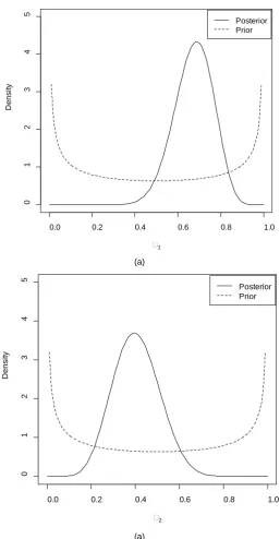
We note first that πˆ1=17 25=0.68, 8 20πˆ2 = =0.40, giving πˆ=0.28.

We obtain the prior and posterior distributions of π1 and π2 (Figure 1).

We wish to test:

0: 0.35 vs 1: 0.35

H π ≤ H π > (4)

We have α1 17.5, 8.5, 8.5, 12.5β1 α2 β2

∗₌ ∗ ₌ ∗ ₌ ∗ _{= :}

1

H has posterior

proba-bility

(

)

1

(

)

0.35

Pr π >0.35 =

∫

ψ x;17.5, 8.5, 8.5,12.5 dx=0.2855, and we fail to reject

0

H at the 0.05% level. This means that data combined with our judgment is not

enough to make us accept that the difference of these proportions exceeds 0.35. Naturally, different informative, or non-informative, priors can be considered for π1 and π2 separately, and the test can be carried out in the same way.

b) Point-null hypothesis:

The point null hypothesis H0:π η= vs. H1:π η≠ to be tested at the

(a)

[image:5.595.244.502.66.561.2]

(a)

Figure 1. (a) Prior Beta 0.5,0.5

(

)

and posterior Beta 17.5,8.5

(

)

of

1

π and (b) Prior Beta 0.5,0.5

(

)

and posterior Beta 8.5,12.5

(

)

of

2

π _.

in the literature. Several difficulties still remain concerning this case, especially on the prior probability assigned to the value η (see Berger [10]). We use here Lindley’s compromise (Lee [11]), which consists of computing the

(

1−α

)

100%

highest posterior density interval and accept or reject H0 depending on whether

η belongs or not to that interval. Here, for the same example, if η=0.35,

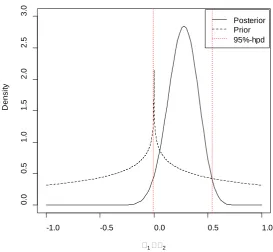
us-ing Pham-Gia and Turkkan’s algorithm [12], the 95% hpd interval for

π

is

(

−0.0079; 0.5381

)

, which leads us to technically accept H0 (see Figure 2),

al-0.0 0.2 0.4 0.6 0.8 1.0

0

1

2

3

4

5

₁

D

ens

it

y

Posterior Prior

0.0 0.2 0.4 0.6 0.8 1.0

0

1

2

3

4

5

2

D

ens

it

y

though the lower bound of the hpd interval can be considered as zero and we can practically reject H0.

We can see that the above conclusions on

π

_{are consistent with each other.}

3.2. Bayesian Testing Using the Bayes Factor

Bayesian hypothesis testing can also be carried out using the Bayes factor B, which would give the relative weight of the null hypothesis w.r.t. the alternative one, when data is taken into consideration. This factor is defined as the ratio of the posterior odds over the prior odds. With the above expression of the differ-ence of two betas given by (1) we can now accurately compute the Bayes factor associated with the difference of two proportions. We consider two cases:

a) Simple hypothesis: H0:π =a vs H1:π =b. Then

( )

( )

p a

B

p b

π

π π π

= _{, which}

corresponds to the value of the posterior density of

π

at a, divided by the

val-ue of posterior density of

π

at b. As an application, let us consider the

fol-lowing hypotheses (different from the previous numerical example):

0: 0.35

H π = vs. H1:π =0.25, where we have uniform priors for both π1 and 2

π _{, and where we consider the sampling results from Table 1. We obtain the} posterior parameters α1 18, 9, 9, 13β1 α2 β2

∗₌ ∗ ₌ ∗ ₌ ∗_{= . Using the density of the} difference (1), we calculate the Bayes factor,

(

)

(

11 11 22 22

)

0.35 , , ,

0.8416 0.25 , , ,

B

ψ α β α β

ψ α β α β

∗ ∗ ∗ ∗

∗ ∗ ∗ ∗

= = _{. This value indicates that the data slightly}

[image:6.595.236.510.437.689.2]

favor H1 over H0, which is a logical conclusion since πˆ=0.28.

Figure 2. Prior ψ

(

0.5,0.5,0.5,0.5

)

and posterior ψ

(

17.5,8.5,8.5,12.5

)

distributions of π. The red dashed lines correspond to the bounds of the posterior 95%-hpd interval.

-1.0 -0.5 0.0 0.5 1.0

0

.0

0

.5

1

.0

1

.5

2

.0

2

.5

3

.0

1 2

D

ens

it

y

Table 1. Data on customers in area A and B. Area

A B Combined Response

Response Yes 17 8 25

No 8 12 20

Totals 25 20 45

b) Composite hypothesis: As an application, let us consider the hypotheses (4), that is, H0:π ≤0.35 vs. H1:π >0.35.

In general, H0:π ∈ Θ0 vs. H1:π ∈ Θ1, where Θ ∪ Θ =0 1 R. We have

(

)

0 Pr 0posterior

p =

π

∈ Θ and p1=Pr

(

π

∈ Θ1posterior

)

(or p1= −1 p0) as

posterior probabilities. Consequently, we define the posterior odds on H0

against H1 as p0 p1. Similarly, we have the prior odds on H0 against H1,

which we define here as z0 z1. The Bayes factor is

0 1 1 0

p z B

p z

= _{. Again, we use the}

sampling results from Table 1, yielding the prior and posterior distributions presented in Figure 1 with Beta 0.5, 0.5

(

)

prior separately for both

propor-tions.

Now, using (4),

π ψ α β α β

(

1, 1, 2, 2

)

∗ ∗ ∗ ∗

∼ _{, we can determine the required prior}

and posterior probabilities. For example, 0 0.35

(

1 1 2 2

)

1

, , , d

p ψ α β α βt ∗ ∗ ∗ ∗ t

−

=

_∫

_gives

0 0.7145

p = . In the same way, we obtain z0=0.745, using the prior

(

1 2 ,1 2 ,1 2 ,1 2

)

ψ . Since p1= −1 p0 and z1= −1 z0, we have p1=0.2855

and z1=0.255. Finally, the Bayes factor is B=0.8566, which is a mild

argu-ment in favor of H1.

4. Prior and Posterior Densities of

π η

−

The testing above can be seen to be quite straightforward, and is limited to some numerical values of the function ψ

( )

. that can be numerically computed. But

to make an in-depth study of the Bayesian approach to the difference

(

)

1 2

π η π− = − π +η , we need to consider the analytic expressions of the prior and posterior distributions of this variable, which can be obtained only from the general beta distribution. Naturally, the related mathematical formulas become more complicated. But Pham-Gia and Turkkan [13] have also established the expression of the density of X1+X2, where both have general beta

distribu-tions.

4.1. The Difference of Two General Betas

The general beta (or GB), defined on a finite interval, say (c, d), has a density:

(

) (

) (

1

)

1

(

)

1

(

)

; , ; , , , , 0,

gb

f xα β c d = x−cα− d−x β− _ d−cα β+ − B α β _ α β > c≤ ≤x d (5)

and is denoted by X ~GB

(

α β, ; ,c d

)

. It reduces to the standard beta above

general beta by addition of, or/and, multiplication with a constant. Theorem 2: Let X ~GB

(

α β, ; ,a b

)

and any two scalars θ, λ. Then

1) X +θ~GB

(

α β, ;a+θ,b+θ

)

,

2) λX ~GB

(

α β λ λ, ; a, b

)

when λ >0. Otherwise, λX ~GB

(

β α λ λ, ; b, a

)

when λ <0.

Proof: 1) We have

( )

(

)

(

)

(

)

(

(

)

)

(

)

(

)

(

)

(

)

(

(

)

)

(

(

) (

)

)

(

)

1 1 1

1 1 1

, ,

, ,

X X

f y f y

y a b y b a B

a y b

y a b y b a B

a y b

θ

α β α β

α β α β

θ

θ θ α β

θ

θ θ θ θ α β

θ θ

+

− − + −

− − + −

= −

 

= − − − − _ − _

≤ − ≤

 

= − + + − _ + − + _

 

+ ≤ ≤ +

2) For λ >0,

( )

(

)

(

) (

)

(

)

(

)

(

) (

)

(

)

(

)

1 1 1

1 1

1

1

1

, ,

, ,

X X

f y f y

y a b y b a B a y b

y a b y b a B a y b

λ

α β α β

β α β

α λ λ

λ λ α β λ

λ

λ λ λ λ α β λ λ

− − + −

− + −

− =

 

= − − _ − _ ≤ ≤

 

= − − _ − _ ≤ ≤

When λ <0,

( )

(

)

(

) (

)

(

)

(

)

(

) (

)

(

)

(

)

1 1 1

1 1 1

1

1

, ,

, ,

X X

f y f y

y a b y b a B a y b

y b a y a b B b y a

λ

α β α β

β α α β

λ λ

λ λ α β λ

λ

λ λ λ λ α β λ λ

− − + −

− − + −

= −

 

= − − − _ − _ ≤ ≤

 

= − − _ − _ ≤ ≤

Q.E.D. Pham-Gia and Turkkan [13] gave the expression of the density of X1+X2,

where X1 and X2 are independent general beta variables. The density of

1 2

X −X , which is only mentioned there, is explicitly given below.

Proposition 2:

Let X1~GB

(

α β, ; ,c d

)

and X2 ~GB

(

γ δ, ; ,e f

)

. For the difference

1 2

X −X defined on

(

c− f d, −e

)

, there are two different cases to consider,

de-pending on the relative values of c−e and d− f , since X1 and X2 do not

have symmetrical roles. Case 1:

c− ≤ − ≤ − ≤ −f d f c e d e (6)

Case 2:

c− ≤ − ≤ − ≤ −f c e d f d e (7)

Theorem 3: Let X1 and X2 be two independent general betas with their

supports satisfying (6). Then Y =X1−X2 has its density defined as follows:

( )

(

(

)

)

(

)

(

)

(

)

(

) (

) (

)

(

)

(

)

(

)

1 1 1 1 , , ,

,1 ,1 ; ; ,

y c f d f y B

f y

d c f e B B

c f y y c f

F

d f y f e

α δ β

α β δ

δ α δ γ α β

δ β γ α δ

+ − − + − − − − − = − −  − − − −  − − +    _{− − −}    (8)

For d− ≤ ≤ −f y c e,

( )

(

(

)

)

(

)

(

)

(

)

(

)

1 1 1 1 ,

,1 ,1 ; ; ,

y d f d e y

f y

f e B

c d d c

F

y d f d e y

δ γ

δ γ _{δ γ}

β δ γ α β

− − + − − + − − = −  _{− − +} − −     _{− − − −}    (9)

and for c− ≤ ≤ −e y d e,

( ) (

(

)

)

(

(

)

)

(

)

(

) (

)

(

) (

)

(

)

(

)

(

)

1 1 1 1 , , ,

,1 ,1 ; ; ,

d e y y d f B

f y

d c f e B B

d e y y d e

F

d c y d f

β γ δ

β δ γ

β γ δ γ α β

β α δ β γ

+ − − + − − − − − = − −  − − − −  − − +    _{− − −}    (10)

where F1

( )

. is Appell’s first hypergeometric function already discussed.

Proof:

The argument uses first part 2) of Theorem 1 to obtain that

(

)

2 ~ , ; ,

X GB δ γ f e

− − − . Then, it uses the exact expression of the density of the sum of two general betas (see Theorem 2 in the article of T. Pham-Gia & N. Turkkan [14]).

Q.E.D. We denote the above density given by (8), (9) and (10) by

(

1, 1, 2, 2; , , ,c d e f

)

π

ϕ α β α β

Note: The corresponding case 2, when relation (7) is satisfied, is given in Ap-pendix 1 (Theorem 3a).

To study the density of π η π− = 1−

(

π2+η

)

, a particular case that will be

used in our study here is the difference between X1 ~GB

(

α β1, 1; 0,1

)

and

(

)

2 ~ 2, 2; , 1 , 1 1

X GB α β η η+ − ≤ ≤η , with η being a positive constant.

In this case both Theorem 2 and Theorem 3 apply since c− = −e d f and

the middle definition section of ϕ α β α βπ

(

1, 1, 2, 2; , , ,c d e f

)

disappears.

Theorem 4: Let X1~GB

(

α β1, 1; 0,1

)

and X2 ~GB

(

α β η η +2, 2; , 1

)

be two

independent general beta distributed random variables. Then the density of

1 2

Y =X −X , defined on _−

(

η

+1 ,1

)

−

η

_, is:

1)

for − − ≤ ≤ −η 1 y η,

( )

(

(

)

)

₍

(

_{) (}

)

₎

(

)

(

)

₍

₎

1 21 21

1 2

1 1 2 2

1 2 1 2 1 2

1 ,

, ,

1

,1 ,1 ; ; , 1

y y B

f y

B B

y

F y

y

α β α

η η α β

α β α β

η

β β α α β η

η + − − + + − − = + +   − − + + +  ₊   

( ) (

(

)

)

₍

(

_{) (}

)

₎

(

)

(

)

(

)

2 11 21

2 1

1 1 2 2

1 1 1 2 2 1

1 ,

, ,

1 ,1 ,1 ; ; 1 ,

y y B

f y

B B

y

F y

y

α β β

η η α β

α β α β

η

β α β α β η

η + − − − − + = − −   − − + − −  ₊   

and we denote this distribution by

(

1 1 2 2

)

~ , , , ;

Y ξ α β α β ηη . (11) Proof:

This is a special case of Theorem 3.

Q.E.D. An equivalent form using Theorem 4 leads to a slightly different expression, which gives however, the same numerical values for the density of π η− (see Theorem 4a in Appendix 1).

4.2. Prior and Posterior Distributions of

π η

−

Let πi, 1, 2i= be two independent beta distributed random variables, the first

being a regular beta, π1~ beta

(

α β1, 1

)

, and the second being a general beta,

(

)

2~GB 2, 2; ,1

π α β η +η _.

Binomial sampling, with these two different beta priors, leads to the following Proposition 3: The prior distribution of π η π− = 1−

(

π2+η

)

is

(

1, 1, 2, 2;

)

η

ξ α β α β η , given by (11), and its posterior distribution is

(

1, 1, 2, 2;

)

η

ξ α β α β η

∗ ∗ ∗ ∗ _with

i i xi α∗ ₌α _{+ and}

, 1, 2. i i ni xi i β∗₌β _{+ − =} Proof:

(

)

1 2

π − π +η is the difference of two random variables with respective distri-bution beta

(

α β1, 1

)

and GB

(

α2,β2; ,ηη+1

)

, The prior distributions of π η−

is hence ξ α β α β ηη

(

1, 1, 2, 2;

)

, as given by (14).

Binomial sampling affects these 2 distributions in different ways. For the first, the posterior is beta

(

α1+x1,β1+ −n1 x1

)

while the posterior distribution of the

second is GB

(

α2+x2,β2+n2−x2; ,ηη+1

)

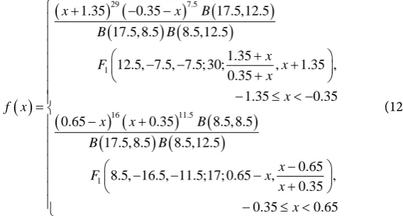
(see Proposition 3a in Appendix

2). Figure 3 shows the prior and the posterior of π +2 0.35.

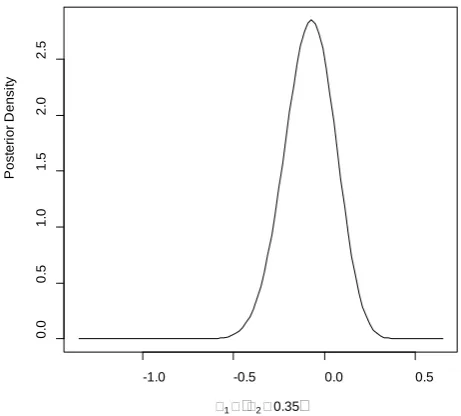
From Theorem 4, we obtain the expression of the posterior density

(

)

.35 17.5,8.5,8.5,12.5; 0.35

ξ of π η− as follows:

( )

(

) (

)

(

)

(

) (

)

(

) (

)

(

)

29 7.5 1 16 11.5

1.35 0.35 17.5,12.5

17.5, 8.5 8.5,12.5

1.35

12.5, 7.5, 7.5; 30; , 1.35 ,

0.35

1.35 0.35

0.65 0.35 8.5, 8.5

17.

x x B

B B x F x x x f x

x x B

B + − − +  _{− − +}   ₊   

− ≤ < − =

− +

(

) (

)

1

5, 8.5 8.5,12.5

0.65

8.5, 16.5, 11.5;17; 0.65 , ,

0.35 0.35 0.65 B x F x x x              _{ − } − − −  _{ } +   

 _{− ≤ <}



[image:10.595.251.535.562.717.2]

(12)

(a)

[image:11.595.237.506.70.580.2]

(b)

Figure 3. (a) Prior GB

(

0.5,0.5,0.35,1.35

)

distribution of π2+0.35 and

(b) Posterior GB

(

8.5,12.5;0.35,1.35

)

distribution of π₂+0.35. The posterior of π1−

(

π2+η

)

is hence given by Theorem 4, as

(

1, 1, 2, 2;

)

η

ξ α β α β η∗ ∗ ∗ ∗ _.

5. Conclusion

The Bayesian approach to testing the difference of two independent propor-tions leads to interesting results which agree with frequentist results when non-informative priors are considered. Undoubtedly, all preceding results can be

0.4 0.6 0.8 1.0 1.2

0

1

2

3

4

20.35

P

ri

or

D

ens

it

y

0.4 0.6 0.8 1.0 1.2

0

1

2

3

4

20.35

P

os

ter

ior

D

ens

it

[image:12.595.257.488.70.278.2]

Figure 4. Posterior density ξ.35

(

17.5,8.5,8.5,12.5;0.35

)

of

(

)

1 2 0.35

π − π + .

generalized to other measures frequently used in a 2 × _{2 table.}

Acknowledgements

Research partially supported by NSERC grant 9249 (Canada). The authors wish to thank the Universite de Moncton Faculty of Graduate Studies and Research for the assistance provided while conducting this work.

References

[1] Pham-Gia, T. and Turkkan, N. (1993) Bayesian Analysis of the Difference of two Proportions. Communications in Statistics—Theory and Methods, 22, 1755-1771. https://doi.org/10.1080/03610929308831114

[2] Pham-Gia, T. and Turkkan, N. (2008) Bayesian Analysis of a 2 × 2 Contingency Ta-ble with Dependent Proportions and Exact Sample Sizes. Statistics, 42, 127-147. https://doi.org/10.1080/02331880701600380

[3] Pham-Gia, T. and Turkkan, N. (2003) Determination of the Exact Sample Sizes in the Bayesian Estimation of the Difference between Two Proportions. Journal of the Royal Statistical Society,52, 131-150. https://doi.org/10.1111/1467-9884.00347 [4] D’Agostino, R., Chase, W. and Belanger, A. (1988) The Appropriateness of Some

Common Procedures for Testing the Equality of Two Independent Binomial Popu-lations. The American Statistician, 42, 198-202.

[5] Cressie, N. (1978) Testing the Equality of Two Binomial Proportions. Annals of the Institute of Statistical Mathematics, 30, 421-427.

https://doi.org/10.1007/BF02480232

[6] Eberhardt, K.R. and Fligner, M.A. (1977) A Comparison of Two Tests for Equality of Two Proportions. The American Statistician, 21, 151-155.

https://doi.org/10.1080/00031305.1977.10479225

[7] Santner, T.J. and Snell, M.K. (1975) Small Sample Confidence Intervals for p1−p2

and p p1 2 in 2 × 2 Contingency Tables. JASA, 75, 386-394.

-1.0 -0.5 0.0 0.5

0

.0

0

.5

1

.0

1

.5

2

.0

2

.5

120.35

P

os

ter

ior

D

ens

it

[8] Howard, J.V. (1998) The 2 × 2 Table: A Discussion from a Bayesian Viewpoint. Sta-tistical Sciences, 13, 351-367. https://doi.org/10.1214/ss/1028905830

[9] Agresti, A. and Coull, B. (1998) Approximate Is Better than Exact for Interval Esti-mation of Binomial Proportions. The American Statistician, 52, 2.

[10] Berger, J. (1999) Bayes Factor. In: Kotz, S., Read, C.B. and Banks, D.L., Eds., Encyc-lopedia of Statistics, Update 3, Wiley, NY, 20-29.

[11] Lee, P.M. (2004) Bayesian Statistics.An Introduction. 3rd Edition, Hodder Arnold, London.

[12] Pham-Gia, T. and Turkkan, N. (1993) Computation of the Highest Posterior Den-sity Interval in Bayesian Analysis. Journal of Statistical Computation and Simula-tion, 44, 243-250. https://doi.org/10.1080/00949659308811461

[13] Pham-Gia, T. and Turkkan, N. (1998) Distribution of the Linear Combination of Two General Beta Variables and Applications. Communications in Statistics—Theory and Methods, 27, 1851-1869. https://doi.org/10.1080/03610929808832194

Appendix 1

Below is the expression of the density of Y =X1−X2 when (7) is satisfied,

in-stead of (6). This expression, with the one given in Theorem 3, covers all cases. Theorem 3a: Let X1 and X2 be two independent general betas with their

supports satisfying (10). Then Y =X1−X2 has its density defined as follows:

for c− ≤ ≤ −f y c e,

( )

(

(

)

)

(

)

(

)

(

)

(

) (

) (

)

(

)

(

)

(

)

1 1 1 1 , , ,

,1 ,1 ; ; ,

y c f c e y B

f y

f e d c B B

c f y y c f

F

c e y d c

α δ γ

δ γ α

α δ α β δ γ

α γ β α δ

+ − − + − − − − − = − −  − − − −  − − +    _{− − −}    (13)

For c− ≤ ≤ −e y d f,

( )

(

(

)

)

(

)

(

)

(

)

(

)

1 1

1

1 ,1 ,1 ; ; ,

,

y c e d e y e f f e

f y F

y c e d e y

d c B

α β

α β _{α β} γ α β δ γ

− −

+ −

+ + − −  − − 

= _ − − + _{− − − −} _

−   (14)

For d− ≤ ≤ −f y d e,

( ) (

(

)

)

(

(

)

)

(

)

(

) (

)

(

) (

)

(

)

(

)

1 1 1 1 , , ,

,1 ,1 ; ; ,

d e y y c e B

f y

f e d c B B

d e y y d e F

f e y

β γ α

γ α β

β γ δ γ α β

γ δ α β γ

+ − − + − − − − − = − − − − − −   − − +  ₋    (15) Proof:

By rewriting Y = −

(

X2

) (

− −X1

)

, we can apply the above Theorem 2 and

Theorem 3.

Q.E.D A parallel, and equivalent, result to Theorem 4 is given below:

Theorem 4a: The density of X1−X2−η is:

For − − ≤ ≤ −η 1 y η,

( )

(

(

)

)

₍

(

_{) (}

)

₎

(

)

(

)

₍

₎

1 21 21

1 2

1 1 2 2

1 1 2 1 1 2

1 ,

, ,

1

,1 ,1 ; ; , 1

y y B

f y

B B

y

F y

y

α β α

η η α β

α β α β

η

α α β α β η

η + − − + + − − = + +   − − + + +  ₊   

For − ≤ ≤ −η y 1 η,

( ) (

(

)

₍

)

_{) (}

(

)

₎

(

)

(

)

(

)

2 11 11

2 1

1 1 2 2

1 2 2 1 2 1

1 ,

, ,

1

,1 ,1 ; ; 1 ,

y y B

f y

B B

y

F y

y

α β α

µ η α β

α β α β

η

α β α α β η

η + − − − − + = − −   − − + − −  ₊   

and we denote Y ~ξ α β α β ηη

(

1, 1, 2, 2;

)

∗ _.

Proof:

Similar to the proof of Theorem 4.

Appendix 2

Proposition 3a:

Suppose that X2~ Bin

(

n2,π2

)

and π2 has the prior distribution

(

2 2

)

beta α β, then the posterior distribution of π2+η is

(

2 x2, 2 n2 x2; , 1

)

GB α + β + − ηη+ .

Proof:

The prior distribution of π2+η is GB

(

α β η η +2, 2; , 1

)

(see Theorem 2) with

the pdf

(

)

(

) (

) (

2

)

2

2

1 1 1

2 2 2, 2 2 1 2 , 12

f_{π η}+ π x =B α β − π −η α− + −η π β− η π≤ ≤ +η ,

The likelihood function is

(

)

(

)

2

(

)

2 2

2 2 2 2

2

2 2 2 2 2 2

2

1 n x , 0,1, ,

x

X X

n

f x f x x n

x

π η θ π π π π

− +

 

= =_{ } − =

  

Thus the marginal distribution of X2, the number of success, with π2= −θ η,

has density:

(

)

₍

₎

(

) (

)

(

)

(

)

(

) (

) (

) (

)

(

)

(

)

(

)

(

)

2 2 2 2 2

2 2 2 2 2

2 2 2 2 2

2

1 1 1

2

2 2 2 2

2 2 2

1 1 1

2 2 2

2

1 1 1

2 2 2

2 2

2 2 2

2 2

2 , 2 1 1 d

,

1 1 d

, , , , 1 d , , n x x

x n x

x n x

n x B n x B n x B n x x

K x n

B B

η α β

η

η α β

η

η α β

η

α β θ η η θ π π θ

α β

θ η η θ θ η η θ θ

α β

θ η η θ θ

α β α β α β + − − − + − − − + + − + − − = = = =       _{− + − −}       _{− + − − + −}       _{− + −}       _{+ +}

∫

∫

∫

(

n2−x2

)

Therefore, the posterior distribution of θ _given X₂=x₂ is

(

)

(

₍

)

(

₎

)

(

) (

) (

)

(

)

(

) (

)

(

)

(

)

(

)

2 2 2

2 2

2 2 2 2 2

2 2 2 2 2

2 2

2

2 2

1 1 1 2

2 2 2 2

2

2 2

2 2

2 2 2 2 2

2 2 2

1 1

2 2 2 2 2

, , 1 , , , wit 1 ,

, 1

1 , 1 h , X X n x x

x n x

f x f x

f x n B x n x K x

x n x

B x n n B B x π η π η α β π β η α θ θ θ α β

α β θ η η θ π π

α β

α β

π θ η η θ η

θ η η θ _{η θ η}

α β + + − − − + − + − + − − =   − + − −   _{ }     =       _{+ −} = − ≤ ≤ + − + − = ≤ − + + ≤ + +

This is the p.d.f. of GB

(

α2+x2,β2+n2−x2; ,ηη+1

)

.

Submit or recommend next manuscript to SCIRP and we will provide best service for you:

Accepting pre-submission inquiries through Email, Facebook, LinkedIn, Twitter, etc. A wide selection of journals (inclusive of 9 subjects, more than 200 journals)

Providing 24-hour high-quality service User-friendly online submission system Fair and swift peer-review system

Efficient typesetting and proofreading procedure

Display of the result of downloads and visits, as well as the number of cited articles Maximum dissemination of your research work