Munich Personal RePEc Archive
Testing for predictability in a
noninvertible ARMA model
Lanne, Markku and Meitz, Mika and Saikkonen, Pentti
2012
Online at
https://mpra.ub.uni-muenchen.de/37151/
1
Introduction
Testing for autocorrelation or predictability in time series data has attracted considerable in-terest in various …elds of application. A prominent example is testing the predictability of asset returns which has rather a long history in empirical …nance (see Campbell, Lo, and MacKinlay (1997, Ch. 2)). As serial correlation in asset returns is weak at best, tests based directly on the sample autocorrelation function tend to lack power, and testing has, in addition, been based on time series processes implied by structural models. Amongst these, the …rst-order autoregres-sive moving average (ARMA(1,1)) process implied by the price-trend model of Taylor (1982) and the mean-reversion model of Poterba and Summers (1988) has been in‡uential.
As a starting point both Andrews and Ploberger (1996) and Nankervis and Savin (2010) have the stationary and invertible ARMA(1,1) model
yt= 0yt 1+"t #0"t 1; (1)
where the parameters 0 and #0 satisfy j 0j < 1 and j#0j < 1, and "t is an uncorrelated zero
mean error term, that is, white noise. For testing purposes the model is reparameterized as
yt = (#0+ 0)yt 1+"t #0"t 1;
where 0 = 0 #0. The null hypothesis of interest is thatytis white noise or that 0 = 0. As
the null hypothesis implies that yt = "t, the nuisance parameter #0 is present only under the
alternative, explaining why the testing problem is nonstandard (cf. Davies (1977)).
Based on a Gaussian likelihood Andrews and Ploberger (1996) show that their likelihood ratio (LR) test and so-called supremum Lagrange multiplier (LM) tests and average exponential LM tests have desirable asymptotic properties, and they justify the asymptotic distributions of these tests without invoking Gaussianity and independence that were initially used to motivate the tests. Nankervis and Savin (2010) modify (some of) the tests of Andrews and Ploberger (1996) to make them applicable to a wider range of data generation processes. Using a gen-eral near epoch dependence assumption, they develop sevgen-eral test statistics with the same asymptotic distributions as the corresponding tests statistics of Andrews and Ploberger (1996). Unlike the tests of Andrews and Ploberger (1996), those of Nankervis and Savin (2010) are valid for data that are uncorrelated but dependent exhibiting, for instance, ARCH type conditional heteroskedasticity.
A noninvertible version of the ARMA(1,1) model (1) is obtained by assuming j#0j > 1
instead of j#0j < 1. Asymptotic estimation theory of this kind of ARMA models has been
not consider noncausal ARMA models in this paper. Some of the recent work on the estimation of noninvertible ARMA models has been focused on so-called all-pass models which in the …rst order (causal) case are obtained from (1) by imposing the restriction 0 = 1=#0 (j#0j>1) (see
Breidt, Davis, and Trindade (2001) and Andrews, Davis, and Breidt (2006, 2007)). From the viewpoint of testing for serial correlation, all-pass processes are interesting in that they can generate time series that are uncorrelated but dependent. This is a useful feature in testing for predictability as it facilitates detecting nonlinear dependence in case no autocorrelation is found. However, as already indicated the dependence of an all-pass process requires non-Gaussian data which is also required in the estimation theory discussed above as well as in the tests developed in this paper (see the aforementioned references and the discussion in the next section).
The LR and Wald tests to be derived in this paper are not directly based on the formu-lation of the noninvertible ARMA(1,1) model discussed in the preceding paragraph and the references therein. Instead, we use a formulation similar to that in Meitz and Saikkonen (2011) where parameter estimation in a noninvertible ARMA model with autoregressive conditionally heteroskedastic errors is studied. The reason for this is the fact that while assumingj#0j>1in
(1) makes the model noninvertible, it also complicates the derivation of the tests. This can be seen by noticing that in (1)j 0j<1is assumed and the null hypothesis 0 = 0 can equivalently
be stated as 0 =#0, provided j#0j>1 is not assumed. In addition to a general noninvertible
ARMA model we also consider tests within the corresponding all-pass model. Due to the afore-mentioned reasons of identi…cation, our theoretical results assume a general non-Gaussian error distribution. In the empirical application of the paper, Student’st–distribution is employed.
predictable. The tests of Nankervis and Savin (2010) agree on the absence of autocorrelation, but they have little to say about predictability in general.
The remainder of the paper is organized as follows. Section 2 introduces our formulation of the noninvertible ARMA(1,1) model and discusses its properties. The test procedures are derived in Section 3 and studied by means of Monte Carlo simulation experiments in Section 4. An empirical application to testing the predictability of U.S. stock returns is presented in Section 5. Finally, Section 6 concludes. Some technical details are deferred to Appendices.
2
Noninvertible ARMA(1,1) and all-pass models
In this section, we discuss our formulation of the noninvertible ARMA(1,1) model, and its special case the all-pass model, in some detail. We de…ne our noninvertible ARMA(1,1) model by the equation
yt= 0yt 1+ t 1 0 t; (2)
where 0 and 0 are parameters satisfying j 0j < 1 and j 0j < 1, and t is an uncorrelated
error term with zero mean and …nite variance 2
0. (Throughout the paper, a subscript zero
signi…es a true (but unknown) parameter value.) LettingB denote the backward shift operator
(Bk t= t k,k = 0; 1; 2; : : :) we can write equation (2) as
(1 0B)yt= (1 0B 1)B t. (3)
When 0 6= 0, the connection between the speci…cations (1) and (2) is given by 0 = 1=#0 and
t= #0"t; when 0 = 0, the moving average part in (2) reduces to the uncorrelated error term
t 1, and the same is achieved in (1) by setting #0 = 0 and "t= t 1.
function of the noninvertible ARMA(1,1) process yt in (2) can be seen to equal 2
0 2
j(1 0ei!)e i!j2
j1 0e i!j2 = 2 0 2
j1 0e i!j2
j1 0e i!j2: (4)
The right-hand side of (4) coincides with the spectral density function of a conventional invert-ible ARMA(1,1) process with the same parameter values as in (2). This means that invertinvert-ible and noninvertible ARMA processes cannot be distinguished by the spectral density function and, hence, by the autocovariance function. As the Gaussian likelihood function of an ARMA model is determined by the autocovariance function of the observed process, it also becomes understandable why estimation and statistical testing in noninvertible ARMA models assumes a non-Gaussian data generation process (in our case, a speci…c reason is that the information matrix based on a Gaussian likelihood becomes singular under the considered null hypotheses, as demonstrated in Appendix C). Known results on maximum likelihood (ML) and quasi ML estimation of noninvertible ARMA models also require that the error term is independent and identically distributed (IID). Unless otherwise stated we shall therefore assume that the error term t in our model (2) is non-Gaussian and IID.
An interesting special case of the noninvertible ARMA(1,1) model (2) is obtained when
0 = 0. In this case, the process is called an all-pass process and de…ned as
yt= 0yt 1+ t 1 0 t; (5)
where j 0j < 1 and t is non-Gaussian and IID, as in (2). All-pass processes are uncorrelated
(the spectral density in (4) reduces to 2
0=2 when 0 = 0), but dependent (note that in (3)
the operators 1 0B and 1 0B 1 do not cancel out even when 0 = 0). It may be worth
noting, however, that, even though uncorrelated, all-pass processes are in general predictable. A formal justi…cation for this fact is given in Appendix A, where it is demonstrated that the best (in mean square error sense) predictor of a (non-Gaussian) all-pass process is nonzero.
The same holds true for noninvertible ARMA models in general. In Appendix A we derive the autocorrelation function of squared observations from a noninvertible ARMA(1,1) process,
Cor(y2
t; y2t+k), and from the expression therein it can be seen that for non-Gaussian errors one
may expect to observe autocorrelation in squared observations generated by a noninvertible ARMA(1,1) process or an all-pass process. For certain values of the parameters 0 and 0,
the autocorrelation in squared observations can be quite strong. This happens especially when the signs of 0 and 0 are di¤erent in which case the …rst order autocorrelation can even be
close to unity. In such cases the series itself is also autocorrelated so that the situation is di¤erent from that in (pure) GARCH processes. In the all-pass process, the autocorrelation in squared observations is always rather mild, indicating that it may not be appropriate, say, for frequently observed …nancial time series which are typically (nearly) uncorrelated and exhibit strong conditional heteroskedasticity.
As a remark, we also note that if an invertible ARMA model is …tted to a time series generated by a (non-Gaussian) noninvertible ARMA process, the resulting squared residuals tend to be autocorrelated. To see this, write equation (3) as
(1 0B)yt= (1 0B) t; t=
(1 0B 1) (1 0B)
B t;
where t is an all-pass process. Thus, when 0 6= 0, the errors t are uncorrelated but, as
discussed in the previous paragraph, their squares are generally correlated.
We close this section by introducing the hypotheses we are interested in testing within the noninvertible ARMA(1,1) model (2) or the all-pass model (5). As there are more than one hypothesis, some kind of a sequential approach may be employed. One possibility is to start from the totally unrestricted model and test whether it reduces to an all-pass model. The hypothesis of interest is then
HA P : 0 = 0 in model (2).
The alternative is 0 6= 0. If this hypothesis is rejected the conclusion is that the process
parameters 0 and 0 is zero in which case the observed process is IID. For studying this, the
relevant hypothesis is
H(A P )
I ID : 0 = 0 in model (5)
with the alternative being 0 6= 0. In this case, a rejection means that the process is
uncor-related but dependent and (nonlinearly) predictable, whereas a nonrejection supports the IID hypothesis.
If the IID process is a priori highly plausible, it may be a good idea to test for the IID hypothesis
HI ID : 0 = 0 = 0 in model (2)
directly within the unrestricted noninvertible ARMA(1,1) model. If a rejection results, the relevant hypothesis to test next is the all-pass hypothesis HA P. However, according to our
simulation experiments in Section 4 the LR and Wald tests of the IID hypothesis HI ID may
have relatively low power against close alternatives, suggesting that slight deviations from independence may not be detected. Therefore, if on a priori grounds the IID hypothesis is implausible, it may be advisable to start out with the all-pass hypothesis HA P so as not to
dismiss potential weak nonlinear dependence. For instance, in testing the predictability of asset returns, the general wisdom seems to be that the IID hypothesis is very unlikely to hold so that the all-pass hypothesis should be more interesting than the IID hypothesis.
As already discussed, all-pass processes exhibit ARCH-type dependence in the form of correlation in the squared observations. In this respect, our assumption of the error term t
independence although this may not be such a serious shortcoming, if the IID assumption can be precluded as incredible as seems to be the case in certain applications.
3
Test procedures
We now formulate (approximate) Wald and LR tests for the hypotheses introduced in the previous section. We start with a brief discussion of the assumptions needed.
We have already assumed the error term t to be non-Gaussian and IID. Assume further
that t has a continuous distribution with a density function f 0(x; 0) =
1
0 f 01x; 0 that
may also depend on the parameter vector 0 (d 1) in addition to the scale parameter 0.
For our theoretical developments, the function f(x; ) has to satisfy a number of regularity conditions similar to those used in related previous work on noninvertible and noncausal ARMA models (see Breidt et al. (1991), Lii and Rosenblatt (1996), Andrews, Davis, and Breidt (2006), and Lanne and Saikkonen (2011)). These conditions are technical in nature, and we relegate their precise formulation to Appendix C, where further discussion is also provided. Here we only note that the required conditions are satis…ed by several conventional distributions such as the (rescaled) Student’st–distribution and weighted averages of Gaussian distributions. Their exact formulation is adopted from a recent paper by Meitz and Saikkonen (2011) where an asymptotic estimation theory for noninvertible ARMA models is extended to allow for ARCH type conditional heteroskedasticity. In the present context, the assumptions used in Meitz and Saikkonen (2011) are convenient because, unlike in other related previous work, the formulation of the employed noninvertible ARMA model is similar to (2). On the other hand, because some of these assumptions were originally designed to deal with conditional heteroskedasticity they may be unnecessarily strong in our context. However, as the main focus of our paper is to present a new approach of testing for autocorrelation and predictability, no attempt is made to …nd the weakest possible assumptions.
permissible parameter space is given by j j < 1, j j < 1, > 0, and 2 where Rd.
Suppose that observationsy0; : : : ; yT are available. We estimate the parameters by maximizing
the approximate log-likelihood function (divided by T)
~
LT( ) =T 1 T
X
t=1
logf ~t 1( ); 1 2log
2
the derivation of which is discussed in some detail in Appendix B. Here we only note that the quantities~T 1( ); : : : ;~0( ) are solved by using the backward recursion
~t 1( ) =yt yt 1+ ~t( ); t=T; : : : ;1;
with end condition ~T( ) = 0. It is demonstrated in Appendix C that, under the regularity conditions stated therein, the approximate log-likelihood functionL~T( )has a (local) maximizer ~which is consistent and asymptotically normally distributed. Speci…cally, we have
p
T(~ 0)!d N(0;I( 0) 1) as T ! 1;
where the positive de…nite matrix I( 0) is de…ned in Appendix C. Here it su¢ces to note that a consistent estimator of I( 0) is obtained in the usual way from the Hessian of the log-likelihood function (but not from the outer product of the score matrix). Thus, denoting
JT( ) = @2L~T( )=@ @ 0 we haveJT(~) p
! I( 0).
The preceding discussion can readily be modi…ed to concern estimation of parameters of the all-pass model (5). It su¢ces to rede…ne = ( ; ; )and compute~t 1( ) in the approximate
log-likelihood functionL~T( )with the restriction = . The asymptotic normality result of the
obtained estimator then applies with a consistent estimator of the limiting covariance matrix de…ned in terms of the Hessian of the employed counterpart of L~T( ).
Based on the preceding results we can derive Wald and LR tests for the hypotheses intro-duced in the preceding section. First consider the all-pass hypothesis HA P and partition the
parameter vector as = ( 1; 2), where 1 = ( ; ) and 2 = ( ; ). Let ~ = (~1;~2) and
matrix JT(~). To simplify notation, we denoteJ~ij =J i j;T(~)(i; j = 1;2). Then, de…ning the
vectora = (1; 1)we can write the Wald test statistic for HA P as
WA P =T~
0
1a a
0
( ~J11 J~12J~221J~21) 1a 1
a0~
1 d
! 21 under HA P:
Of course, one can alternatively obtain a Wald test with asymptotic standard normal distrib-ution. For the corresponding likelihood ratio test, let~A P = (~A P;~A P;~A P;~A P) signify the ML
estimator of 0 constrained by HA P. Then, the LR test statistic for testingHA P reads as
LRA P = 2T L~T(~) L~T(~A P) d
! 21 under HA P:
Obtaining a Wald test for the IID hypothesis H(A P )I ID with a standard normal limiting
dis-tribution is simple. The test statistic is just the estimator ~A P divided by its approximate
standard error obtained from the square root of the …rst diagonal element of the inverse of the relevant Hessian discussed above. For the corresponding LR test one needs to estimate the nuisance parameters 0 and 0, that is, maximize the likelihood function de…ned by assuming
that the observed seriesyt,t= 0; : : : ; T, is IID with marginal distribution characterized by the
density f 0(x; 0). Denoting the resulting restricted estimator of the parameter vector 0 by
~I ID = (0;0;~I ID;~I ID) we get the LR test statistic
LR(A P )
I ID = 2T L~T(~A P) L~T(~I ID) d
! 21 under H (A P ) I ID :
Along the same lines one can also construct a test for the IID hypothesis HI ID. The Wald
test statistic can be formed by replacing the vector a in test statistic WA P by a2 2 identity
matrix whereas the corresponding LR test statistic can be formed by replacing the estimator
~A P in test statisticLRA P by the estimator~I ID. Both of these test statistics have an asymptotic 2
2 distribution under the null hypothesis.
ARMA(1,1) model. Then a non-standard testing problem with complicated limiting distribu-tions results because a nuisance parameter is present in the model only under the alternative hypothesis; see Andrews and Ploberger (1996) and Nankervis and Savin (2010).
4
Simulation study
In this section, we explore the …nite-sample properties of the proposed tests by means of Monte Carlo simulation experiments. In addition to reporting the results of a number of size and power simulations of the Wald and LR tests, we also simulated the tests of Nankervis and Savin (2010) for comparison. The new tests are shown to be superior in testing the null hypothesis of no autocorrelation against the noninvertible ARMA(1,1) process. Throughout the results are based on 10,000 replications, and two sample sizes, 200 and 500, are considered.
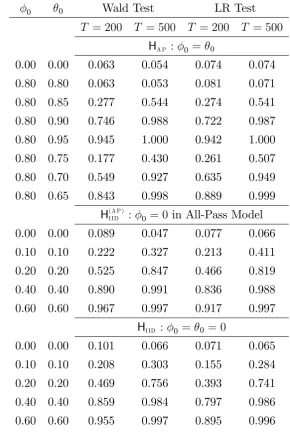
Table 1 presents the rejection rates of the 5% level Wald and LR tests, when the data are generated from the noninvertible ARMA(1,1) model with the error term having Student’s t– distribution with 5 degrees of freedom (this error distribution is also used in other simulation experiments discussed in this section). As far as the all-pass hypothesisHA P in the noninvertible
ARMA(1,1) model is concerned, the size of the Wald test seems to be closer to the nominal size than that of the LR test. In order to study the power of the tests, we consider alternative data generation processes with 0 …xed at 0.8 and and 0 taking values between 0.85 and 0.65.
Comparable parameter values are likely to be encountered in typical empirical applications of these tests. The rejection rates of both tests increase as a function of the distance of 0
from 0.8, with an equal distance resulting in greater empirical power when 0 exceeds 0.8. In
general, both tests have good power compared to the tests of Nankervis and Savin (2010) (to be discussed in more detail below), and the di¤erences between them are minor.
The rejection rates of the Wald and LR tests for the IID hypothesis H(A P )I ID in the all-pass
rates lie close to the nominal size. The empirical power is reasonable already for relatively small deviations from the null hypothesis, and it increases steadily with the parameter values. The di¤erences between the Wald and LR tests are minor.
The lower panel of Table 1 presents the rejection rates of the Wald and LR tests for the IID hypothesisHI ID in the noninvertible ARMA(1,1) model. In accordance with the tests of the IID
hypothesisH(A P )I ID in the all-pass model, both tests tend to overreject with only 200 observations,
with the overrejection problem relieved as the sample size increases. With 200 observations, the size of the Wald test is more seriously distorted, but at the greater sample size, the di¤erence between the tests is negligible. The power properties of the tests developed for the hypotheses
HI ID and H (A P )
I ID are similar but the latter seem to be superior, especially at alternatives close
to the null hypothesis. This suggests that it might be preferable to test for independence in the all-pass model instead of the unrestricted noninvertible ARMA(1,1) model, provided the all-pass restriction is not rejected.
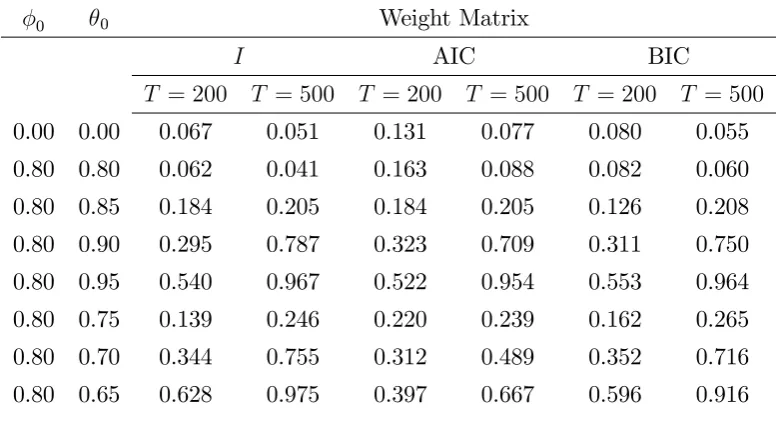
For comparison, in Table 2, we report the rejection rates of the Exp-LM1test of Nankervis
and Savin (2010), which is the one of their tests that they recommend for nonseasonal applica-tions in economics and …nance. As the null hypothesis of these tests is that of no autocorrelation, they should be compared to our tests of the all-pass hypothesisHA P. The …nite-sample behavior
of their sup LM and Exp-LM0 tests is similar in our setup (to save space the results are not
with as many as 500 observations. As far as power is concerned, qualitatively the …ndings are similar to those for the tests of the all-pass hypothesis HA P in the upper panel of Table 1, but
in each case the Exp-LM1 test is beaten by our Wald and LR tests by a considerable margin.
For instance, when 0 = 0:9 and T = 200, the Wald and Exp-LM1 tests reject approximately
75% and 30% of the time, respectively, with both tests su¤ering from small size distortions of similar magnitude. This indicates that for testing for serial correlation in the noninvertible ARMA model, the new tests are clearly superior to the those of Nankervis and Savin (2010), especially when autocorrelation is relatively weak.
As discussed in Section 2, when the values of 0 and 0 are very di¤erent, the noninvertible
ARMA(1,1) process can exhibit even strong ARCH-type dependence. Hence, it is plausible that our tests have some power against serially uncorrelated GARCH processes, i.e., they may reject the all-pass hypothesisHA P although the series is not autocorrelated but strongly conditionally
heteroskedastic. It is worth noting, however, that there are no statistical reasons why our tests should maintain their size in cases like these which are outside the model class assumed to derive the tests.
To check how sensitive our tests are to ARCH-type dependence we ran simulations with the GARCH(1,1) model as the data generation process. We used the same parameter values as Nankervis and Savin (2010) did in their simulations, but instead of Gaussian errors, we gen-erated errors from Student’s t–distribution with 5 degrees of freedom. The parameter values of Nankervis and Savin (2010) imply rather strong ARCH e¤ects, and, not surprisingly, our tests have nonnegligible, but relatively low power against this data generation process. The rejection rates of the Wald test of the all-pass hypothesis HA P equal 0:13 and 0:15 with 200
and 500 observations, respectively. With the LR test the corresponding …gures are higher,0:19
het-eroskedasticity. Therefore, the tests cannot without reservation be recommended for frequently sampled …nancial time series exhibiting strong conditional heteroskedasticity.
5
Empirical application
As pointed out in the Introduction, testing the predictability of asset returns continues to be an active area of research in …nance. In the early literature, the absence of predictability was considered an indication of market e¢ciency, i.e., it was argued that because rational investors use information e¢ciently, returns should be unpredictable. However, the later developments in dynamic asset pricing theory have demonstrated that this is the case only under very special conditions, including the assumption of risk neutral investors. Hence, the results of predictabil-ity tests, in general, yield no direct conclusions concerning market e¢ciency, but they are interesting from the viewpoint of studying asset pricing models and investment strategies.
Campbell, Lo, and MacKinlay (1997, Ch. 2) discuss three di¤erent types of dependencies in asset returns that have been explored in the empirical …nance literature. Under the strictest as-sumption considered, returns are independently and identically distributed, while the majority of the empirical literature concentrates on testing the presence of autocorrelation. Our two-stage testing procedure outlined in Section 3 provides a uni…ed framework that encompasses both of these rather separate literatures. In addition, it facilitates testing nonlinear predictabil-ity whose presence is in line with modern asset pricing theory (cf. Singleton (2006, Ch. 9)). The third assumption made in part of the previous literature, independence with heterogeneity, is largely unexplored due to lack of suitable methods.
In our testing approach, rejection of the all-pass hypothesis HA P indicates the presence of
autocorrelation. On the other hand, if it is not rejected, the conditional IID hypothesis H(A P ) I ID
can next be tested, and its rejection indicates that the returns follow an all-pass process, and are thus predictable. Conversely ifH(A P )
I ID is not rejected, the returns are deemed unpredictable. The
ARMA(1,1) process. Previous analyses have often been based on its invertible counterpart implied by the price-trend model of Taylor (1982) and the mean-reversion model of Poterba and Summers (1988). Both models produce the same autocorrelation function, but the noninvertible ARMA model has a number of bene…ts discussed above. Of course, it is necessary to con…rm the …t of this model by diagnostic checks before proceeding with the tests.
In our empirical analysis, we test the predictability of quarterly U.S. returns on three value-weighted size-ordered stock portfolios and the market portfolio. The data were obtained from Kenneth French’s web page (http://mba.tuck.dartmouth.edu/pages/faculty/ken.french/ data_library.html), and the portfolios include all NYSE, AMEX, and NASDAQ stocks with data for June of each year. The monthly simple returns from 1947:1 to 2007:12 were converted to continuously compounded quarterly return series. We consider only quarterly returns because more frequently sampled return series presumably exhibit too strong autoregressive conditional heteroskedasticity coupled with too weak autocorrelation for the noninvertible ARMA process to capture.
As a preliminary analysis, we estimate the invertible Gaussian ARMA(1,1) model for each (demeaned) series. These models are adequate in the sense of capturing all autocorrelation, but the squared residuals are strongly autocorrelated, with the fourth-order McLeod-Li test rejecting at the 1% level in each case. Furthermore, as expected, the residuals exhibit consid-erable excess kurtosis, which shows up as rejections in the Jarque-Bera test at any reasonable signi…cance level. Hence, we proceed with noninvertible ARMA(1,1) models with Student’s
t–distributed errors.
The estimation results are presented in the upper panel of Table 3. For all portfolios, the estimated degrees-of-freedom parameter is small, recon…rming the need for a leptokurtic error distribution, and also the Q-Q plots of the residuals (not shown) indicate good …t. The estimates of 0 and 0 are always large and lie rather close to each other. All parameters are quite
comparison, we also estimated the invertible ARMA(1,1) model with Student’s t–distributed errors for each series. Although this model produces serially uncorrelated residuals as well, some conditional heteroskedasticity seems to be remaining. For the two portfolios with the smallest …rms, the fourth-order McLeod-Li test rejects even at the 5% level. Thus, in terms of …t, the noninvertible models seem superior.
The result of autocorrelation and independence tests are reported in the lower panel of Table 3. We could …rst test for independence, i.e., hypothesis HI ID in the noninvertible ARMA(1,1)
model, but because stock returns are highly unlikely to be IID, we follow the two-stage testing procedure outlined in Section 3. As far as the all-pass hypothesis HA P is concerned, the tests
lend little support to autocorrelation in the returns. It is only for the returns on the stocks of the smallest …rms that the Wald test rejects at the 10% level. Although virtually no evidence in favor of autocorrelation is found, the returns may still exhibit nonlinear predictability, and we proceed with the tests of the IID hypothesis H(A P )
I ID in the all-pass model. The Wald test
rejects with very small p-values in each case, while the results of the LR test are more varied. For the market return, H(A P )I ID is rejected at the 1% level, and for the two portfolios consisting
of the stocks of the largest …rms at the 10% level. However, for the smallest …rms, the LR test does not reject at any reasonable level of signi…cance, suggesting independence. With the potential exception of the smallest …rms, we can thus conclude that the returns are neither independently and identically distributed nor autocorrelated, but they are still predictable in the sense of being generated by the all-pass model.
The discrepancies in the results of the Wald and LR tests for the smallest …rms most likely follow from the fact that the likelihood surface is very ‡at with two local maxima, the global one given in Table 3 and another one in the vicinity of the point 0 = 0 = 0. Under the
constraint 0 = 0, the global optimum (–0.072) lies close to the latter, which explains the
nonrejection of the IID hypothesis in the LR test even though the ML estimates of 0 and 0 in
autocorrelated.
The result of the Exp-LM1test reported on the bottom row of Table 3 indicate no rejections
at reasonable signi…cance levels. The other two tests of Nankervis and Savin (2010) lead to similar conclusions. As far as autocorrelation is concerned, this test yields the same conclusion as our tests of the hypothesis HA P. However, our two-stage testing procedure goes beyond
this in …nding (nonlinear) predictability, while the Nankervis-Savin tests are only designed for testing autocorrelation.
6
Conclusion
The test procedures for autocorrelation and predictability developed in this paper within the noninvertible ARMA(1,1) model add to the available tests previously obtained within the con-ventional invertible ARMA(1,1) model. A convenient feature of the procedures, not shared by their previous counterparts, is that in addition to testing for autocorrelation, they also facili-tate testing for nonlinear predictability. The noninvertible ARMA model also di¤ers from its invertible counterpart in that, to some extent, it can allow for conditional heteroskedasticity in the data. These features require a non-Gaussian data generation process which, however, need not be a serious limitation in that Gaussianity is quite often found inappropriate, for instance, in modeling economic and …nancial time series. This also turned out to be the case in our empirical application to testing the predictability of U.S. stock returns.
Appendix A: Additional technical details
Predictability of an all-pass process. Consider an all-pass processyt= 0yt 1+ t 1 0 t
with j 0j < 1, 0 6= 0, and t non-Gaussian and IID. Denote ut = yt 0yt 1 = t 1 0 t.
Because ut is a noninvertible MA process, according to Rosenblatt (2000, Corollary 5.4.3)
and subject to mild moment conditions on t (see op. cit.), the best one-step predictor of ut,
E[ut j ut s; s 1], must be nonlinear. On the other hand, as the AR-polynomial 1 0B is
causal, yt = P
1
j=0 j
0ut j, and the –algebras (ut s; s 1) and (yt s; s 1) coincide, so
that
E[utjut s; s 1] =E[utjyt s; s 1] =E[yt 0yt 1 jyt s; s 1] = E[ytjyt s; s 1] 0yt 1:
If yt is not predictable, E[yt j yt s; s 1] = 0, in which case E[ut jut s; s 1] = 0yt 1 = 0
P1
j=0 j
0ut 1 j, an expression linear in ut s, s 1, a contradiction. Therefore yt must be
predictable, with the best predictor being nonlinear.
Autocorrelation function of squared observations from a noninvertible ARMA(1,1)
process. First conclude from (2) that yt has the linear representation
yt=
1
X
j= 1
0;j t 1 j; (6)
where 0;j is the coe¢cient of zj in the Laurent series expansion of (1 0z) 1(1 0z 1) def
=
0(z). Now assume that thas …nite fourth moments and consider the autocorrelation function
of y2
t. As in Brockwell and Davis (1991, the proof of Proposition 7.3.1) one obtains Cor yt2; yt+k2 = ( 0 3)
P1
j= 1 2
0;j 20;j+k+ 2
P1
j= 1 0;j 0;j+k 2
( 0 3)P
1
j= 1 4 0;j+ 2
P1
j= 1 2 0;j
2 ; k 0; (7)
where 0 =E( 4t)= 40. This shows that the squared process y2t is autocorrelated when 0 6= 3
or, equivalently, when the (excess) kurtosis of t is nonzero. Thus, for non-Gaussian errors one
to lack of autocorrelation, the second term in the numerator vanishes. However, the …rst term is generally nonzero, illustrating the aforementioned dependence of all-pass processes.
An explicit expression for the right hand side of (7) as a function of the parameters 0, 0,
and 0 is derived next. First note that the coe¢cients 0;j in the linear representation (6) are
given by 0; 1 = 0 and 0;j = (1 0 0) j0,j = 0;1; : : :. With straightforward computation
one obtains
1
X
j= 1 2
0;j = 20+
(1 0 0)2 1 20
1
X
j= 1
0;j 0;j+k = (1 0 0) k0 1
(1 0 0) 0
1 20 0 ; k >0:
Note that the expression in the brackets vanishes when the all-pass restriction 0 = 0 holds.
Further computations give
1
X
j= 1 4
0;j = 40+
(1 0 0)4 1 40
1
X
j= 1 2
0;j 20;j+k = (1 0 0) 2 2k 2
0
"
(1 0 0)2 20
1 40 +
2 0
#
; k > 0:
Substituting the preceding expressions on the right hand side of (7) and simplifying yields
Cor yt2; yt+k2 = (1 0 0)2 2k0 2
( 0 3)
h
(1 0 0) 2 2 0 1 4 0 + 2 0 i
+ 2h(1 0 0) 0
1 2
0 0
i2
( 0 3)
h
4 0+
(1 0 0) 4
1 4 0
i
+ 2h 20+ (1 0 0) 2
1 2 0
i2
for k >0.
Appendix B: The approximate likelihood function of the
noninvertible ARMA(1,1) model
these papers it can be shown that, conditional on the initial value y0, the log-likelihood of the
parameter vector = ( ; ; ; )based on the observed data(y1; : : : ; yT)(divided byT) can be
approximated by
LT( ) =T 1 T
X
t=1
logf t 1( ); 1 2log
2;
where
t 1( ) = (B 1) 1 (B)yt=
1
X
j= 1
$jyt+j
with$j the coe¢cient ofzj in the Laurent series expansion of (z 1) 1 (z) def
= $(z). However, as computing t( ) for t = 1; : : : ; T is not feasible in terms of the available data, a further ap-proximation is needed. To obtain a likelihood feasible in practice we need an apap-proximation for
t 1( ),t= 1; : : : ; T, expressible in terms of the observationsy0; y1; : : : ; yT and the parameters.
To this end, set ~T( ) = 0 and recursively solve for ~T 1( ); : : : ;~0( ) by using the backward recursion
~t 1( ) =yt 1yt 1+ 1~t( ); t=T; : : : ;1:
As in the aforementioned papers, the resulting approximate log-likelihood then takes the form
~
LT( ) =T 1 T
X
t=1
logf ~t 1( ); 1 2log
2:
In practice, estimation is carried out by maximizingL~T( )over the permissible parameter space
(the infeasible counterpart LT( ) can be used in theoretical derivations).
Appendix C: Asymptotic properties of the approximate
ML estimator
paper di¤ers in one minor respect of the one used in this paper. The di¤erence only concerns the time index in the error term t. The formulation employed in Meitz and Saikkonen (2011)
is obtained from that in (1) by replacing t by t+1. From the viewpoint of parameter
estima-tion and deriving asymptotic properties of the estimators this di¤erence is of no importance. However, in order to facilitate comparison with the arguments in Meitz and Saikkonen (2011) we explicitly present the formulation of their model which is
yt= 0yt 1+ t 0 t+1;
where the notation is exactly as in (2) except for the fact that t has been replaced by t+1. As
in Meitz and Saikkonen (2011), we …rst introduce the infeasible log-likelihood function
LT( ) =T 1 T
X
t=1
logf t( ); 1 2log
2;
where
t( ) = (B 1) 1 (B)yt=
1
X
j= 1
$jyt+j;
with $j the coe¢cient of zj in the Laurent series expansion of (z 1) 1 (z) def
= $(z). The feasible log-likelihood function L~T( ) is obtained from this by replacing t( ) by ~t( ), t =
1; : : : ; T, by setting~T+1( ) = 0and recursively solving for~T( ); : : : ;~1( ) with the backward
recursion
~t( ) =yt yt 1+ ~t+1( ); t=T; : : : ;1:
To present the assumptions required for the asymptotic distribution of the approximate ML estimator we need some notation. As we here use standardized innovations, we write t as t= 0 t and we also use a subscript to signify a partial derivative indicated by the subscript,
for instance fx(x; ) = @x@ f(x; ), f (x; ) = @@ f(x; ), andfxx(x; ) = @
2
@x2f(x; ). For brevity, we set ex;t = ffx(( t; 0)
t; 0) and e ;t =
f ( t; 0)
f( t; 0), and let j j signify the Euclidean norm. The following assumptions are su¢cient to obtain the desired results.
(i) The innovation process t is a sequence of IID random variables with E[ t] = 0, E[ 2 t] = 1, and E[ 4
t]<1. The distribution of t is non-Gaussian, and has a (Lebesgue) density
f(x; 0)which (possibly) depends on a parameter vector 0 taking values in an open subset
of Rd.
(ii) For all x 2 R and in some neighborhood of 0, f(x; ) > 0 and f(x; ) is twice
continuously di¤erentiable with respect to (x; ).
(iii) For all in some neighborhood of 0,
R
xf(x; )dx= 0 and R x2f(x; )dx= 1.
(iv) The matrix E[e ;te0;t] is positive de…nite.
(v) R fxx(x; 0)dx= 0 and
R
x2f
xx(x; 0)dx = 2.
(vi) For all x2R, all in some neighborhood of 0, and every i,i= 1; : : : ; d, the functions
x4f
4 x(x; )
f4(x; );
f4
i(x; )
f4(x; ); x
4fxx2 (x; )
f2(x; );
f2
ix(x; )
f2(x; ) ; and
f (x; )
f(x; )
are dominated by d1(1 +jxjd2
) with d1; d2 0 and
R
jxjd2
f(x; 0)dx <1.
(vii) For allx2R and in some neighborhood of 0, the functionsjx2f (x; )j andjf (x; )j
are dominated by a functionf(x) such thatR f(x)dx <1.
(viii) For all x 2 R, 4x 2 R, and in some neighborhood of 0, and for some C < 1 and
d1; d2 >0,
jv(x+4x; ) v(x; )j C (1 +jxjd1
)j4xj+j4xjd2
for the following choices of the function v(x; ):
(a) (i) v(x; ) = fx(x; )
f(x; ), (ii) v(x; ) = f (x; )
f(x; ).
(b) (i)v(x; ) = fxx(x; )
f(x; ) , (ii) v(x; ) =
f x(x; )
f(x; ) , (iii) v(x; ) =
Assumption C.1 consists of conditions modi…ed from Assumptions 1–7 of Meitz and Saikko-nen (2011). These authors consider maximum likelihood estimation of a noninvertible ARMA(P,Q) model in which the error terms t are conditionally heteroskedastic and follow a standard
ARCH(R)–model. The noninvertible ARMA(1,1) model considered here is obtained as a spe-cial case by settingP =Q= 1 and assuming the t to be IID with constant variance 20.
Besides minor di¤erences in presentation, there are two essential di¤erences between the conditions above and Assumptions 1–7 of Meitz and Saikkonen (2011). First, we assume the errors to be non-Gaussian. As was discussed in Section 2, in the present context it is necessary to rule out Gaussian innovations. In Meitz and Saikkonen (2011) the situation is di¤erent as there Gaussian innovations can be allowed due to the assumed ARCH-structure. Second, in Meitz and Saikkonen (2011) the innovations were assumed to have a symmetric distribution. The only reason for this was to simplify the otherwise complex derivations, and in the present context this is not necessary.
As mentioned in Section 3, some of the employed assumptions in Meitz and Saikkonen (2011) were imposed to deal with the assumed ARCH-structure and may, therefore, be unnecessarily strong. For instance, it seems possible that the assumption of a …nite fourth moment could be replaced by a milder alternative. On the other hand, this moment condition is already marginally weaker than what is assumed by Andrews and Ploberger (1996) and Nankervis and Savin (2010) who, however, allowed for a considerably more general data generation process than we do. Regarding other conditions in Assumption C.1, most of them have analogs in Lii and Rosenblatt (1996) and Andrews, Davis, and Breidt (2006).
We can now state a result summarizing the asymptotic properties of the (feasible) ML estimator ~T.
Theorem C.1. If Assumption C.1 holds, there exists a sequence of solutions~T to the (feasible)
likelihood equations @L~T( )=@ = 0 such that T1=2(~T 0) d
I( 0) takes the form
I( 0) =
2 6 6 6 6 6 6 6 6 6 6 4
E[e2 x;t](1
2
0) 1 (1 0 0) 1 0 0
(1 0 0) 1 E[e2
x;t](1 20) 1 0 0
0 0 1
4 4
0E[(ex;t t+ 1)
2
] 1
2 2
0E[ex;t te
0
;t]
0 0 212
0E[ex;t te ;t] E[e ;te
0 ;t] 3 7 7 7 7 7 7 7 7 7 7 5 :
Moreover, a consistent estimator for the limiting covariance matrix is given by (@2L~
T(~T)=@ @
0
) 1,
that is, (@2L~
T(~T)=@ @
0
) 1 ! I( 0) 1 a.s. as T ! 1.
Theorem C.1 gives the conventional results concerning the asymptotic properties of a (local) ML estimator. Theorem C.1 and the arguments used to prove it imply the validity of conven-tional Wald and Likelihood Ratio test procedures, justifying the asymptotic distributions of the test statistics presented in the text. Note that these results do not hold if t is Gaussian because then E[e2
x;t] = E[ 2t] = 1, showing that, when 0 = 0, the upper left hand corner of
the matrixI( 0) in Theorem C.1 is singular.
details of the proof, but in what follows brie‡y discuss two substantial di¤erences in the proofs. One issue requiring additional explanation is the proof of positive de…niteness of I( 0). As seen above, we now have to assume the errors to be non-Gaussian which di¤ers from Meitz and Saikkonen (2011). Despite this, one can still follow the general line of proof in that paper although the argument can be made considerably simpler. In the considered …rst order case the positive de…niteness of the upper left hand corner ofI( 0)is readily seen by computing the
determinant of this matrix and making use of the fact that in the non-Gaussian caseE[e2 x;t]>1
holds (see Andrews, Davis, and Breidt (2006), Remark 2). The positive de…niteness of the lower right hand corner of I( 0) can be established by using (a simpli…ed version of) the argument in the proof of Lemma 2 of Meitz and Saikkonen (2011) (see the beginning of Step 4 in their proof).
References
Andrews, B., Davis, R. A., and Breidt, F. J. (2006). Maximum likelihood estimation for all-pass time series models. Journal of Multivariate Analysis 97, 1638–1659.
Andrews, B., Davis, R. A., and Breidt, F. J. (2007). Rank-based estimation for all-pass time series models. Annals of Statistics 35, 844–869.
Andrews, D. W. K., and Ploberger, W. (1996). Testing for serial correlation against an ARMA(1,1) process. Journal of the American Statistical Association 91, 1331–1342.
Breidt, J., R.A. Davis, K.S. Lii, and M. Rosenblatt (1991). Maximum likelihood estimation for noncausal autoregressive processes. Journal of Multivariate Analysis 36, 175–198.
Breidt, F. J., Davis, R. A., and Trindade, A. A. (2001). Least absolute deviation estimation for all-pass time series models. Annals of Statistics 29, 919–946.
Brockwell, P. J., and Davis, R. A. (1991). Time Series: Theory and Methods, 2nd edn. Springer-Verlag. New York.
Davies, R. B. (1977). Hypothesis testing when a nuisance parameter is present only under the alternative. Biometrika 64, 247–254
Lanne, M., and Saikkonen, P. (2011). Noncausal autoregressions for economic time series. Jour-nal of Time Series Econometrics, Vol. 3, Iss. 3, Article 2.
Lii, K.-S., and Rosenblatt, M. (1996). Maximum likelihood estimation for nonGaussian non-minimum phase ARMA sequences. Statistica Sinica 6, 1–22.
Meitz, M., and Saikkonen, P. (2011). Maximum likelihood estimation of a noninvertible ARMA model with autoregressive conditional heteroskedasticity. Unpublished manuscript.
Poterba, J. M., and Summers, L. H. (1988). Mean reversion in stock prices: evidence and implications. Journal of Financial Economics 22, 27–59.
Rosenblatt, M. (2000). Gaussian and Non-Gaussian Linear Time Series and Random Fields. Springer-Verlag, New York.
Singleton, K. J. (2006). Empirical Dynamic Asset Pricing. Princeton University Press, Prince-ton, NJ.
Taylor, S. J. (1982). Tests of the random walk hypothesis against a price-trend hypothesis. Journal of Financial and Quantitative Analysis 17, 37–61.
Table 1: Rejection rates of nominal 5% level Wald and LR tests: ARMA(1,1) models.
0 0 Wald Test LR Test
T = 200 T = 500 T = 200 T = 500
HA P : 0 = 0
0.00 0.00 0.063 0.054 0.074 0.074 0.80 0.80 0.063 0.053 0.081 0.071 0.80 0.85 0.277 0.544 0.274 0.541 0.80 0.90 0.746 0.988 0.722 0.987 0.80 0.95 0.945 1.000 0.942 1.000 0.80 0.75 0.177 0.430 0.261 0.507 0.80 0.70 0.549 0.927 0.635 0.949 0.80 0.65 0.843 0.998 0.889 0.999
H(A P )
I ID : 0 = 0 in All-Pass Model
0.00 0.00 0.089 0.047 0.077 0.066 0.10 0.10 0.222 0.327 0.213 0.411 0.20 0.20 0.525 0.847 0.466 0.819 0.40 0.40 0.890 0.991 0.836 0.988 0.60 0.60 0.967 0.997 0.917 0.997
HI ID : 0 = 0 = 0
0.00 0.00 0.101 0.066 0.071 0.065 0.10 0.10 0.208 0.303 0.155 0.284 0.20 0.20 0.469 0.756 0.393 0.741 0.40 0.40 0.859 0.984 0.797 0.986 0.60 0.60 0.955 0.997 0.895 0.996
The entries are rejection rates of the null hypotheses
0 = 0 = 0 (upper panel) and 0 = 0 (lower panel). The
DGP is the ARMA(1,1) process with values of the 0 and 0
Table 2: Rejection rates of nominal 5% level Exp-LM1 test: ARMA(1,1) models.
0 0 Weight Matrix
I AIC BIC
T = 200 T = 500 T = 200 T = 500 T = 200 T = 500
0.00 0.00 0.067 0.051 0.131 0.077 0.080 0.055 0.80 0.80 0.062 0.041 0.163 0.088 0.082 0.060 0.80 0.85 0.184 0.205 0.184 0.205 0.126 0.208 0.80 0.90 0.295 0.787 0.323 0.709 0.311 0.750 0.80 0.95 0.540 0.967 0.522 0.954 0.553 0.964 0.80 0.75 0.139 0.246 0.220 0.239 0.162 0.265 0.80 0.70 0.344 0.755 0.312 0.489 0.352 0.716 0.80 0.65 0.628 0.975 0.397 0.667 0.596 0.916
The entries are rejection rates of the Exp-LM1 test with the weight matrix being
the identity matrix (I) or selected by the Akaike (AIC) or the Bayesian (BIC) infor-mation criterion. The number of autocorrelation coe¢cients, Tr, included in the test
statistic equals 20. The DGP is the ARMA(1,1) process with values of the 0 and 0
Table 3: Estimation and test results for quarterly returns on the value-weighted market return and returns on portfolios formed on size.
Portfolio
Market Bottom 30% Middle 40% Top 30%
0 0.793 0.867 0.723 0.791
(0.070) (0.034) (0.081) (0.070)
0 0.790 0.934 0.789 0.760
(0.078) (0.033) (0.078) (0.081)
0 8.156 11.809 9.852 7.727
(0.803) (1.106) (0.859) (0.688)
0 4.146 4.518 4.638 4.486
(1.241) (1.688) (1.575) (1.415)
HA P : 0 = 0
Wald 0.931 0.053 0.136 0.482 LR 0.930 0.162 0.157 0.460
H(A P )I ID : 0 = 0 in All-Pass Model
Wald 6.20e–30 8.96e–9 1.16e–20 4.48e–27 LR 0.006 0.391 0.066 0.085 Exp-LM1 0.246 0.085 1.076 0.041
The ML estimates of the noninvertible ARMA(1,1) model are based on the assumption of Student’st–distributed errors with 0degrees of freedom.
The …gures in parenteheses are standard errors computed from the Hessian of the log-likelihood function. For the Wald and LR tests, p-values are reported. The 10% and 5% critical values of the Exp-LM1test equal 1.418
and 1.973, respectively. The weight matrix in the Exp-LM1test is selected