Depth Based View Synthesis Using Graph Cuts for 3DTV
Anh Tu Tran, Koichi Harada
Graduate School of Engineering, Hiroshima University, Higashihiroshima, Japan. Email: [email protected], [email protected]
Received April 12th,2013; revised May 12th, 2013; accepted June 12th, 2013
Copyright © 2013 Anh Tu Tran, Koichi Harada. This is an open access article distributed under the Creative Commons Attribution License, which permits unrestricted use, distribution, and reproduction in any medium, provided the original work is properly cited.
ABSTRACT
In three-dimensional television (3DTV), an interactive free viewpoint selection application has received more attention so far. This paper presents a novel method that synthesizes a free-viewpoint based on multiple textures and depth maps in multi-view camera configuration. This method solves the cracks and holes problem due to sampling rate by perform- ing an inverse warping to retrieve texture images. This step allows a simple and accurate re-sampling of synthetic pixels. To enforce the spatial consistency of color and remove the pixels wrapped incorrectly because of inaccuracy depth maps, we propose some processing steps. The warped depth and warped texture images are used to classify pixels as stable, unstable and disoccluded pixels. The stable pixels are used to create an initial new view by weighted interpola- tion. To refine the new view, Graph cuts are used to select the best candidates for each unstable pixel. Finally, the re-maining disoccluded regions are filled by our inpainting method based on depth information and texture neighboring pixel values. Our experiment on several multi-view data sets is encouraging in both subjective and objective results. Furthermore, our proposal can flexibly use more than two views in multi-view system to create a new view with higher quality.
Keywords: View Synthesis; Depth Image Based Rendering (DIBR); Free-Viewpoint TV; Graph Cuts
1. Introduction
Recently, 3D-TV application and system are rapidly growing. With the growing capability of capturing de- vices, multi-view capture system with dense or sparse camera array can be built with ease, free-viewpoint tele- vision (FTV) [1] system has attracted increasing attention. In FTV system, users can freely select the viewpoint of any dynamic real world to see. The chosen free-view- point cannot only be selected from available multi-view camera views, but also from any viewpoint between these cameras. This system requires a smart synthetic algorithm that allows free-viewpoint view rendering. To render a high quality image at an arbitrary viewpoint, one has to manage three main challenges as pointed out in [2]. First, empty pixels and holes due to sampling of the ref- erence image have to be closed. Secondly, pixels at bor- ders of high discontinuities cause contour artifacts. The third challenge involves inpainting disocclusions that remain after blending the projected images (these are invisible from any of the surrounding cameras). In [3] it is shown that one can obtain an improved rendering quality by using the geometry of the scene. When using depth information, a well-known technique for rendering
is called Depth Image Based Rendering (DIBR), which involves the 3D-projection or 2D-warping from a view-point into another view.
ture images are blended and the remaining disocclusions are inpainted using the method proposed by Telea [6]. Although, the results look good, this method is remaining some issues such as not removing all holes by median filter, assigning a none-zero value for some pixels in disocclusion regions. This work is improving in [7] by introducing three enhancing techniques. First, re-sam- pling artifacts are filled in by a combination of median filtering and inverse warping. Second, contour artifacts are processed while omitting warping of edges at high discontinuities. Third, disocclusion regions are inpainted with depth information. The quality of this method is higher than the work in [5], but still having disadvan- tages. For example, they have to define the label of pixel at high discontinuities. The color consistency during blending is not verified to avoid jagged edges at straight line after blending. The work in [8] combines depth based hole filling and inpainting to restore the disoc- cluded pixels more accurately compared to inpainting method without using depth information. This method produces a notable blur and can be computationally inef- ficient when disoccluded region is larger in the new view. In this paper, we introduce a new free-viewpoint ren- dering algorithm from multiple color and depth images. First, the depth maps for the virtual views are created by warping the depth maps of reference cameras. We proc- ess the wrapped depth maps with median filter. Depth maps consist of smooth regions with sharp edges, so fil- tering with a median will not degrade the quality. Then, the textures are retrieved by performing an inverse warp- ing from the warped depth maps to the reference cam- eras. This allows a simple and accurate resampling of synthetic pixels. After that, all warped depth and warped texture images are used to classify pixels as stable, unsta- ble and disoccluded regions. An initial virtual view is created based on weighted interpolation of stable pixels. To refine the synthetic view, the best candidates for un-stable pixels are optimally selected by Graph cuts. By defining the types of pixels and using Graph cuts, the color is consistent and the incorrectly wrapped pixels because of inaccuracy depth maps are removed in the refined view. The remaining disoccluded pixels are in-painted by using depth and texture neighboring pixel values. Considering depth information for inpainting, blurring between foreground and background textures is reduced.
The rest of this paper is organized as follows: Section 2 presents the proposed view synthesis algorithm. Sec- tion 3 shows experimental results; and, finally, Section 4 concludes this paper.
2. Proposed Synthesis Method
Our proposal is shown in Figure 1 and it consists of six
steps. These steps are explained below.
2.1. 3D Warping the Depth Maps
3D warping enables to synthesize a new view from the reference view as following.
Let Pw
Xw, ,Y Zw w,1
T be the world point;
T1 1, ,11
p u v and p2
u v2, ,12 T be its projectiononto reference and synthetic image planes, respectively.
w
P , p1 and p2 are related by the camera perspective
projection (1) and (2).
1 1p K R1 1; R C P1 1 w
(1)
2p2 K2 R2; R C2 2 Pw
(2)
where, Ki is a 3 3 upper triangular matrix repre-
senting the inner structure of the camera and is called i
the intrinsic matrix. The 3 orthogonal matrix
represents the orientation and represents
the position. The matrix
3
Ri
3 vector Ci
Ri;RiCi
is called the extrin-sic matrix and it indicates the relationship between world coordinates and the camera coordinates.
Rearranging (1) we can derive 3D coordinate of the
scene point Pw:
T
11 1 1 1 1 1 1
, ,
w w w
X Y Z K R p K R C (3)
Substituting (3) into (2) we obtain the synthetic pixel position p2:
1
2p2 K R2 2 K R1 1 1 1p K R C1 1 1 K R C2 2 2
(4)
Assuming that the world coordinate system is the same as the reference camera coordinate system and looks at along Zdirection, i.e., C1
0,0, 0
, R1I3 3x and1 Zw
, Equation (4) can rewrite as following:
1
2p2 K R K2 2 1 Z pw 1 K R C2 2
(5)
where, Zw is defined by the pixel value at coordinate
point p1 in the reference image.
Applying (5) for a point p1
u v1, ,11
T from the ref-erence image we can calculate a point 2 on the
syn-thesis image. The problem that several points can be projected to the same point in virtual image is solved by using simple
p
buffering
z technique. Another issue of
this process is that a pixel 1 of reference view is not
usually projected on to a point 2 at integer pixel
posi-tion. To obtain an integer pixel position, we map the
p p
sub-pixel p2 to the nearest integer pixel pˆ2 as follows
equation:
2 2 2 2 2
ˆ ˆ ˆ, ,1 0.5 , 0.5 ,1
p x x x y (6)
Figure 1. Proposed new view synthesis algorithm.
2
ˆ
, 3 _ warp ,
syn ref 1
,Z p D Z p
(7) verse warping from filtered projected depth maps back to
the reference cameras.
where, Zref is depth map of a reference camera, For each pixel of the filtered projected depth im-
age, a world point is calcu-
2 p
3D P2w
X2w,Y2w,Z2w
3 _ WarpD is warping operation as above describing.
The projected depth maps from two reference cameras
for an arbitrary scene are shown in Figure 2. lated based on (3). Z2w is defined by the depth value at
coordinate in the filtered projected depth image.
Then, the calculated point is projected onto
2 p
3D P2w
2.2. Median Filter the Warped Depth Map
respective reference textures image by employing (5),
such that color of the synthetic destination pixel 2 is
interpolated from the surrounding pixel 1 in the
refer-ence color image. Figure 4 illustrates the image
render-ing process usrender-ing inverse warprender-ing.
p p
In this step, we consider the blank points that appeared in projected depth map. The reasons for the appearance of these blank points are round off errors of the image coor-dinate by (6) and depth discontinuities. It can cause one pixel wide blank region to appear. This blank region can
be filled by median filter with a window of pixels.
Depth maps consist of smooth regions with sharp edges, so filtering with a median will not degrade the quality.
3 3 This step can be specified by:
1
2 filtered 2
, 3 _ warp ,
syn syn ,
I p D Z p
(9)
The advantage of an inverse warping operation is that all pixels of the destination image are correctly defined and the color disoccluded pixels can be inferred by back This step can describe as:
), (
_filtered syn
syn Median Z
Z (8)
where, Median is a median filter with a window 3 3
pixels, Zsyn_filtered is output of median filter. The image in
Figure 2 can be processed by using median filter to
ob-tained images in Figure 3.
2.3. Retrieve Texture Image by Inverse Warping
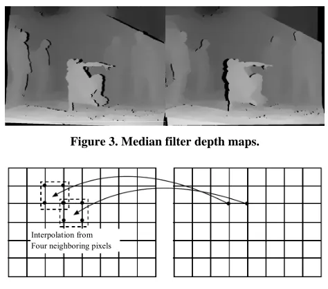
[image:3.595.304.541.517.726.2]In this step, the textures are retrieved by performing in-
Figure 3. Median filter depth maps.
Interpolation from Four neighboring pixels
Figure 2. The projected depth maps from two reference ca-
[image:3.595.56.289.623.710.2]projected point 2w onto multiple source image
planes, covering all regions of video scene.
[image:4.595.333.537.443.499.2] [image:4.595.56.288.634.721.2]3D P
Figure 5 shows the retrieved color images by inverse
warping using depth maps in Figure 3.
2.4. Pixel Classification and Initial New View Creation
Formally, suppose that we have a set of N texture im-
ages I
I I1, , ,2 IN
and depth images N
1, 2, , N
Z Z Z Z . Let Im
p and Zm
ph
be the
color and depth value at position of m t image.
In this step, we describe the type of pixels in the
syn-thetic view. We go through each pixel of all
input images and classify as stable, unstable and disoc-cluded pixels. To detect the types of pixel, we set the thresholds (depth threshold
pP N
Z
t and color threshold )
and examine the color and depth values for pixel C
t pP.
For each color channel, the color threshold C is set to
be 15 in our case. Depth threshold is the brightness in the depth map. In our experiments,
t
Z
t is set to 5 for the 8
bits depth quantization. A pixel is classified as:
If the depth value of a pixel at all input
depth images is less than depth threshold
pP N
Z
t , we classify
the pixel p as the disoccluded pixel. The color and depth
values of the pixel at synthetic view are set
tempo-rally to zero.
p
new 0, new 0 if k Z 1 2 , .
I p Z p , Z p t , k ,, N
(10)
If the depth value of a pixel at only one input
image is higher than the depth threshold and at all
remaining images is less than , we classify
P p Z t ) 1
(N tZ
the pixel p as the stable pixel. This is case the pixel p is
visible in only one view. The values of the pixel p at
synthetic view are just copied from the values of the pix-el p in the visible view.
, ,
if , , 1, 2, , , .
new k new k
k Z m Z
I p I p Z p Z p
Z p t Z p t m N m k
(11)
If the depth value of a pixel pP is higher than
Figure 5. Obtained color images by inverse warping.
the depth threshold tZ in more than one view, we
ex-amine both the color and depth values of the pixel to
detect the types of pixel.
p
First step, for each view , , we ex-
amine pixel . If the depth value of the pixel is higher than the depth threshold
k k1, 2, , N
p p
Z
t , then we check other
views j, j1, 2, , N, . If the view has
both a depth value of the pixel higher than the depth
threshold
jk j
p Z
t and has color similarity at p of view j
and k, Ij
p and Ik
p are called consistent color(the color similarity at pixel of two input images
and is defined based on the absolute color differences
p j
k
between Ij
p and Ik
p of , andchannels,
R G B
j k C
I p I p t
j j 1, 2, ,
). We count the total
number of view , N
k
having the consistent
color with view
k1, 2, , ,N jk
2,
k
at pixel p.
Assuming that for each view , this total
number is .
1, ,N
k
S
Second step, we find the biggest number of ,
as-suming that the biggest number is k
S M .
If M N 2 0.5 , we classify the pixel as the
stable pixel. Otherwise, the pixel is classified as the
unstable pixel. The value of unstable pixel can set to be
−1 so that they can be easily identified.
p p
The color and depth values of stable pixel at syn-
thetic view are rendered by blending
p
M pixels as fol-
lowing weighted interpolation:
new new 1 1 1 1 , M Mi i i
i i
M M
i i i
i i
I p w I p w z p
w z p w
(12)
where, wi is the weight factor assigned to view i,
i
I p and Zi
p are color value and depth value ofpixel at view i. The weight assigned to each view
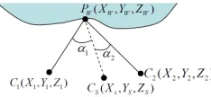
should reflect its proximity with the view being synthe- sized. The views that are closer to the synthetic view should have a bigger weight. In general, case, the weight
p
i
w can be set based on baseline spacing. However, for
more precise weighting, we use the angle distance deter-
mined by the point in 3D and camera positions as
shown in Figure 6. The weight factor wi is calculated
by
e if π 2
0 otherwis i ca i i a w
e (13)
where, is view index, i i is the angular distance of
view I and i is weight for the view at that pixel.
The constant controls the fall off as the angular dis-
w c
Figure 6. Weighted interpolation based on angular dis-tances.
minated as they view the scene the other side. In practice, has been found to work well.
1or 2
c
The new view is specified by
new new
1 2 1 2
,
InitialView , , , N , , , , N ,
I Z
I I I Z Z Z
N
(14)
where, is the procedure of pixel classifica-
tion and initial new view creation as above described.
InitialView
2.5. Find the Best Candidate for Unstable Pixel by Graph Cuts
In this step, we focus on refining initial synthetic view with unstable pixels. Unstable pixels have multiple pixel candidates and we want to predict the best candidate that minimizes the energy function described in following part.
We denote L as labeling space with
1, 2, ,L
U
, representing the image index and let
be the set of unstable pixels. Let fp be the label of
unstable pixel p and fpL. A labeling is to
as-sign a particular label
f
p
f to a pixel pU. With this
definition, our problem is to find the labeling f* to fill
the unstable region, such that the labeling f* has
min-imum cost.
We define our energy function based on the Markov Random Fields (MRF) formulation:
, ,
,
p p p q
p U p q N
E f D f V f f
p q (15)where, f is the labeling field, is the set of unsta-
ble pixels, and is the pixel’s neighborhood system.
U N
p p
D f is called the data term, which defines the cost
of assigning label fp to pixel . p Vp q,
fp,fq
de-notes the smoothness term that evaluates the cost of dis-
agreement between and which is assigned with p q
p
f and fq respectively. is a parameter to weigh
the importance of these two terms.
Data term Dp
fp is defined by
new
1
1
p p
p
p
p p f q f
q N N
f i
i
D f Z p O I p I q
I p I p
(16)where Np is neighboring pixels of p, Zfp
p is thedepth value of pixel p at candidate fp, Inew
q and(0 or 1) are the color value and disoccluded indicator
q
O
of pixel , respectively. q and are weight fac-
tors. Ii
p is color value of pixel p at input image . i
i j
I p I q represents the sum of absolute color
differences between Ii
p and Ij
q
of R, G and Bchannels.
The first part of data term enforces the candidate pixel selected to agree with its neighbor pixels. In addition, the neighboring pixel that is disocclusion does not influence the candidate selection process. It is also penalized less cost for the selecting a candidate pixel which has smaller
depth value Z because the pixel with smallest depth
value is closer to the camera and more likely defined the
color of synthetic pixel 2.
The second part of (16) is stationary cost, which de-fined based on color similarity at pixel p of all the input images. If the pixel has similar color at more input images, the stationary cost is smaller.
p
p
Smoothness term Vp q,
fp,fq
: measures the penaltyof two neighboring pixel and with different la-bels and is defined as follow:
p q
, ,
2
p q p q
f f f f
p q p q
I p I p I q I q
V f f
(17)
where, denotes the Euclidean distance in RGB color
spaces. The smoothness term gives a higher cost if fp
and fq do not match well. By incorporating such the
smoothness term, we can achieve visually smooth in the synthetic image.
We apply graph cuts optimization that is public avail-
able in [9] to minimize our energy function E f
.More detail about energy minimization with graph cuts can be found in [10,11].
This step is specified by
new new with
arg min ,
*
*
f f
f
I U I Z U Z f
E f
, ,
(18)
The refinement of image in Figure 7 by using graph
cut to select the best candidate for unstable pixel is
shown in Figure 8.
2.6. Inpainting Disocclusion Pixels Based on the Depth and Color Values of Neighboring Pixels
Figure 7. Initial synthesized view with 3 types of pixels. (The white color pixels are unstable pixels, the red color pixels are disoccluded pixels and the remaining pixels are stable pixels).
Figure 8. Refinement of initial synthesized image (image in Figure 7) by using graph cut (the red color pixels are disoc-cluded pixels).
inpainting method proposed by Tela [6]. Inpainting is a process of reconstructing lost or corrupted parts of im- ages using the values of neighborhood pixels. Although, these algorithms work sufficiently well, the resulting inpainted regions contain a notable blur because of the mixture background and foreground colors at the edge of disoccluded regions. In this paper, we develop a tech- nique based on inpainting method with depth information. We assume that the disoccluded pixels belong only to background, and we employ depth information to select accurately background pixels at the edges of disoccluded regions so that the blur can be avoided. Our method con-sists of several steps as follow.
First, for reducing processing time we find the small disoccluded regions by defining a window with the size
of centered at and counting the unstable pixel
inside this window. If the number of visible pixels
3 3 p
M
inside this window is higher than 50%, then the disoc- cluded pixels is inpainted by a weighted interpolation from visible pixels, which is specified by
1 1
new
1 1
1 1
new occ
1 1
,
, ,
M M
occ i new i i
i i
M M
occ i new i i
i i
I p d I p d
Z p d Z p d p
O
(19)
where, M is number of visible pixels inside the
win-dow. O is disoccluded region, and i is distance from
disoccluded pixel to visible pixel .
d
occ
p pi Inew
piand Znew
pi are color and depth values of the visiblepixel i.
Second, for each pixel o in remaining disoccluded
regions we search in eight directions to find the pixel u,
which has the smallest depth value
p
p
p
min
Z at the edge of
disoccluded region and the distance u from this point
to . We define a window with the size of
d
o
p
du
du
centered at po (at first, 0),and we count the visible pixels which have depth value
Z with ZZmin 5. If there are not enough 50% of
visible pixels inside the window, we increase the size of
window by increasing . Finally, disoccluded pixels are
inpainted by a weighted interpolation from visible pixels according to (19).
With inpainting procedure describing above, this step can summarized by
, Inpaint ,
final final new new
I Z I
Z . (20)
3. Experimental Results
We quantify the proposal method performance based on
Peak Signal Noise Ratio ( ) and the structural simi-
larity (SSIM) index between a reference image r and a
synthetic image s. SSIM index is a method for meas-
uring the similarity between two images [12]. The SSIM index value 1 is only reachable when two images are identical and the higher PSNR normally indicates that it is higher quality synthetic image. Before computing
, the images are converted from RGB color space to YUV color space, and Y channel is used for calcula-tion. Y channel is defined by
PSNR
I I
PSNR
). , ( 114 . 0 ) , ( 587 . 0 ) , ( 299 . 0 ) ,
(i j Ri j G i j B i j
Y (21)
The PSNR can be calculated by
), ) , ( ) , ( 1
255 (
log
10 1, 1
0 , 0
2 2
10
w h
j i
s r i j Y i j Y
h w
PSNR (22)
where, and h are the image width and height. r
and s are the channels of reference image and syn-
thetic image, respectively.
w Y
Y
ated and distribution by Interactive Visual Group at Mi- crosoft Research [13]. These datasets include a sequence
of 100 images of 102 pixels captured from 8
cameras with the calibration parameters. Figure 9 shows
the camera arrangement of these two sequences. Depth maps for each view are also provided. For more detail about these depth maps generation, please refer to [2].
4 768
In our paper, the synthetic view is set to be the same as the actual camera. View 3 and 5 are used with depth
maps to synthesize view 4. Figure 10 shows the example
[image:7.595.337.508.88.650.2]of view synthesis results. The experimental results show that the proposed method achieved on average over 34 dB in PSNR and 0.93 index value in SSIM on the two sequence “Break-dancer “and “Ballet”.
Figure 11 shows our PSNR and SSIM comparison
with those of Sohl et al. [14] over 100 frames for the
“Break-dancer” and “Ballet” sequences.
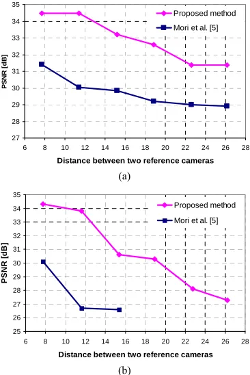
Because usually the number of cameras is limited, the camera arrangement is very importance for obtaining a
good quality of synthesized view. Figure 12 shows our
quality of synthesis with varying the distance between the two reference cameras comparing the method
[image:7.595.57.286.376.448.2]pre-sented by Mori et al. in [5], where our measurements
Figure 9. A configuration of “Break-dancer” and “Ballet” sequences with 8 cameras [2].
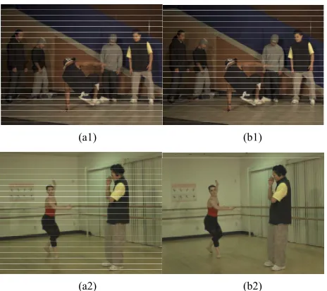
(a1) (b1)
(a2) (b2)
Figure 10. Example of the synthetic view. (a1) Original view image; (b1) Synthesized image (PSNR = 34.7 dB; SSIM = 0.94); (a2) Original view image; (b2) Synthesized image (PSNR = 34.6 dB; SSIM = 0.95).
30 30.5 31 31.5 32 32.5 33 33.5 34 34.5 35 35.5
0 10 20 30 40 50 60 70 80 90
Frame Index
P
S
NR (
d
B) Sohl et al. [14]
Proposed method
(a)
0.6 0.65 0.7 0.75 0.8 0.85 0.9 0.95 1
0 10 20 30 40 50 60 70 80 90
Frame Index
SSI
M
Sohl et al. [14] Proposed method
(b)
30 30.5 31 31.5 32 32.5 33 33.5 34 34.5 35
0 10 20 30 40 50 60 70 80 90
Frame Index
PS
NR (
d
B) Sohl et al. [14] Proposed method
(c)
0.6 0.65 0.7 0.75 0.8 0.85 0.9 0.95 1
0 10 20 30 40 50 60 70 80 90
Frame Index
SSI
M Sohl et al. [14]
Proposed method
[image:7.595.57.289.482.688.2](d)
Figure 11. PSNR and SSIM comparison: (a) PSNR for “Break-dancer”, (b) SSIM for “Break-dancer”, (c) PSNR for “Ballet”, (d) SSIM for “Ballet”.
correspond to an average over 100 frames.
The measured synthetic qualities are compared with
27 28 29 30 31 32 33 34 35
6 8 10 12 14 16 18 20 22 24 26 28
Distance between two reference cameras
P
S
NR [
d
B]
Proposed method Mori et al. [5]
(a)
25 26 27 28 29 30 31 32 33 34 35
6 8 10 12 14 16 18 20 22 24 26 28
Distance between two reference cameras
PS
N
R
[
d
B
]
Proposed method Mori et al. [5]
[image:8.595.81.264.85.359.2](b)
Figure 12. PSNR versus distance between camera for (a) “Break-dancer” sequence, (b) “Ballet” sequence.
Table 1. Exerimental results comparision.
Method “Break-dancer” “Ballet”
PSNR (dB) SSIM PSNR (dB) SSIM
Sohl et al. [14] 30.8 0.68 30.7 0.66
Mori et al. [5] 31.4 Reported Not 30.1 Not Reported
Proposed method 34.5 0.93 34.3 0.94
results, the average PSNR of proposal is superior to that
of other methods such as Mori et al. [5], Sohl et al. [14]
with a gain of 3.0 dB. The structure similarity (SSIM) of
our method is higher than that of Sohl et al. method.
Moreover, in multi-view configuration, we have cameras, which capture the scene at difference positions. For our experimental case, there are 8 cameras. Thus, instead of using only two neighbor views as above con-ventional methods, we can use more than two images to synthesize a new view. Our proposal can do this idea easily. Our experiment shows that using four reference views (two views on both left side and right side) to syn-thesis a new view, a higher PSNR (about 0.5 - 1 dB) and SSIM are obtained than the case of using two reference views.
N
4. Conclusions
In this paper, we propose a novel synthesis method that
enables to render a free-viewpoint from multiple existing cameras. The proposed method solves the main problems of depth based synthesis by performing the pixel classi- fication to generate an initial new view from stable pixels and using Graph cuts to select the best candidate for un- stable pixels. By defining the types of pixels and using Graph cuts, the color is consistent and the pixels are wrapped incorrectly because inaccuracy depth maps are removed. The remained disoccluded pixels are inpainted by using depth and texture neighboring pixel values. Considering depth information for inpainting, blurring between foreground and background textures are reduced. Experimental results show that the proposed method has strength in artifact reduction. In addition, our smooth term makes the result visually smooth. Objective evalua- tion has shown that our method gets a significant gain in PSNR and SSIM comparing to some other existing methods. Another advantage of our method is that we can use a set of un-rectified images in multi-view system to create a new view with higher quality.
The drawback of our method is using Graph Cuts, which is time consuming. However, we just only apply Graph Cuts for unstable pixels, which are a small amount of pixels comparing to the whole image, so the time for Graph Cuts can be reduced.
The future work will focus on more improving synthe- sis quality with utilizing temporal information in succes- sive video frames.
5. Acknowledgements
We would like to thank Interactive Visual Media Group, Microsoft Research for distributing multi-camera video data and the anonymous reviewers for their comments.
REFERENCES
[1] M. Tanimoto, “Overview of FTV (Free-Viewpoint Tele- vision),” Proceedings of the 2009 IEEE International Conference on Multimedia and Expo, New York, 28 June-3 July 2009, pp. 1552-1553.
doi:10.1109/ICME.2009.5202803
[2] C. L. Zitnick, S. B. Kang, M. Uyttendaele, S. Winder and R. Szeliski, “High-Quality Video View Interpolation Us- ing a Layered Representation,” ACM Transactions on Graphics, Vol. 23, No. 3, 2004, pp. 600-608.
doi:10.1145/1015706.1015766
[3] K. Pulli, M. Cohen, T. Duchamp, H. Hoppe, L. G. Shapiro and W. Stuetzle, “View-Base Rendering: Visual- izing Real Objects from Scanned Range and Color Data,” Proceedings of the Eurographics Workshop on Rendering Techniques‘97, St. Etienne, 16-18 June 1997, pp. 23-24. [4] K. Muller, K. Dix, P. Merkle, P. Kauff and T. Wiegand,
[image:8.595.58.285.415.503.2](ICIP), San Diego, 12-15 October 2008, pp. 2448-2451 [5] Y. Mori, N. Fukushima, T. Yendo, T. Fujii and M. Tani-
moto, “View Generation with 3D Warping Using Depth Information for FTV,” Signal Processing-Image Commu-nication, Vol. 24, No. 1-2, 2009, pp. 65-72.
doi:10.1016/j.image.2008.10.013
[6] A. C. Telea, “An Image Inpainting Technique Based on the Fast Marching Method,” Journal of Graphics Tools, Vol. 9, No. 1, 2004, pp. 25-36.
doi:10.1080/10867651.2004.10487596
[7] S. Zinger, L. Do and P. H. N. de With, “Free-Viewpoint Depth Image Based Rendering,” Journal of Visual Com- munication and Image Representation, Vol. 21, No. 5-6, 2010, pp. 533-541.doi:10.1016/j.jvcir.2010.01.004 [8] K.-J. Oh, S. Yea and Y.-S. Ho, “Hole Filling Method
Using Depth Based In-Painting for View Synthesis in Free Viewpoint Television and 3-D Video,” Picture Cod-ing Symposium, Chicago, 6-8 May 2009, pp. 1-4.
[9] V. Kolmogorov and R. Zabih, “What Energy Functions Can Be Minimizedvia Graph Cuts?” IEEE Transactions on Pattern Analysis and Machine Intelligence, Vol. 26, No. 2, 2004, pp. 147-159.
doi:10.1109/TPAMI.2004.1262177
[10] Y. Boykov, O. Veksler and R. Zabih, “Fast Approximate
Energy Minimization via Graph Cuts,” IEEE Transac-tions on Pattern Analysis and Machine Intelligence, Vol. 23, No. 11, 2001, pp. 1222-1239.
doi:10.1109/34.969114
[11] Y. Boykov and V. Kolmogorov, “An Experimental Comparison of Min-Cut/Max-Flow Algorithms for En- ergy Minimization in Vision,” IEEE Transactions on Pattern Analysis and Machine Intelligence, Vol. 26, No. 9, 2004, pp. 1124-1137.doi:10.1109/TPAMI.2004.60 [12] Z. Wang, A. C. Bovik and H. R. Sheikh, “Image Quality
Assessment: From Error Measurement to Structural Sim- ilarity,” IEEE Transactions on Image Processing, Vol. 13, No. 4, 2004, pp. 600-612.doi:10.1109/TIP.2003.819861 [13] S. M. Rhee, Y. J. Yoon, I. K. Shin, Y. G. Kim, Y. J. Choi
and S. M. Choi, “Stereo Image Synthesis by View Morphing with Stereo Consistency,” Applied Mathemat-ics & Information Sciences, Vol. 6, 2012, pp. 195-200. [14] M. Solh and G. AlRegib, “Hierarchical Hole-Filling for
Depth-Based View Synthesis in FTV and 3D Video,” IEEE Journal of Selected Topics in Signal Processing, Vol. 6, No. 5, 2012, pp. 495-504.