5080
SIMULATION OF CHAOTIC PHENOMENA IN
INFOCOMMUNICATION SYSTEMS WITH THE TCP
PROTOCOL
1ALEXAND KARPUKHIN, 1DMITRIJ GRICIV, 2EVGENY NIKULCHEV,
1Kharkov National University of Radio Electronics, Kharkiv, Ukraine
2MIREA – Russian Technological University, Moscow, Russia
E-mail: 1[email protected], 2[email protected]
ABSTRACT
In numerous works devoted to the study of network traffic, it was shown that in high-speed networks, chaotic operation modes can appear, the main cause of which is the behavior of the TCP protocol. The presence of such modes leads to a significant reduction in the bandwidth of the entire network, especially in the so-called bottlenecks. However, models that adequately describe infocommunication systems and make it possible to apply the entire arsenal of classical methods for analyzing nonlinear dynamical systems have not been proposed yet. The paper proposes a new approach to the analysis of the behavior of infocommunication systems with the TCP protocol – treating them as nonlinear dynamical systems demonstrating chaotic properties for certain values of the parameters. Phase portraits of the considered systems are constructed; the values of the maximum Lyapunov exponent are calculated for different values of the main parameters of the systems. The physical experiment was carried out in the real network. The problem of optimizing the parameters of the infocommunication system was solved in terms of the absence of undesirable chaotic regimes.
Keywords: Network Traffic, TCP Protocol, Lyapunov Exponent
1. INTRODUCTION
Two-way information flow between a pair of adjacent systems in the network provides a channel connecting two systems. The main characteristics of the channels are the rate of the information flow (bandwidth) and the delay in transmission. At each point of connection of the router to the channel there is a buffer in which the queue of data expected to be sent via this channel is organized. The buffer capacity and bandwidth are the shared resources of the network. If the speed of access to the router exceeds its maximum possible output speed, then the network is overloaded, which results in buffer overflow and loss of information (packets). Overloading the network leads to the formation of the so-called congestions in some parts of the network, called bottlenecks. The main parameters that determine the behavior of the TCP connections in narrow places are bandwidth, delay in the channel and the buffer size of the router.
The transport layer protocol takes the most important position in any network architecture, including TCP / IP, because it provides reliable and efficient transmission of information (in the form of
packets) directly between the end systems of the network. For this purpose, the transport protocol specifies an agreed set of rules of conduct for the participants in the information exchange. These rules regulate the joint access of nodes to the shared resources of the network, so the effectiveness of the transport protocol determines the efficiency of the entire network as a whole.
5081 There is a send window (swnd) on the sending packets host, and there is a receive window (rwnd) on the accepting packets host [1–3].
TCP monitors the data flow. Each side of the TCP connection has a specific buffer space. TCP on the receiving side allows the remote side to send data only if the recipient can place them in the buffer. This prevents slow hosts from overflowing caused by fast hosts.
When working with a slow start, another window is added to the sending TCP: an overflow window called congestion window (cwnd). When a new connection is established with a host located on another network, the size of the overflow window is set equal to the size of one segment (the segment size is declared by the remote end). Each time an ACK is received, the overflow window is incremented by one segment. The sender can transfer the amount of data up to the minimum size of the overflow window and the advertised window. With the overflow window, the sender manages the flow, while the receiver uses the advertised window to control the flow.
At a certain point, the maximum transmission for a given connection (the joint network) is reached, in which case the intermediate router begins to drop packets. This indicates that the size of the sender's overflow window has become too large.
The article gives an overview of the authors' work in the field of modeling infocommunication networks with the TCP protocol, containing a new methodology for studying such systems. In particular, a new approach to the modeling of computer networks with the TCP protocol is proposed. Several TCP-compounds coexisting in the same channel are represented as an ensemble of
nonlinear mathematical pendulums. A
mathematical model of a set of TCP connections in one physical channel in the form of an ensemble of coupled nonlinear oscillatory systems is developed. A method for analyzing the behavior of several neighboring TCP connections using phase portraits and the Lyapunov exponent is developed, which makes it possible to investigate chaotic regimes of computer networks. A method for analyzing the behavior of computer networks in the presence of overloads is developed.
2. ANALYSIS OF LITERARY SOURCES
The emergence and widespread use of computer networks, as well as the increase in the number of diverse network services (WWW, IPhone, etc.) has led to the fact that network traffic has become more complex and unpredictable.
These properties became especially developed with the advent of high-speed data transmission technologies. This is due to the fact that one of the main performance indicators (QoS) of packet-based networks is the number of lost packets. The loss (drop) of packets in cases of inability to process them due to the buffer overflow of the router leads to additional load on the network (packets remain on the network and are sent again in the absence of ACK) and, ultimately, to congestions. Packet data loss rates, expressed in fractions of a percent, lead to significant information losses.
In the last 10-15 years, a large number of works have been devoted to the investigation of network traffic. They can be divided into two groups. The first (and the most extensive) includes works in which the authors analyze network traffic and determine its statistical characteristics, in particular the Hurst indicator, which characterizes the degree of self-similarity of traffic.
The application of the concept of self-similarity to telecommunication systems was first proposed by Mandelbrot [4]. The main reason for the emergence of chaotic phenomena, according to many researchers, is the behavior of the main transport protocol Internet-TCP [5, 6].
The source of the analyzed data is either a full-scale experiment (for example, [7]) or modeling by software (for example, ns [8], OPNET [9]). The modeling methods are the construction of a regression model [10] or combination of regression model and fuzzy system [11], or use Haar transform [12] or neural networks [13] ets.
The second group includes works, in which the authors regard the infocommunication system as a dynamic system in which self-similarity is an internal property of the system itself [14]. In [14], the authors used the method of reconstructing multi-dimensional trajectories of a dynamical system [15], which consists in using time-shifted samples of congestion window values for two TCP connections when using a network simulator ns-2 [16]. The phase portraits constructed in [14], as well as the calculated values of the maximum Lyapunov exponent for the dynamical system under study, convincingly prove the existence of chaotic regimes for certain values of the system parameters. The method of multidimensional phase space is most widely used for constructing mathematical models [17, 18]. However, this method has drawbacks that limit the scope of its application:
5082 • the assumption that the coordinates can be considered independent is often too rough;
• the application of this method causes certain difficulties when it is necessary to take into account the different times of interaction of the subsystems.
Difficulties in identifying real functioning systems determine the most widely-oriented approach to modeling non-linear objects, which consists in choosing the kind of mathematical model in the form of an evolutionary equation and subsequent identification of parameters, or nonparametric identification of the model. The model is considered adequate if the evaluation of the given adequacy criterion, calculated as the dependence of the model residual on the experimental data, is within the permissible limits.
Especially relevant researches in the field of traffic modeling in infocommunication networks has become in recent years due to the rapid development, first of all, of new services on the Internet (VoIP, etc.), as well as intensive use of the Internet in such areas as GRID [19] and Cloud Computing [20]. This is also important in such areas as high-performance computing in parallel and distributed systems [21].
In the works of many authors it is noted that aggregated network traffic is self-similar [22]. It is shown that the variance-gamma distribution of file sizes, the appearance of packets, and the duration of transmission make a major contribution to the self-similar nature of aggregated network traffic.
Various methods are used to analyze network traffic. One of the parameters, by which the degree of self-similarity is determined, is known to be the Hurst parameter.
It is also obvious that TCP itself is the primary cause of self-similarity and its behavior can have undesirable consequences in infocommunication networks with the increase in the capacity of global computer networks (WAN) to values that are expressed in several gigabytes per second. In particular, even if the traffic generated by
applications has a Hurst parameter H = 0.5 (that is,
it is not self-similar), TCP "modulates" this traffic and makes it self-similar (having the Hurst parameter H = 1.0). Moreover, all the existing TCP (Reno, Vegas, Tahoe) implementations have this "undesirable" property, which is due to the presence in all protocol variations of the cwnd parameter controlling the number of packets entering the network and which varies in time according to a nonlinear law.
3. MODEL NETWORK
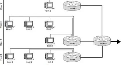
[image:3.612.314.524.401.515.2]To investigate the self-similarity of network traffic, a model TCP / IP network was created (Figure 1) in which all hosts are connected to the router by a point-to-point connection. The model network is a step structure of four floors, each of which hosts and a router were installed. This structure was chosen as one of the most often used for offices or multi-storey buildings. On all hosts the special software was installed, the so-called sniffer (wireshark), which captured incoming and outgoing network traffic and recorded data in real time. To connect hosts to routers (Cisco Catalyst 2960G-48), a twisted pair was used. Thus, the maximum throughput of this section of the network is Cb = 100Mbps. In turn, optical fiber was used to connect the routers to each other. As a result, the installed software created several dumps with data on one host. This was done in order to assess the load on the model network at different times of user activity. Time to capture network traffic on hosts was 11,000 seconds (about 3 hours), which, in our opinion, is sufficient for a comprehensive analysis of this part of the network. Saved reports with data were then transferred to a remote computer for further processing.
Figure 1. Model network topology
5083 MySQL, HTTP, NNTP, X11, NAPSTER, IRC, RIP, BGP, SOCKS 5, IMAP 4, VNC, LDAP, NFS, SNMP, MSN, YMSG, etc. Interception of traffic of the network interface is carried out in real time. It is also possible to filter captured packets by a variety of criteria and create a variety of statistics. Wireshark operates on the basis of the pcap library (Packet Capture), which allows analyzing the network data that comes to the network card of the computer. Interception of traffic by the analyzer provides the following options: interception of traffic of various types of network equipment (Ethernet, Token Ring, ATM and others). The termination of interception occurs on the basis of various events: the size of the intercepted data, the duration of interception, the number of intercepted packets. It supports the display of decoded packets during the interception and packet filtering in order to reduce the size of the intercepted information, as well as the recording of dumps into several files, if the interception continues for a long time.
4. TIME SERIES PROCESSING
TECHNIQUE
During the capture of traffic in the network, the value of many variables was monitored for each host, so the received data reports were filtered according to the following criteria: host IP address and TCP data transfer protocol.
For further analysis of time series, it was necessary to convert the original series
1 2
{ ( ), ( ), ..., ( )}t t tn
into equidistant ones,
which have a constant step t along the time axis.
This value t can be designated as the degree of
aggregation. To do this, a new series was generated, which was obtained by the operation of summing each initial information value (TCP traffic) in
accordance with a given time interval t. Thus,
the aggregated values of the pre-formed series can be represented in this form:
1 ( 1)
N t
N i
i N t
X t
, (1)As a result of the algorithm, an aggregated
equidistant traffic realization is obtained
{ ( ), (2 ), ..., ( )},
X X t X t X N t containing N
elements. The physical meaning of each of its elements is the total speed (byte / sec) on the
corresponding interval t. In the process of
aggregating time series, different time intervals
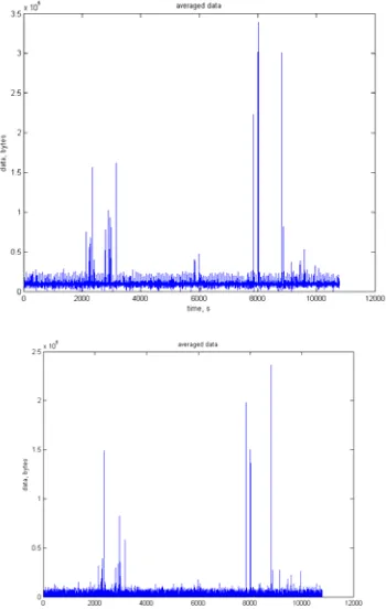
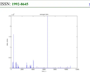
were selected t = 0.1, 0.5, 1, 2, 5, 10. Graphs 2
and 3 are shown below. They show the aggregated
traffic for the same aggregation level t 0.1 and
1
t
for various sessions of the model network
operation. It is noteworthy that the structures of the obtained series for any level of aggregation are similar in structure to each other.
[image:4.612.331.506.227.503.2]As you can see in Figures 2 and 3, the frequency of the TCP protocol is observed, so-called on / off modes in the model network. As expected, network traffic has an explosive nature at different time intervals. And also with a different aggregation step, the time series retains the invariance property.
5084
Figure 3. Aggregate time series (traffic) for host 3 at t
=0.1 and t=1
5. ANALYSIS OF CHAOTIC
CHARACTERISTICS
5.1. Fractal dimension and Hurst index
Fractals are structures that at different scales look approximately the same [24-26]. Multifractals are inhomogeneous fractal objects, for the full description of which, in contrast to regular fractals, it is not enough to introduce just one fractal dimension, but a spectrum of such dimensions is needed. The reason for this is that along with purely geometric characteristics, such fractals also possess some statistical properties.
The parameter H, 0H 1, called the Hurst
exponent, is the degree of self-similarity. Along
with this property, the indicator H characterizes
the measure of the long-term dependence of the stochastic process. This value decreases when the delay between two identical pairs of values in the time series increases.
Аor a self-similar process, local properties are reflected in global properties in accordance with the
well-known relationship D n 1 H between
fractal dimension D and the Hurst coefficient H
for a self-similar object in n-dimensional space. In our case, n = 1 for the time series, and, accordingly,
the fractal dimension D of the time series is
related to the exponent of its fractality (the Hurst
exponent) H by the formula H 2 D. Thus,
self-similarity parameters H and D are measures
of stability of a statistical phenomenon or a measure of the duration of a long-term dependence of a stochastic process.
Values H 0.5 or D1.5 indicate
independence (the absence of any memory of the past) of the increments of the time series. The series
is random, not fractal. The closer the value H to 1,
the higher the degree of stability in the long-term
relationship. The range 0H 0,5 corresponds to
antipersistent series: if the antipersistent series was characterized by growth in the previous period,
then the closer the Hurst index to 0, the more likely the decline in the next period will begin. For values
0.5H1, the series demonstrates persistent
(trend-resistant) behavior. If the persistent series increased (decreased) in the previous period, then the closer the Hurst index to 1, the more likely the behavior of this series will remain for the same period in the future.
5.2. The method of multifractal detrended fluctuation analysis
When estimating the parameter H for
self-similar time series, the detrended fluctuation analysis (DFA) method is used [27, 28]. In this
case, for the initial time series x t( ), a cumulative
series is constructed y t( )
ti1x t( ), which isdivided into N segments of length
s
. For eachsegment y t( ), the fluctuation function is calculated
1
22
1 1
m t
F s y t Y t
s
, (2)where Y tm( ) is the local
m
-polynomial trendwithin a given segment.
The function F s( ) is averaged over the entire
series y t( ). Such calculations are repeated for
different sizes of segments to obtain a dependence
( )
F s over a wide range of parameter s values.
For processes with fractal properties
s
, thefunction F s( ) also increases with increasing, and
the linear dependence log ( )F s on logs indicates
the existence of the scale invariance property:
HF s s . (3) When studying the properties of multifractal processes, multifractal detrended fluctuation analysis (MFDFA) is used [29]. When the MFDFA is carried out, the dependence of the fluctuation
function F sq( ) on the parameter q is
investigated:
1
2 2
1
1 N q q
q
i
F s F s
N
, (4)obtained by raising the expression (12) to a power
q and then averaging over all segments.
Changing the time scale
s
for a fixed indexq, we find the dependence F sq( ), representing it
in double logarithmic coordinates. If the series under investigation is reduced to a multifractal set, exhibiting long-term dependences, then the
fluctuation function F sq( ) is represented by a
5085
h(q)F s s , (5) with the function of the generalized Hurst exponent
( )
h q . From the definitions (2) and (4) it follows
that with q2 this index is reduced to a normal
value H.
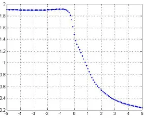
In the presented work, the multifractal characteristics of the aggregated data traffic were investigated. The estimation of the generalized Hurst index for realizations of aggregated traffic for several hosts of the model network under consideration with the same level of aggregation
0.1
t
[image:6.612.119.271.252.375.2] is shown in Figures 4 and 5.
[image:6.612.122.269.431.551.2]Figure 4. Function h q( ) for realizations of time series for host 2, H = 0.62
Figure 5. Function h q( ) for realizing the time series for host 3, H = 0.55
The analysis showed that the analyzed traffic realizations have clearly expressed multifractal properties: the range of the generalized Hurst index
is 1.5 h 4, and the multifractal structure of the
series varies significantly depending on the choice of a host. The Hurst index H in almost all cases exceeds 0.5, which indicates the long-term dependence of the studied series.
The maximum Lyapunov exponent
Having an aggregated time series, it is possible to calculate the Maximum Lyapunov Exponent (MLE) – a value that characterizes the rate of divergence of close trajectories, the positive value of which is usually taken as an indicator of the chaotic behavior of the system. The calculation of the maximum Lyapunov exponent was carried out with the help of the TISEAN package [30], which is intended for the analysis of time series and is based on the theory of nonlinear deterministic dynamical systems or chaos theory [31]. TISEAN represents the implementation of a number of
algorithms of chaos theory. In this case, the lyap_k
utility from the TISEAN package was used to calculate the maximum Lyapunov exponent. The result of its work is a set of data representing the dependence of the logarithm of the trajectory runoff
coefficient on time S
, ,m n
, which is calculatedas follows:
0
0 1 0 0
, ,
1 ln 1
( ) n n
N
n n n n
n n S U S
S m n
S S N U S
,(6)where
is the neighborhood of the point Sn0,m
is the dimension of the phase space, n is the
time, and U S( n0) is the neighborhood of the point
0 n
S of diameter
.If the value S
, ,m n
exhibits linear growth with the same slope in a reasonable range of values, then the tangent of the slope of the straight line
approximating this section can be assumed to be approximately equal to the maximum Lyapunov exponent.
[image:6.612.318.516.517.670.2]5086
Figure 7. Calculation of the Lyapunov exponent of host 3 at Δt = 0.1, λ ~ 0.188
As seen from the graphs, MLE > 0, this indicates that the system in question shows chaotic behavior. A comparative analysis was also carried out between the maximum Lyapunov exponent and the aggregation level of time series to assess how these two parameters correlate. With a reasonable change in the step of aggregation of the time series, the value of the maximum Lyapunov exponent practically did not change.
5.3. How relevant is the work in this direction
This work is relevant because chaotic phenomena, observed in infocommunication networks with certain values of their parameters, lead to a significant reduction in the capacity of networks. Therefore, the determination of the values of the parameters of infocommunication networks, in which unwanted chaotic phenomena arise (or do not arise) will enable to design (and accompany during their life cycle) autonomous telecommunication systems with the TCP protocol, in which there will be no chaotic phenomena, which will lead to an increase in their throughput ability.
6. MATHEMATICAL MODELING OF THE
BEHAVIOR OF TCP CONNECTIONS 6.1. Test stand
In this paper, a discrete-time simulator with open source code ns-3 (Network Simulator 3) was used to study the behavior of TCP streams. It provides the researcher with a set of classes, using which, inheriting and modifying them; it is possible to model a wide range of protocols and processes occurring in computer networks. Also, the simulator allows you to simulate real-time processes and integrate it with a testbed, make a testbed part of the simulated network, etc. [32]. The simulator ns-3 contains a set of tests for all
components, which guarantees the reliability of the results obtained.
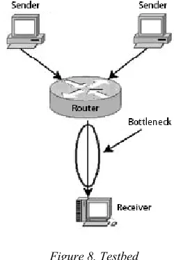
Using this simulator, a TCP / IP network model was created (see Fig. 8), where all the host computers are connected to the router by a point-to-point connection. The sending hosts simulated the work of applications sending data at a constant bitrate to the destination host, where an application that received data from both hosts was running. The
speed of data generation by senders (Cf), delay
(db), and bandwidth (Cb) of channels in a
bottleneck, as well as the delay (d) and the bandwidth (C) of channels for sending hosts could be varied by setting parameters for each new numerical experiment. Another changed parameter
was the size of the Drop Tail Queue (Qs) data
queue on the network interface of the router connected to the receiver. The receiving host window (rwnd) was intentionally made very large, so that only the value of the overload window (cwnd) was the limiting factor.
Figure 8. Testbed
Obviously, the state of congestion in such a network will arise when the total rate at which host senders send data will exceed the capacity of the receiver's channel. Moreover, the key parameters
influencing the occurrence of overload will be Cf,
b
d , Cb, and Qs, since with sufficient bandwidth of
the hosts-senders’ channels and a small delay, they will not influence the TCP congestion control algorithm. In the future, when describing numerical experiments, only these parameters will be given.
6.2. Methodology for studying the behavior of the TCP protocol.
[image:7.612.350.475.347.533.2]5087 number in the real dynamic system under investigation). But it is possible to choose the corresponding section of the phase space by a proper choice of these phase variables. The value of
the overload window (cwnd) was selected, since it
directly affects the data transfer rate.
During the simulation of the operation of two
TCP connections, the cwnd values of each TCP
stream were tracked from senders to the recipient. As a result, two time series were obtained (for two hosts), which set the step function of the cwnd dependence on time.
It was proposed in [15] to use the time series
2
[ ,x xt tt,xt t,...] averaged over N as an easily measurable characteristic of complex systems and it was shown that it can be used to reconstruct hidden multidimensional trajectories. This method, applied
to the values of the overload window (cwnd), leads
to the relations [8]:
1
1
1
[ ] [ ],
1
[ ] [ ].
N
x j
N
y j
x i cwnd i j N
y i cwnd i j N
, (7)Here, x and y denote two TCP streams. The
value of N is responsible for the averaging scale
and is larger than N, the more hidden dimensions of the system can be recovered.
In this case, the functions cwnd(t) are different
for each of the hosts and only the moments of changing the value of this functions are fixed. Therefore, in order to apply the above-described method and construct a phase portrait, it is necessary to take the values of the overload window at the same time points.
6.3. Phase portrait
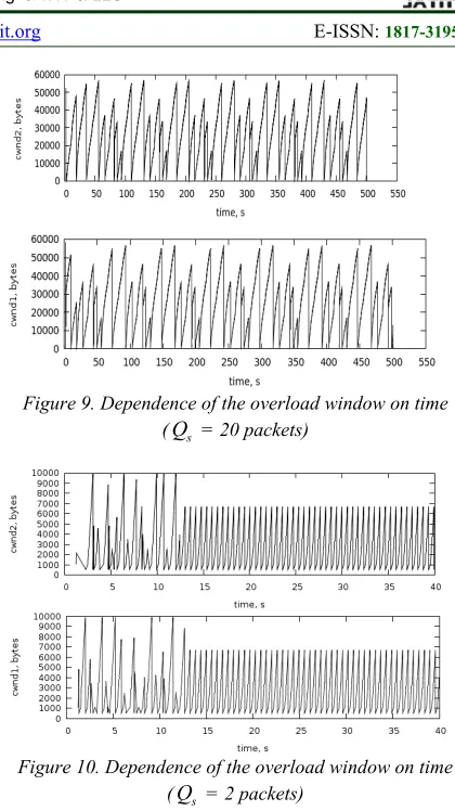
At certain parameters of the test bench, the test system under discussion shows rather complicated behavior. In particular, below are
graphs of the dependence of cwnd(t) at Cf = 5
MB/s, db = 10 ms, Cb = 5 MB / s, Qs = 20 packets
(1 packet = 536 bytes, in all the numerical
experiments) (Fig. 9) and harsh mode for Qs = 2
packets (Fig. 10). On both time-series graphs, one can observe the presence of a regular "beat", i.e. each of the TCP streams alternately takes advantage of each other for a certain amount of time in an attempt to capture the available bandwidth of the channel.
Figure 9. Dependence of the overload window on time (Qs = 20 packets)
Figure 10. Dependence of the overload window on time (Qs = 2 packets)
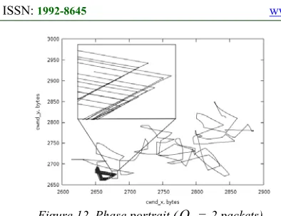
The phase portraits corresponding to Fig. 9 and 10, obtained by processing the data, according to the algorithm described in the previous section,
at N = 2000 and t = 10ms are shown in Fig. 11
[image:8.612.309.519.64.438.2]and Fig. 12.
5088
Figure 12. Phase portrait (Qs = 2 packets)
As can be seen, the phase trajectories form the limit cycle, which has a rather fine structure. Moreover, this trajectory is fairly stable: when the time of the start of TCP flows changes relative to each other, the depicting point after a small "wander" begins to describe the same closed trajectory.
If there is no overload (Qs = 100 packets), the
cwnd value of both hosts grows unlimited, and there are no anomalies on the phase portrait.
6.4. The maximum Lyapunov exponent.
The phase portraits are convenient in that they not only can visually display the state of the dynamic system, but also make it possible to calculate the maximum Lyapunov exponent λ, a value that characterizes the rate of divergence of close trajectories, the positive value of which is usually taken as an indicator of the chaotic behavior of the system. However, it is possible to build a phase portrait of the system only in a small number of cases. When one new sender is added to the simulated system, the dimension of the phase space under study will also increase by one, and it will be more difficult to analyze the obtained data, not to mention that visualization of the phase space is possible only if its dimension is less than 4.
Thus, you need a tool that will allow you to analyze the received data regardless of the number of available TCP sessions. For this purpose, a package of TISEAN utilities (intended for time series analysis [30, 31]) was chosen based on the theory of nonlinear deterministic dynamical systems or chaos theory.
Below are the results obtained after processing and visualization of the time series of cwnd(t), corresponding to Fig. 11 (see Figure 13), using the
lyap_k utility. The figure shows curves S( , , m n )
for five different values of ε and a straight line
y a bx approximating the linear portion of
these curves. Thus, the value of b is numerically equal to the maximum Lyapunov exponent. If there is no overload, the Lyapunov exponent λ < 0, and
[image:9.612.314.518.77.267.2]hence such a system does not exhibit chaotic behavior.
Figure 13. Calculation of the Lyapunov exponent
6.5. New mathematical approaches
The process of packet transmission in accordance with the TCP protocol can be represented as a vibrational process whose frequency is determined by the length of the spatial interval (or propagation time) between two points of the information signal. At the time the
information is transmitted, the ACK
acknowledgment delay time associated with the impact of one protocol on another is affected. The longer the delay time, the closer the behavior of the co-oscillatory process to the behavior of the physical pendulum near the separatrix. On the separatrix, the pendulum can be delayed for a fairly long time, which in the process under consideration is related to the waiting time for receipt in the conditions of competition of various independent protocols. Since the behavior of the pendulum near the separatrix has a nonlinear character, under conditions where the protocols influence each other, the interaction condition of nonlinear pendulums is considered. Thus, single protocols are described by mathematical pendulums, and when the protocols influence each other, the behavior of a nonlinear pendulum near the cessation of the separatrix is observed.
5089 interacts with neighboring TCP connections, which allows us to consider them as an ensemble of macroscopic nonlinear systems.
From the point of view of information transfer in each TCP connection, the following occurs: the sender transmits the segments formed to the receiver, and in response receives a segment receipt acknowledgment (so-called ACK). From a physical point of view, in the first approximation, this process can be represented as the oscillations of some mathematical pendulum. Thus, each TCP connection can be represented as a nonlinear oscillatory system.
A mathematical model of interacting TCP connections is proposed in the form of an ensemble of nonlinear mathematical pendulums in which each TCP connection acts as a pendulum [34-38].
In this case, n of the TCP connections can be
described by the following system of differential equations
'' 2
1 1 1 1 2 3
'' 2
2 2 2 2 1 3
'' 2
1 3
'' 2
1 2 3
sin ( , , , ..., );
sin ( , , , ..., );
sin ( , , , ..., );
...
sin ( , , , , ...);
n
n
i i i i n
n n n n
x x t x x x x x t x x x x x t x x x
x x t x x x
, (8)
where x ti( ) is the number of packets in the i-th
TCP connection at the time
t
, n is the functionthat depends on the bitrate of each TCP connection and, in addition, determines the mutual effect of the
TCP connections on each other, 2
i
is the "natural frequency" of the TCP connection that Depends primarily on the size of the buffer, throughput and
delay of the channel in which all n of the TCP
connections are communicating.
On the basis of physical considerations, the initial conditions must be given in the form
0 1 0 1
( )x t x , ( )x2 t0 x20, …, ( )xi t0 xi0, …,
0 0
( )xn t xn;
' 1 0
( )x t 0, ' 2
( )x t o 0, …, ' 0
( )xi t 0,
' 0
( )xn t 0 , (9)
where 0
1
x , 0
2
x , …, 0
i
x , …, 0
n
x are the initial values
of the independent variables.
The nature of the movements of the pendulum depends essentially on the initial energy (initial amplitude) of the oscillations (i.e., the speed of traffic generation in individual TCP connections).
Obviously, for those values of the parameters of the oscillatory system, for which chaotic phenomena are observed, the initial values should be chosen sufficiently large, i.e. corresponding to
the finding of a representative point near the separatrix, which is the borderline between the vibrational and rotational motions of each of the pendulums.
In the first approximation, we can assume that
all i are equal, because All TCP connections
connect to the link and the router's buffer. The difference lies in the phase of oscillations of pendulums describing individual TCP connections. Individual TCP connections have different RTT values (Round Trip Time).
Mathematical modeling of the operation of a number of TCP connections
The interaction of neighboring TCP connections can be described as a function
1
n
i k xk
, where each product for the i-thconnection lacks a term with a number i, and i
determines the degree of influence of various TCP
connections on the i-th connection. In the first
approximation, this value can be considered the same for all TCP connections, but in reality this value also obviously depends on the RTT of various TCP connections.
The average traffic at each time in a given network configuration can be calculated as
1
1
ˆ n ( ),
i i
X x t n
(10)where x ti( ) are determined as a result of the
solution of the system of equations (9).
The "native frequency" of a TCP connection can be defined as
2 f i , i
b
C B d
(11)
where the parameter designations coincide with
those previously entered (Cfi is the transmission
speed in the i-th connection (Mb/s), db is the
channel delay (ms)), and instead of Qs the
parameter B is used, which is the minimum buffer
size in the narrow place (packets).
The functions i have the form, which
contains a term that takes into account the interaction of bound nonlinear pendulums
1 2
( , , ,..., ,..., ) sin( )
i t x x xi xn Ai it
1 n i k k x
k i , (12)where the first term is the harmonic perturbing
force with a constant amplitude Ai depending on
the bitrate of each i-th TCP connection and the
5090
of neighboring TCP connections on the i-th TCP
connection, i shows the relation of each i-th
TCP connection with the rest of them.
Then the system (8) takes the following form
'' 2
1 1 1 1 i 1
1
'' 2
2 2 2 2 2 2
1
'' 2
1
sin sin( ) , 1;
[image:11.612.319.517.80.397.2] [image:11.612.327.510.100.249.2]sin sin( ) , 2;
...
sin sin( ) ,
...
n
k k
n
k k
n
i i i i i i k
k
x x A t x k
x x A t x k
x x A t x k i
'' 2
1
...
sin sin( ) n , .
n n n n n n k
k
x x A t x k n
(13)
The phase portrait for any two TCP connections can be constructed as a result of solving system (13), i.e. the phase trajectories are defined as curves in parametric form ( ), ( )x t x tk l . In
this case, the effect of the remaining TCP connections on the two connections selected for building the phase portrait will be taken into account.
To test the adequacy of the model (13), modeling was performed for the testbed (Fig. 8) [30] in order to compare its results with the results obtained using the simulator ns-3.
To solve system (13) we used the Runge-Kutta method in the MATLAB package.
For the "hard" mode of operation (the presence of buffer overflow and congestion), the initial data for calculations were as follows:
Speed of data generation = 5 Mb/s; Channel delay = 10ms;
Bandwidth = 5 Mb/s;
The buffer size of the router is B= 2p
=10,72 10 4 = Mb (packet size p = 536 bytes).
The time series obtained as a result of the solution of the system (13) was investigated using the TISEAN package.
The results of the calculations are shown in Fig. 14 (phase portrait) and Fig. 15 (maximum Lyapunov exponent).
From the analysis of the results (Fig. 14 and 15) it follows that with the given parameter values, the dynamical system under consideration is in a chaotic regime (the Lyapunov exponent is positive). The obtained data indicate the presence of a chaotic operating mode of the test bench, which is in good agreement with the results obtained by simulating the work of the stand with the simulator ns-3. To compute the Lyapunov exponent in this case, the TISEAN package was also used.
Figure14. Phase Portrait
Figure 15. The Lyapunov exponent λ = 0.0319
At the same time, for other parameters of the
testbed (B = 100 packets) the system does not
exhibit chaotic properties.
Some discrepancies in the values of the maximum Lyapunov exponent for the two described modeling methods are related both to some uncertainty in the method of calculating the Lyapunov exponent in the TISEAN package and to the difference in the mathematical models used. In addition, when constructing a phase portrait, in one case, the traffic variables (in packets) were used as phase variables, and in the other - the values of the overload window (cwnd in bytes). It is important that both methods of modeling yield qualitatively the same result: in the case of a chaotic regime in both cases, the value of the maximum Lyapunov exponent is positive, and in the absence of a chaotic regime, the value is negative. This confirms the adequacy of the proposed mathematical model of the set of TCP-connections as an ensemble of mathematical pendulums and makes it possible to use this model in the simulation of real computer networks with the TCP protocol.
Simulations of the test network with n
senders (n = 32), i.e., in the case where 32 TCP
5091 the system (13), a phase portrait was constructed for the two selected TCP connections, and the maximum Lyapunov exponent was calculated. The results confirmed the adequacy of the model (13).
For the same test network with the same parameters, a physical experiment was conducted. The nature of the obtained time series confirmed the conclusion about the chaotic mode of operation of the test network.
The results of the physical experiment qualitatively confirm the results of mathematical modeling: in the presence of a chaotic mode of network operation, a characteristic type of time series for traffic is observed.
7. CONCLUSIONS AND DIRECTIONS FOR
FURTHER RESEARCH
A new approach to the modeling of computer networks with the TCP protocol is proposed. Several TCP-compounds coexisting in the same channel are represented as an ensemble of nonlinear mathematical pendulums described by a system of differential equations of the form (13). Comparison of the results obtained with the solution of this system is compared with the results of simulation using the ns-3 network simulator. The processing of time series (the calculation of the maximum Lyapunov exponent) in both cases was carried out using the time series analysis package TISEAN. Comparison of the results obtained by these methods showed their good agreement, which allows us to conclude that the proposed model of the ensemble of nonlinear mathematical pendulums is adequate for describing the behavior of a number of TCP connections in one channel.
The main results obtained by the authors as a result of the research:
first developed a mathematical model of a set
of TCP connections in one physical channel in the form of an ensemble of coupled nonlinear oscillatory systems, the use of which allowed to adequately describe the mechanism and conditions for congestion that reduce the performance of computer networks using the transport protocol of TCP;
first developed a method for analyzing the
behavior of several neighboring TCP connections using phase portraits and the Lyapunov exponent, which makes it possible to investigate chaotic regimes of computer networks for different values of the most informative parameters;
first developed a method for analyzing the
behavior of computer networks in the presence of overloads, allowing you to find
potential bottlenecks in which the formation (occurrence) of congestion is possible; the application of this method makes it possible to formulate recommendations regarding the choice of network parameters when designing it and further operation during the life cycle. The obtained results allow constructing the engineering technique of searching for bottlenecks in infocommunication networks with the TCP protocol and giving recommendations on reducing
(eliminating) their influence on network
performance.
On a global scale, it is obviously not possible for the whole Internet network to solve the problem of congestion and packet loss due to the fact that it is impossible to rebuild the entire network due to technical and economic reasons.
However, in limited networks (even quite large autonomous systems), it is possible to give recommendations on the design (and further operation) of such networks that will minimize the negative phenomena of chaos.
REFRENCES:
[1] J. Postel, “Transmission Control Protocol”, RFC793 (STD7)”, 1981.
[2] R. T. Braden, “Requirements for Internet Hosts – Communication Layers, RFC1122”, 1989. [3] V. Jacobson, R Braden, and D. Borman, “TCP
Extensions for High Performance. RFC1323”, 1992.
[4] B.B. Mandelbrot, “Self-similar error clusters in communications systems and the concept of conditional systems and the concept of
conditional stationarity”, IEEE Transactions on
Communications Technology COM, Vol. 13, 1965, pp. 71-90.
[5] C. V. Hollot, V. Misra, D. Towsley and W. Gong, “Analysis and design of controllers for
AQM routers supporting TCP flows”, IEEE
Transactions on automatic control, Vol. 47, No. 6, 2002, pp. 945-959.
[6] D. Anderson, W. S. Cleveland and B. Xi, “Multifractal and Gaussian fractional sum– difference models for Internet traffic”,
Performance Evaluation, Vol. 107, 2017, pp. 1-33.
[7] L. Kirichenko, T. Radivilova and A. S. Alghawli, “Mathematical simulation of self-similar network traffic with aimed parameters”,
5092 [8] S. Floys, “Simulator tests” Available in
ftp://ftp.ee.lbl.gov/papers/simtests.ps.Z ns is available at http://www-nrg.ee.lbl.gov/,1995. [9] C. Zhu, O.W.W. Yang, J. Aweya, M. Oullete,
and D.Y. Montuno, “A comparison of active queue management algorithms using the
OPNET Modeler”, IEEE Communication
Magazine, Vol. 40, No. 6, 2002, pp. 158-167. [10] M. Laner, P. Svoboda and M. Rupp,
“Parsimonious network traffic modeling by
transformed arma models”, IEEE Access, Vol.
2, 2014, pp. 40-55.
[11] A. Salama, R. Saatchi and D. Burke, “Adaptive sampling for QoS traffic parameters using fuzzy
system and regression model”. Mathematical
Models and Methods in Applied Sciences, Vol. 11, 2017, pp. 212-220.
[12] A. A. Cardoso and F. H. T. Vieira, “Adaptive
estimation of Haar wavelet transform
parameters applied to fuzzy prediction of
network traffic”, Signal Processing, Vol. 151,
2018, pp. 155-159.
[13] A. Bayati, V. Asghari, K. Nguyen and M. Cheriet, “Gaussian process regression based traffic modeling and prediction in high-speed
networks”, 2016 IEEE Global Communications
Conference (GLOBECOM), 2016, pp. 1-7. [14] A. Veres, and V. Boda, “The chaotic nature of
TCP congestion control”, Proc. IEEE
INFOCOM, 2000.
[15] N.H. Packard, J.P. Crutchfield, J.D. Farmer, and R.S. Shaw, “Geometry from a Time
Series”, Phys. Rev. Lett., Vol. 45, 1980, pp.
712-716.
[16] NS software and documentation is available at
the following site:
http://www-mash.CS.Berkeley.EDU/ns
[17] R. W. Ibrahim, H. A. Jalab and A. Gani, “Perturbation of fractional multi-agent systems
in cloud entropy computing”, Entropy, Vol. 18,
No. 1, 2016, art. no. 31.
[18] N. Jiteurtragool, T. Masayoshi and W. San-Um, “Robustification of a One-Dimensional Generic Sigmoidal Chaotic Map with Application of True Random Bit Generation”,
Entropy, Vol. 20, No. 2, 2018, art. no. 136. [19] W. Feng, P. Tinnakornsrisuphap, “The failure
of TCP in High-Performance Computational
Grids”. Supercomputing, ACM/IEEE 2000
Conference. IEEE, 2000.
[20] E. Pluzhnik and E. Nikulchev, “Virtual
laboratories in cloud infrastructure of
educational institutions”, 2014 2nd
International Conference on Emission Electronics (ICEE), 2014, pp. 1-3.
[21] A.V. Karpukhin et al., “Using the simulator NS-3 to study the chaotic behavior of
high-speed communication networks”, In Proc. of
International Conference “Parallel and Distributed Computing Systems” PDCS 2013, Ukraine, Kharkiv, March 13–14, 2013. p.152– 156.
[22] V. Paxson, and S. Floyd, “Wide-Area Traffic:
The Failure of Poisson Modeling”, IEEE/ACM
Transactions on Networking, Vol. 3, No. 3, 1995, pp. 226-244.
[23] Wireshark (http://www.wireshark.org/). [24] J. Feder, “Fractals”, New York, 1988.
[25] B. B. Mandelbrot, “The fractal geometry of nature”, San Francisco, 1982.
[26] M. Shreder, “Fractals, Chaos, and Power Laws: Miniatures from Infinite Paradise”, Izhevsk, 2001.
[27] J.W. Kantelhardt, E. Koscielny-Bunde, H.H.A. Rego, S. Havlin, and A. Bunde, “Detecting
long-range correlations with detrended
fluctuation analysis”, Physica A, Vol. 295,
2001, pp. 441–454.
[28] J.W. Kantelhardt, S.A. Zschiegner, A. Bunde, S. Havlin, E. Koscielny-Bunde, and H.E. Stanley, “Multifractal detrended fluctuation
analysis of nonstationary time series”, Physica
A, Vol. 316, 2002, pp. 87–114.
[29] J.W. Kantelhardt, “Fractal and Multifractal
Time Series”, Encyclopedia of Complexity and
Systems Science (ed. R. A. Meyers). New York, Springer, 2009, pp. 3754-3779.
[30] TISEAN
(http://www.mpipks-dresden.mpg.de/~tisean/).
[31] H. Kantz, and T. Schreiber, “Nonlinear Time Series Analysis”, 2nd edition, Cambridge University Press, Cambridge, 2003.
[32] Simulator NS-3 and concomitant
documentation. Access mode: http://nsnam.org. [33] H. Haken, “Synergetics. An Introduction”.
Springer Ser. Synergetics, Vol1, 3rd ed. Springer, Berlin, Heidelberg,1983.
[34] Cho Haengmuk, A.V. Karpukhin, I.N. Kudryavtsev, A.V. Borisov and D.I. Gritsiv, Computer Simulationof Chaotic Phenomenain
High-Speed Communication Networks. Journal
of Korean Institute of In-formation Technology, Vol. 11, No. 3, 2013, pp. 113-122.
[35] A.V. Karpukhin, A.D. Tevjashev, and V.F.
Tkachenko, “Designing of optimal
5093
International Scientific-Practical Conference Problems of Infocommunications. Science and Technology PIC S&T`2016, Kharkiv, Ukraine, 2016
[36] E.V. Nikulchev, and A.P. Kondratov, “Method of generation of chaos map in the centre
manifold”, Advanced Studies in Theoretical
Physics, Vol. 9, No. 16, 2015, pp.787-792. [37] Tenreiro Machado, J.A., Mata and M.E.
Pseudo, “Phase Plane and Fractional Calculus modeling of western global economic
downturn”, Communications in Nonlinear
Science and Numerical Simulation, Vol. 22, No. 1-3, 2015, pp. 396-406
[38] R. W. Ibrahim, and Y. K. Salih, “On a fractional multi-agent cloud computing system based on the criteria of the existence of
fractional differential equation”. In