ScholarWorks @ Georgia State University
ScholarWorks @ Georgia State University
Educational Policy Studies Dissertations Department of Educational Policy Studies
Summer 8-11-2011
Robustness Of Two Formulas To Correct Pearson Correlation For
Robustness Of Two Formulas To Correct Pearson Correlation For
Restriction Of Range
Restriction Of Range
minh tran
Follow this and additional works at: https://scholarworks.gsu.edu/eps_diss
Part of the Education Commons, and the Education Policy Commons
Recommended Citation Recommended Citation
tran, minh, "Robustness Of Two Formulas To Correct Pearson Correlation For Restriction Of Range." Dissertation, Georgia State University, 2011.
https://scholarworks.gsu.edu/eps_diss/84
ACCEPTANCE
This dissertation, ROBUSTNESS OF TWO FORMULAS TO CORRECT PEARSON CORRELATION FOR RESTRICTION OF RANGE, by DUNG MINH TRAN, was prepared under the direction of the candidate’s Dissertation Advisory Committee. It is accepted by the committee members in partial fulfillment of the requirements for the degree Doctor of Philosophy in the College of Education, Georgia State University.
The Dissertation Advisory Committee and the student’s Department Chair, as representatives of the faculty, certify that this dissertation has met all standards of excellence and scholarship as determined by the faculty. The Dean of the College of Education concurs.
William Curlette, Ph.D. Committee Chair
Susan Ogletree, Ph.D. Committee Member
Chris Oshima, Ph.D. Committee Member
Phillip Gagne, Ph.D. Committee Member
Date
Sheryl Gowen, Ph.D.
Chair, Department of Educational Policy Studies
R. W. Kamphaus, Ph.D.
By presenting this dissertation as a partial fulfillment of the requirements for the
advanced degree from Georgia State University, I agree that the library of Georgia State University shall make it available for inspection and circulation in accordance with its regulations governing materials of this type. I agree that permission to quote, to copy from, or to publish this dissertation may be granted by the professor under whose direction it was written, by the College of Education's director of graduate studies and research, or by me. Such quoting, copying, or publishing must be solely for scholarly purposes and will not involve potential financial gain. It is understood that any copying from or publication of this dissertation which involves potential financial gain will not be allowed without my written permission.
All dissertations deposited in the Georgia State University Library must be used only in accordance with the stipulations prescribed by the author in the preceding statement. The author of this dissertation is:
Dung Minh Tran 2621 Lavista Rd. Decatur, GA 30033
The director of this dissertation is:
Dr. William Curlette Georgia State University
Department of Educational Policy Studies P.O. Box 3977
Dung Minh Tran
ADDRESS Dung Minh Tran
2621 Lavista Rd. Decatur, GA 30033
EMAIL [email protected]
EDUCATION
Ph.D. (2011) Research, Measurement, and Statistics Georgia State University
M.S. (1992) Computer Science
Georgia State University M.B.A. (1998) Computer Information Systems
Georgia State University
PROFESSIONAL EXPERIENCE 2002-present
2005-2008
Technical Application Developer III, Emory Healthcare (Emory University Hospitals)
GRA, Georgia State University
2000-2002 Web Implementation Manager, Emory Healthcare (Division of Marketing)
1998-2000 Senior Application Developer, Emory University (Division of Finance)
ROBUSTNESS OF TWO FORMULAS TO CORRECT PEARSON CORRELATION FOR
RESTRICTION OF RANGE by
Dung Minh Tran
Many research studies involving Pearson correlations are conducted in settings
where one of the two variables has a restricted range in the sample. For example, this
situation occurs when tests are used for selecting candidates for employment or university
admission. Often after selection, there is interest in correlating the selection variable,
which has a restricted range, to a criterion variable. The focus of this research was to
compare Alexander, Alliger, and Hanges’s (1984) formula to Thorndike’s (1947) formula
and population values using Monte Carlo simulation when the assumption of normal
distribution is violated in a particular way.
In both Thorndike’s and Alexander et al.’s correction formulas, values for the
variances in the restricted and the unrestricted situations are required. For both formulas,
the variance in restricted situations was a sample estimate. In the Monte Carlo simulation,
the difference between the two approaches was that in Thorndike’s formula, the variance
in the unrestricted situation was the population variance from the exogenous variable,
whereas in Alexander et al.’s approach, the population variance was estimated based on
the sample variance in the restricted situation. In the simulation, robustness situations
were created from non-normal distributions for predicted group membership in a
classification problem.
As expected, Thorndike’s corrected correlation values were more accurate than
estimated and population correlations for Alexander et al.’s approach compared to
Thorndike’s approach in robustness situations ranged from 1.37 to 2.15 larger.
Nevertheless, Alexander et al.’s approach, which is based only on estimated variances,
appears to be a worthwhile correction in most of the simulated situations with a few
RESTRICTION OF RANGE by
Dung Minh Tran
A Dissertation
Presented in Partial Fulfillment of Requirements for the Degree of
Doctor of Philosophy in
Research, Measurement, and Statistics in
the Department of Educational Policy Studies in
the College of Education Georgia State University
Copyright by Dung Minh Tran
ii
ACKNOWLEDGMENTS
I dedicate my work in the loving memory of my father, Dr. Tran Minh Man. He
inspired me to be the man that he was in terms of his commitment, dedication, and care
for others.
I’d like to thank to my dissertation’s chair, Dr. William Curlette, for helping and
guiding me. I’d like to thank to Dr. Chris Oshima, Dr. Phillip Gagne, and Dr. Susan
Ogletree for helping and supporting me during this process. I also want to express my
thanks to my mother Nguyen Thi Hanh and brother Tran Minh Tan for their continuous
iii
TABLE OF CONTENTS
Page
List of Tables ... iv
Abbreviations ... vi
Chapter 1 VARIOUS CORRELATION FORMULAS TO CORRECT FOR RESTRICTION OF RANGE ...1
Pearson Correlation ...2
Thorndike’s Formula for Restriction of Range ...4
Cohen’s Ratio ...7
Alexander et al.’s Formula ...8
Attenuation in Restriction of Range ...12
Meta-Analysis ...19
References ...24
2 A COMPARISON OF ROBUSTNESS OF THORNDIKE’S AND AN ADAPTATION OF COHEN’S FORMULAS TO CORRECT FOR RESTRICTION OF RANGE ...27
Background ...31
Research Questions ...36
Methodology ...37
Research Design...40
Expected Findings ...46
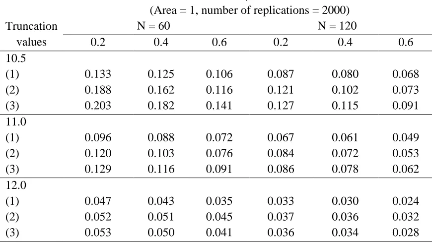
Results ...46
Discussion ...59
Limitations ...62
References ...64
iv
LIST OF TABLES
Table Page
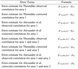
1 Computer Simulation Results: Comparisons of Mean Observed and Corrected Estimated Correlations for Different ρ Values and Truncation
Points...11
2 Computer Simulation Results: Comparisons of Mean Observed and
Corrected Estimated Correlations for ρ Values and Truncation Points ...33
3 The Number of Elements in Area 1 after Truncation ...39
4 The Areas Defining the Truncation and Robustness Situations for Area 1
and Area 2 ...39
5 Exogenous Variables Used to Define Situation in Monte Carlo Study ...41
6 Simulated Situations Used to Produce Estimated Correlations from
Thorndike’s and Alexander et al.’s Approaches. ...42
7 Error Term for Estimating Corrected Correlation Values for Thorndike’s and Alexander et al.’s Formulas ...43
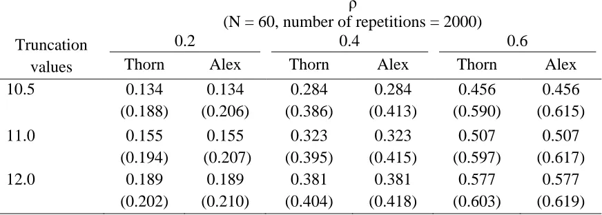
8 Comparison of the Mean Observed and Corrected Correlation Values for
Thorndike’s Approach and Alexander et al.’s Approach in Area 1 for N = 60….47
9 Mean Differences of the Observed and Corrected Correlation Values for Thorndike’s Approach and Alexander et al.’s Approach for Area 1 for
N = 60 ...47
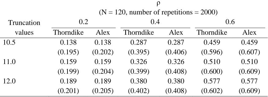
10 Comparison of the Mean Observed and Corrected Correlation Values for Thorndike and Alexander et al. in Area 1 Across 2000 Replications for
N = 120 ...48
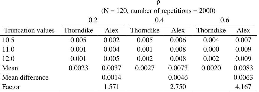
11 Mean Differences of the Observed and Corrected Correlation Values for
Thorndike and Alexander et al. for Area 1 for N = 120 ...48
12 Summary of the Absolute Values of the Mean Differences of the Observed
and Corrected Correlation Values for Area 1 for N = 60 ...49
13 Summary of the Absolute Values of the Mean Differences of the Observed
and Corrected Correlation Values for Area 1 for N = 120 ...49
14 Standard Errors of Estimated Correlations for Area 1 ...52
v
16 Mean Differences of the Observed and Corrected Correlation Values for
Area 1 and Area 2 for Thorndike and Alexander et al. for N = 60 ...54
17 Comparison of the Observed and Corrected Correlation Values in Area 1
and Area 2 ...54
18 Mean Differences of the Observed and Corrected Correlation Values for
Area 1 and Area 2 ...55
19 Summary of the Absolute Values of the Mean Differences of the Observed and Corrected Correlation Values for Area 1 and Area 2 for N = 60 ...55
20 Summary of the Absolute Values of the Mean Differences of the Observed and Corrected Correlation Values for Area 1 and Area 2 for N = 120 ...56
vi
ABBREVIATIONS
Thorndike Thorndike’s Formula
Alexander Alexander et al.’s Formula
Thorn Thorndike
T1 Thorndike Area1
T12 Thorndike Areas 1 and 2
A1 Alexander et al.’s Area 1
A12 Alexander et al.’s Areas 1 and 2
Alex Alexander et al.
CHAPTER 1
VARIOUS CORRELATION FORMULAS TO CORRECT FOR RESTRICTION OF RANGE
In this dissertation, which follows the manuscript style format approved by the
College of Education, the first chapter provides a literature review as background for the
study. Following this chapter, the second chapter employs an extended manuscript
format, supplemented by appendices, to describe the study. Many research studies
involving Pearson correlations are conducted in settings where one of the two variables
has a restricted range in a sample. For example, this occurs after tests are used for
selecting people for employment or admission to school, resulting in a distribution which
has been truncated. Often after selection, there is interest in correlating the selection
variable, which has a restricted range, to a criterion variable. The focus of this review is
on Thorndike’s (1947) correction formula and Alexander et al.’s (1984) correction
formula for use with Pearson’s correlation formula for restriction of range, although I do
mention other formulas.
Thorndike’s (1947) correction formula uses known variance for the unrestricted
situation to obtain an estimate of the corrected correlations, and Alexander et al.’s (1984)
formula with unknown variance for the unrestricted sample uses Cohen’s (1959) formula
to obtain an estimate of the unrestricted variance. In other words, Cohen’s approach,
which is incorporated in Alexander et al.’s formula, uses the restricted variance and
assumption of a normal distribution to estimate the unrestricted variance. The known
variance for the unrestricted situation in Thorndike’s formula is sometimes obtained from
In this review, there are two types of restriction of range to be considered, direct
restriction of range and indirect restriction of range. Direct restriction of range occurs
when there is a restriction of range on one of the two variables of interest. For example, if
a researcher is interested in two variables, x and y, then the restriction of range occurs on
variable x or variable y. Indirect restriction of range occurs when restriction of range
occurs on a variable other than the two variables of interest. For instance, if a researcher
is interested in two variables, x and y, then the restriction of range occurs on variable z.
Restrictions of range and cumulative meta-analysis have a strong connection because one
type of meta-analysis summarizes correlation coefficients from different studies. When
the studies involve a correlation of a test with a criterion, this form of meta-analysis is
known as validity generalization and is a potential application for Alexander et al.’s
formula.
This literature review will present Pearson’s correlation, Thorndike’s (1947)
formula, Cohen’s (1959) ratio, Alexander et al.’s (1984) formula using Cohen’s ratio,
direct and indirect restriction of range, restriction of range in meta-analysis, restriction of
range with attenuation, and contaminated normal as a background for the study reported
in manuscript style in Chapter 2.
Pearson’s Correlation
Pearson’s correlation is a number between 1 and +1 that measures the
relationship between the two variables. A positive number implies a positive association,
whereas a negative number implies the inverse association. Pearson’s correlation is a
measure of the relationship between two variables x and y, and it could be defined in
ρx,y = COV (x,y) / σxσy 1
with the corresponding sample correlation rx,y, given by
rx,y =
∑ ( ̅)( ̅)
( ) 2
Here, COV(x,y) is the population correlation between x and y, σx is the population
standard deviation of x, and σy is the population standard deviation of y. In the above
formula, are the sample standard deviations of x and y, respectively. The term
∑ ( ̅)( ̅)
( ) Additionally, Pearson’s correlation could be
expressed in terms of z-scores of x and y when the population means and population
standard deviations of x and y are available. Goodwin and Leech (2006) stated that the
Pearson’s correlation could be defined in terms of z-score of x and y as follows:
ρx,y = ∑ (zxzy) / N 3
where zx is the z-score of the x variable, calculate using the population μx, and
standard deviation σx,
zy is likewise the z-score of the y variable, and
N is the number of pairs of scores.
The square of the correlation or the coefficient of determination (i.e., ) explains the
portion of the shared variance, or the fraction of variance in one variable, x, that could be
explained by the other variable, y. Furthermore, Rodgers and Nicewander (1988)
suggested 13 different ways of interpreting a correlation value. Some of most common
ways included the interpretation of a correlation value (1) as the standardized slope of the
regression line in a z-score format, (2) as the proportion of variability in common
added a 14th way to interpret the correlation value as the proportion of matches of the
two variables of interest, x and y.
Thorndike’s Formulas for Restriction of Range
Thorndike (1947) presented formulas for correcting restriction of range for
Pearson’s (1904) formula. Thorndike developed three formulas to calculate the restriction
of range under different circumstances.
Thorndike’s Formula 1
The first formula is used to estimate the correlation between two variables of
interest, x and y, when the range of restriction occurs on variable y; the observed
correlation between the two variables of interest, x and y, is known; and the standard
deviations of the unrestricted sample and the restricted sample of variable y are also
known. Thorndike’s Formula 1 is expressed as
= √
( ) 4
where = correlation between variables x and y in an unrestricted
sample,
= correlation between variables x and y in a restricted sample, = standard deviation of the variable y in an unrestricted sample,
and
= standard deviation of the variable y in a restricted sample.
It should be noted that the ratio of restricted standard deviation to unrestricted standard
deviation is not on the variable for which the restriction occurred. Thorndike (1947)
Thorndike’s Formula 2
Thorndike’s second formula estimates the correlation between the two variables
of interest, x and y, when the restriction of range occurs at variable x; the observed
correlation value between the variables of interest, x and y, is available; and the standard
deviations of the unrestricted and restricted distribution x are also known. Thorndike’s
Formula 2 is
=
( )
√ (
)
5
where rx,y unrestricted is the correlation of x and y in an unrestricted sample,
is the correlation of x and y in a restricted sample,
SDx unrestricted is the standard deviation of variable x in an unrestricted sample, and
SDx restricted is the standard deviation of variable x in a restricted sample.
In contrast to Formula 1, Thorndike’s Formula 2 is for situations where the
required information about restricted standard deviation to unrestricted standard deviation
is on the same variable that had restricted range. Formula 2 is commonly used in
real-world situations. For example, Oleksandr and Deniz (1999) illustrated a case when
Thorndike’s (1947) Formula 2 was used in the Graduate Record Examination (GRE)
validation studies with students who were already enrolled at the school. Because the
selection was based on GRE scores, the range of scores of the students is restricted (i.e.,
most of the GRE scores in the sample are high). In general, no criterion information is
available for low-scoring persons because these applicants are not admitted to the
score and the graduate performance criterion in the restricted sample of the students that
are already enrolled at the school, they cannot compute the correlation for the total group
of applicants who applied to the graduate school. Thus, the correlation for the total group
of graduate applicants is not immediately available using Pearson’s correlation formula
alone. Thorndike’s (1947) Formula 2 was used to estimate the corrected correlation from
an unrestricted sample (i.e., the total group of applicants who apply to the graduate
school) from the correlation of the restricted sample (i.e., the correlation of students who
are already admitted to the graduate program).
Thorndike’s Formula 3
Alexander et al. (1990) note that there are two types of restrictions of range: (1)
the direct restriction of range and (2) the indirect restriction of range. The direct
restriction of range occurs when there is a restriction of range at one of the two variables
of interest; for example, if there are two variables of interest, x and y, the range
restriction occurs on variable x. The indirect restriction of range occurs at some third
variable, z, other than the two variables of interest, x and y. Thorndike’s indirect
restriction of range Formula 3 is
=
( ⁄ )
√ (( ⁄ ) ) (( ⁄ ) ) 6
where = correlation of x and y in an unrestricted sample,
= correlation of x and y in a restricted sample,
= standard deviation of the variable i in an unrestricted sample,
and
In some situations, the observed correlation value between variables x and z is not
known, and Formula 3 is expressed in terms of the correlation between variables x and z.
Thus, Thorndike’s (1947) indirect restriction of range formula could be rewritten as
=
√ ( ) ( )
√ ( )
7
where = correlation between variables i and j in an unrestricted sample,
= correlation between variable i and j in a restricted sample,
= standard deviation of the variable i in an unrestricted sample, and = standard deviation of the variable i in a restricted sample.
Thorndike’s (1947) third formula (Formula 3), an indirect restriction of range
formula, addresses correcting the correlation between the two variables of interest, x and
y, when the restriction of range occurs at a third variable, z. Additionally, Thorndike’s
Formula 3, the indirect restriction of range, estimates the corrected population correlation
between the variables of interest, x and y, when the following are known: (1) the
observed correlation values between the variables x and z and between y and z, (2) the
standard deviation of z in the unrestricted sample, and (3) the standard deviation of z in
the restricted sample.
The Cohen Ratio
Cohen (1959) proposed a ratio of sample variance in the restricted sample over
the square of difference between the sample mean in the restricted sample and the point
Cohen ratio = (
) 8
where is the sample variance in a restricted sample,
is the mean in a restricted sample, and
is the highest sorted x value in a restricted sample.
To apply this formula, sort in ascending order the array of elements of the restricted
sample from the lowest value to the highest value. The value is the highest
sorted value in the restricted sample.
The Cohen ratio is used to find the restricted standard normal standard deviation
and the z-score from Cohen’s table (see Appendix B). Cohen’s table is based on the fact
that his formula results in a unique value for truncation point . More
specifically, the Cohen table has three columns. The first column is the Cohen ratio; the
second column represents the table restricted normal standard deviation (i.e., SDtab),
which is the “standardized value of the standard deviation after truncation (with a non-
truncated value of 1.0). That table value also represents the proportion reduction in
standard deviation due to range restriction” (Alexander et al., 1984, p. 432). The third
column in the Cohen table represents the z-score. From the table, the restricted normal
standard deviation value and its z-score are found by doing a table look-up based on
Cohen’s ratio.
Alexander et al.’s Formula
Since the unrestricted standard deviation is not directly known in Alexander,
Alexander et al.’s (1984) formula uses the Cohen ratio to obtain the SDtab value from
Cohen’s table (see Appendix B). As Alexander et al. (1984) points out, “Cohen’s ratio
is obtained, Alexander et al.’s formula estimates the unrestricted standard deviation based
on the values of the observed standard deviation in the restricted sample and the table
restricted normal standard deviation in the restricted sample. Alexander et al.’s formula
estimates the unrestricted standard deviation as follows:
= / 9
where is the estimate of the unrestricted standard deviation,
is the observed standard deviation in the restricted sample, and
stands for avalue for the restricted normal standard deviation.
The and values will then be used to calculate the U ratio, which in turn will be
used to estimate the corrected correlation using Thorndike’s (1947) Formula 2. Using the
U ratio and Thorndike’s (1947) Formula 2, Alexander et al. (1984) developed the
following formula:
= (r *
) / SQRT (1 - ( (
) )) 10
where is the corrected correlation value,
r is the observed correlation value in the restricted sample, is the estimate of the unrestricted standard deviation, and is the observed standard deviation in the restricted sample.
Alexander et al. (1984) employed a Monte Carlo computer simulation program to
compare the means of the observed correlation values with the corresponding means of
the corrected estimated correlations using his formula. In his computer simulation
0.4, 0.6, 0.8), and various truncation values (i.e., 2.0, 1.5, 1.0, 0.5, 0, 0.5, 1.0). The
computer simulation produced the table of comparison between the two means (i.e.,
observed correlation values and the corrected correlation values), which is presented in
Table 1. Alexander et al. did not investigate non-normality nor did he compare his mean
correlation estimates with estimates from Thorndike’s formula.
Even though the unrestricted variance was estimated through Alexander et al.’s
(1984) formula, in every case except for the truncation value at −2.0, the results of the
mean estimated corrected correlation values were closer to the true ρ correlation values
than the mean observed correlation values, as can be seen in Table 1. Similarly, in every
case except for the severe cut (i.e., +1.0), the mean estimated corrected correlation value
was an over estimate for truncation values (i.e., 2.0, 1.5, 1.0, 0.5, 0, +0.5). The
overestimations were either 0.01 or 0.02. For the severe cut, the mean estimated corrected
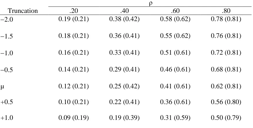
Table 1
Computer Simulation Results from Alexander et al.: Comparison of Mean Observed and Corrected Estimated Correlations for Different ρ Values and Truncation Points
ρ
Truncation .20 .40 .60 .80
2.0 0.19 (0.21) 0.38 (0.42) 0.58 (0.62) 0.78 (0.81)
1.5 0.18 (0.21) 0.36 (0.41) 0.55 (0.62) 0.76 (0.81)
1.0 0.16 (0.21) 0.33 (0.41) 0.51 (0.61) 0.72 (0.81)
0.5 0.14 (0.21) 0.29 (0.41) 0.46 (0.61) 0.68 (0.81)
µ 0.12 (0.21) 0.25 (0.42) 0.41 (0.61) 0.62 (0.81)
+0.5 0.10 (0.21) 0.22 (0.41) 0.36 (0.61) 0.56 (0.80)
+1.0 0.09 (0.19) 0.19 (0.39) 0.31 (0.59) 0.50 (0.79)
Note. Corrected correlation values using Alexander et al.’s formula are in parentheses. Data presented are mean correlations for samples with N = 60 for 5,000 replications. This table was taken from Alexander et al. (1984). Permission is found in Appendix D.
Alexander et al. (1984) also used the estimate unrestricted standard deviation,
z-score, and the highest sorted value of x from the previous equation to derive a formula to
correct mean. Alexander et al.’s corrected mean formula is as follows:
̅= - z 11
where ̅ is the corrected mean,
is the highest sorted x value in in a restricted sample,
z is the z-score from the Cohen’s table, and
is the estimated unrestricted standard deviation.
Thus, Alexander et al.’s (1984) formula is a special case of Thorndike’s (1947)
presented as population values, but in Alexander et al.’s version, the restricted variance is
estimated from the sample and the unrestricted variance needs to be estimated from the
sample variance. Consequently, Alexander et al. employed Cohen’s (1959) ratio formula
to obtain the estimate of the unrestricted variance. From the estimated unrestricted
variance, Alexander et al. computed the U ratio, which was then entered into the
Thorndike’s (1947) Formula 2 to estimate the corrected correlation value.
Attenuation in Restriction of Range
Sackett and Yang (2000) stated that there are two common methods for correcting
correlation values in a direct restriction of range and an indirect restriction of range.
Hunter and Schmidt (2004) mentioned that majority of correlation values are not true
correlation values because they are in fact lowered by error of measurement. Stauffer and
Mendoza (2001) suggested a formula for correcting correlation for range restriction and
unreliability. Additionally, Hunter, Schmidt, and Le (2006) proposed the Hunter-Schmidt
corrected correlation with attenuation for the direct and indirect restriction of range.
Further, Raju et al. (2006) suggested another method for corrected correlation with
attenuation based on the reliabilities of x and y in a restricted sample. Before discussing
these formulas, a brief overview of basic classical test theory is presented.
Reliability
A true score can be stated in terms of the observed score and its measurement
error. For example, if a researcher observed a score on a test denoted by x, and there is an
error of measurement associated with it called ex (i.e., ex is measurement error of variable
x), then the observed score of x could be written as
where tx is the true score for variable x.
In classical test theory, the amount of error of measurement in the variable is
measured by the number called the reliability of the variable, denoted for variable x as
rxx. The reliability of an observed test score consists of two components: the true score
and some form of error measurement (Donald, Lucy, & Asghar, 1990). Given some
assumptions, it has been shown that the variance of the observed scores (σx2) is equal to
the variance of the true scores (σt2) plus the variance of their errors of measurement (σe2)
(Donald et al.). This can be expressed as
σx2 = σt2 + σe2 13
Reliability can be defined as a ratio of true score variance over the observed score
variance. That is, reliability, rxx, is equal to
rxx = σt2 / σx2 14
Reliability ranges from 0 to 1, where a reliability of 1 indicates no error. Using equation
13, formula 14 can be rewritten as
rxx = 1 - σe2/σx2 15
Hunter and Schmidt (1990) stated that reliability measures the percentage of the observed
variance, which is the true score variance. For example, if the reliability of variable x is
0.8, it is implied that 80% of the variance in variable x is due to the true score variation
and the remainder 20% of the variance in variable x belongs to measurement error.
Attenuation Formulas
Correction for attenuation is a statistical procedure, according to Spearman
(Jensen, 1998). Given the fact that the correlation between variables of interest, say x and
y, is diluted by measurement error, the correction for attenuation procedure, it has been
argued, provides a more accurate estimate of the correlation between variables x and y by
accounting for this effect.
Before presenting corrections for attenuation, the general form of the correction
approach advocated by Hunter and Schmidt (2004) for a form of meta-analysis called
“validity generalization” is presented. As stated earlier, since measurement error in
correlation is associated with artifacts, those artifacts can be addressed in terms of
correcting correlation with attenuation (Schmidt & Huy, 2006). The following corrected
correlation could be expressed as
ρ’ = aρ 16
where ρ’ is the corrected population correlation with attenuation,
a is the artifact, and
ρ is the population correlation before attenuation.
Furthermore, if there is a second artifact associated with the population correlation before
attenuation, the above formula could be rewritten to incorporate the additional artifact as
follows:
ρ’ = a1 a2ρ 17
where ρ’ is the corrected population correlation with attenuation,
a1 is the artifact,
a2 is the artifact, and
Thus, if there are n artifacts associated with the correct correlation with attenuation, then
the formula would become
ρ’ = a1 a2…anρ 18
where ρ’ is the corrected population correlation with attenuation,
a1 is the artifact,
a2 is the artifact,
an is the artifact, and
ρ is the population correlation before attenuation.
Based on the correlation with attenuation, Schmidt, Le, and Illies (2006) proposed a
formula to include measurement error in the estimate of the parameter in an unrestricted
population from the parameter in a restricted population.
Hunter-Schmidt’s Correlation with Attenuation Formulas
Hunter et al. (2006) discussed the error of estimate of an unrestricted population
correlation through Thorndike’s case two and case three. Thorndike’s (1947) case two
formula is widely used in the correction for the direct range of restriction of two variables
of interest, x and y, where the restricted sample correlation is known between the two
variables, and the correction factor or the sample standard deviation of the unrestricted
and the restricted populations are known for one of the parameters. Similarly, there is
also a range restriction with attenuation formula for Thorndike’s (1947) case three
formula, which is used for the indirect range of restriction. In Thorndike’s case three
formula, the restriction occurs on the third variable, z, which is correlated to both
Hunter et al. (2006) developed a range restriction with attenuation formula to
address the measurement error of the direct range of restriction for Thorndike’s (1947)
case two formula:
ρ’ = ρ 19
where is the attenuation coefficient for the correct correlation with attenuation, and it
could be expressed as
= ( ) 20
is the U ratio and it was defined as the ratio of ⁄ ,
and ρ is defined as the product of ρtx,ty, and (SQRT (rxxryy)) where rxx and ryy are the
reliabilities of variables x and y (Hunter & Schmidt, 1999). Furthermore, Hunter et al.
(2006) also discussed the range restriction with attenuation for the indirect range
restriction.
Hunter and Schmidt’s Formula on Range Restriction with Attenuation for Indirect
Range Restriction
Hunter et al. (2006) proposed a formula to range restriction with attenuation for
the indirect range restriction by giving detailed instructions on how to incorporate
measurement error and reliability into the existing Thorndike’s formula. The steps are as
follows:
Step 1: Estimating the reliability of the independent variable x in the restricted
population.
= 1 - (1 - ) 21
where is the U ratio , and
Step 2: Estimating the range restriction on used of correcting factor , and the
reliability of independent variable x
= √ ( ) ⁄ 22
where is the U ratio , and
is the reliability of the unrestricted x variable,
Step 3: Correcting for measurement error before applying restriction of range correction
= r / √ 23
where r is the correlation before attenuation.
Step 4: Applying Thorndike case 2 formulas using equations from Step 3 and Step 2
=
√ 24
Besides Hunter and Schmidt’s (2006) formulas for correct correlation formulas,
Stauffer and Mendoza (2001) suggested a new method for the range restriction with
attenuation.
Stauffer and Mendoza’s Formula
Stauffer and Mendoza (2001) proposed a formula for correcting correlation for
range restriction and unreliability, which was based on Thorndike’s Formula 2 with the
available estimates: (1) the unrestricted predictor reliability, (2) the incident range
restricted criterion reliability, and (3) the restricted correlation. Stauffer and Mendoza’s
(2001) correcting correlation for range restriction and unreliability is defined as follows:
=
√ √
25
where is the U ratio,
is the unrestricted predictor reliability, and
is the incident range restricted criterion reliability.
Thus, since correction formula and unreliability are common in real-world
situations, Stauffer and Mendoza (2001) developed a rule of thumb for determining an
order to handle the corrections by looking at the nature of the reliability estimate. Further,
Raju et al. (2006) developed new approach for corrected correlation based on reliabilities.
Raju, Lezotte, Fearing, and Oshima’s Formula
Raju et al. (2006) proposed a method to calculate the corrected correlation based
on the reliability of x and y in a restricted sample:
= k / √ 26
where is the reliability of independent variable x,
is the reliability of the dependent variable y,
is the correlation value of x and y in a restricted sample, and
k is defined as the ratio of unrestricted true scores standard deviation over the
restricted true scores standard deviation.
In other words, k is defined as follows:
k = / 27
Raju et al. (2006) offer a procedure for estimating corrected correlation in range
restriction for unreliability when an estimate of the reliability of a predictor is not
available for the unrestricted sample. It has been long recognized that measurement error
since Thorndike’s day, researchers have been correcting correlation based on
measurement errors and restriction in range (Mendoza & Mumford, 1987). This topic has
received considerable attention in recent years, with a new correction formula for
attenuation from Hunter et al. (1990) and even more recently from Raju et al. (2006).
These new correction formulas help ease the measurement error for corrected correlation
in the restriction of range. Meta-analysis uses different type of corrections; thus, when
applying the restriction of range to meta-analysis, the meta-analysis summary would
result in a better understanding of what the correlations are in the unrestricted situations.
Meta-Analysis
Meta-analysis, a procedure for summarizing empirical studies, can be employed
to summarize Pearson’s correlation; it can be generally defined by the following steps:
(a) defining a topic area and criteria for admissible studies, (b) locating relevant primary
research, (c) coding study characteristic, (d) measuring study results on a common scale,
and (e) aggregating the study results and relating them to study characteristics (Matheny,
Aycock, Pugh, Curlette ,& Cannella, 1985). Additionally, meta-analysis can also be used
as a guide to answer the question about what a researcher should be doing to incorporate
one study with another study even if the first study employs different instruments across a
different range of people (Hunter & Schmidt, 1990). Furthermore, Hunter and Schmidt
(2004) stated that every method of meta-analysis is based on the theory of data, and a
complete theory of data includes an understanding of sampling error, measurement error,
and bias sampling in case of range restriction. The estimation of sampling error in
meta-analysis could be expressed as the weight average in each correlation, which is weighted
̅ = ∑
∑ 28
where is the correlation in study i, and
is the number of persons in study i.
Hunter and Schmidt (2004) stated that the corresponding variance across studies is not
the usual sample variance, but the frequency-weighted average squared error. The
formula could be derived in term of the above equation as follows:
∑ ∑ ( ̅) 29
where is the correlation in study i,
̅ is the weighted average,
is number of persons in study i, and
N is total number of persons.
Furthermore, other correction formulas that focus on the measurement error and bias
sampling could be addressed by the earlier work of Hunter and Schmidt correction
formula with attenuation on range restriction for direct and indirect restriction of range in
the previous section.
Contaminated Normal
Contrary to the general belief that correlation value in a restricted sample tends to
be smaller than the correlation value in the unrestricted sample, Zimmerman and
Williams (2000) state that the correlation in the restricted sample is sometimes larger
than the correlation in the unrestricted sample. This happens in a class called the
“contaminated normal,” in which the assumption of normal distribution is violated in a
particular way. In a contaminated normal situation, scores of outliers increase the
Standard Error
Cochran (1977) suggested a mean square error (MSE) formula to compare a
biased estimator with an unbiased estimator or the two biased estimators that could be
presented as the expected value of the square of the difference between the estimated
population correlation value and the true population correlation value:
MSE = E (ρ̂ – ρ)2 30
where ̂ is the estimated population correlation value and ρ is the population correlation
value. Additionally, when the estimated population correlation value approaches the
mean population correlation value, the MSE could be expressed in terms of the mean of
the population correlation values, such as
MSE = E [( ̂ ) + (m - ρ)]2
31
MSE = E ( ̂ )2 + 2 (m - ρ) E( ̂ ) + (m - ρ)2
32
Since the expected value of the difference of the estimated population correlation value
and the mean of population correlation equals to zero, the MSE could be simplified to
MSE = E ( ̂ )2
+ (m - ρ)2 33
Thus, the MSE could be expressed in terms of variance of ̂ and bias, where
E ( ̂ )2 is the variance of ̂ ,
(m - ρ)2 is the bias,
̂ is the estimated population correlation value,
ρ is the true population correlation value, and
Furthermore, the standard error can be derived from the MSE as the square root (SQRT)
of the MSE, where the standard error equals to the SQRT (MSE).
Summary
Restriction of range is a frequent topic in education and other areas where there is
a selection process and criterion-related validity using Pearson’s correlation is desired.
Thorndike’s (1947) and Alexander et al.’s (1984) formulas use the original Pearson’s
correlation formula to develop their corrected correlation formulas for restriction of
range. As stated earlier, Thorndike’s formula uses known variance for the unrestricted
situation to obtain an estimate of the corrected correlation, whereas Alexander et al.’s
formula with unknown unrestricted variance uses the Cohen ratio formula to obtain the
population variance, and then it uses the population variance in Thorndike’s Formula 2 in
order to obtain the estimated corrected correlation. Hunter and Schmidt (2004) stated that
the majority of correlation values were not true correlation values because they were in
fact lowered by error of measurement. Thus, because of unreliability, since Thorndike’s
day, researchers have been correcting correlation based on measurement errors and
restriction in range (Mendoza, Hart, & Powell, 1994). Furthermore, correcting correlation
based on measurement errors has received considerable attention in recent years with new
correction formulas for attenuation from Hunter and Schmidt (1990), Mendoza et al.
(1994), and most recently from Raju et al. (2006). Those new correction formulas help
ease the measurement error for corrected correlation in the restriction of range. For
example, works on corrected correlation in restriction of range with attenuation have
been shown through Hunter and Schmidt’s formulas for direct and indirect restriction of
corrected correlation with attenuation. Also, meta-analysis uses different types of
corrections; thus, applying the restriction of range to meta-analysis would result in a
better understanding of what correlations are in unrestricted situations. This literature
review included restriction of range formulas, restriction of range with attenuation
formulas, meta-analysis, and contaminated normal as a background of the following
References
Alexander, R. A., Alliger, G. M., & Hanges, P. J. (1990). Correcting for range restriction
when the population variance is unknown. Applied Psychological Measurement,
8, 431437.
Alexander, R. A., Hanges, P. J., & Alliger, G. M. (1984). Correcting for restriction of
range in both x and y when the unrestricted variances are unknown. Applied
Psychological Measurement, 8(4), 431437.
Cochran, G. W. (1977). Sampling techniques. New York: John Wiley & Sons.
Donald, A., Lucy, C. J., & Asghar, R., (1990). Introduction to research in education.
Forth Worth, Texas: Harcourt Brace College Publisher.
Goodwin, D. L., & Leech. L. N. (2006). Understanding correlation: Factors that affect the
size of r. The Journal of Experimental Education, 74(3), 251266.
Hunter, J. E., Schmidt, F. L., Le, H. (2006). Implication of direct and indirect
range restriction for meta-analysis methods and findings. Journal of Applied
Psychology, 91(3), 594612.
Hunter, J. E., & Schmidt. L. F. (2004). Methods of meta-analysis: Correcting error and
bias in research findings. Thousand Oaks, CA: Sage Publications.
Hunter, J. E., & Schmidt, L. F. (1990). Methods of meta-analysis: Correcting error and
bias in research findings. Thousand Oaks, CA: Sage Publications.
Jensen, A.R. (1998). The g factor: The science of mental ability. Mahwah, NJ:
Lawrence Erlbaum & Associates.
Lipsey, M. W., & Wilson, D. B. (2000). Practical meta-analysis. Applied social research
Matheny, K. B., Aycock, D. W., Pugh, J. L., Curlette, W. L., & Cannella, K. A. S.
(1986). Stress coping: Qualitative and quantitative synthesis with implications for
treatment. The Counseling Psychologist, 14(4), 499549.
Mendoza, J. L, Hart, D. E., & Powell, A. (1994). Explanations for accuracy of the general
multivariate formulas in correcting for range restriction. Applied Psychological
Measurement, 18, 355367.
Mendoza, J. L., & Mumford, M. (1987). Corrections for attenuation and range restriction
on the predictor. Journal of Educational Statistics, 12(3), 282293.
Oleksandr, S. C., & Deniz S. O. (1999). How selective are psychology graduate
programs? The effect of the selection ratio on GRE scores validity. Educational
and Psychological Measurement, 59, 951961.
Pearson, K. (1903). Mathematical contribution to the theory of evolution-XI. On the
influence of natural selection on the variability and correlation of organ. Phil.
Trans. Royal Soc. of London, Series A, 200, pp 166.
Raju, N. S., Lezotte, D. V., Fearing, B. K., & Oshima, T. C. (2006). A note
on correlations corrected for unreliability and range restriction. Applied
Psychology Measurement, 30(2), 145149.
Rodgers, J. L., & Nicewander, W. L. (1988). Thirteen ways to look at the correlation
coefficient. The American Statistician, 42, 59–66.
Rovine, M. J., & Von, E. A. (1997). A 14th way to look at a correlation coefficient:
Correlation as the proportion of matches. The American Statistician, 51, 4246.
Sackett, P. R., & Yang, H. (2000). Correction for range restriction: An expanded
Schmidt, F. L., & Huy, L. (2006). Increasing the accuracy of corrections for range
restriction: Implication for selection procedure validities and other research
results. Personal Psychology, 59, 281305.
Schmidt, F. L., Le, H., & Illies, R. (2003). Beyond alpha: An empirical examination of
the effects of different sources of measurement error on reliability estimates for
measures of individual differences constructs. Psychological Methods, 8,
206224.
Stauffer, M. J., & Mendoza, L. J. (2001). The proper sequence for correcting correlation
coefficients for range restriction and unreliability. Psychometrika, 66, 6368.
Thorndike, R. L. (1947). Research problems and techniques (Rep. No. 3 AAF Aviation
Psychology Program Research Reports). Washington, DC: U.S. Government
Printing Office.
Zimmerman, D. W., & Williams, R. H. (2000). Restriction of range and correlation in
CHAPTER 2
A COMPARISON OF ROBUSTNESS OF THORNDIKE’S AND AN ADAPTATION OF COHEN’S FORMULA TO CORRECT FOR RESTRICTION OF RANGE
The focus of this research was to compare Alexander et al.’s formula to
Thorndike’s formula and to population values using Monte Carlo simulation when the
assumption of a normal distribution is violated in a particular way. Many research studies
involving Pearson’s correlations are conducted in settings where one of the two variables
has a restricted range in a sample. For example, this occurs when tests are used for
selecting people for employment or admission to school. Often after selection, there is
interest in correlating the selection variable, which has a restricted range, to a criterion
variable in order to obtain criterion-related validity using Pearson’s correlation. Since the
restriction of range situation occurs in many settings and Pearson’s correlation is
fundamental to many statistical procedures, the accuracy of correction approaches for
restriction of range can relate to many statistical procedures. A particular statistical
procedure for which these correction procedures have potential application is validity
generalization, which is a form of meta-analysis.
A unique feature of the current study is the way in which the robustness situations
are defined. They are defined from the perspective of a statistical classification problem
for two groups and one variable on which to make the classification decision. Group 1
has a normal distribution on variable X and is referred to as distribution 1. Likewise,
group 2 has been measured on variable X and has a normal distribution, designated as
distribution 2. Both distributions have the same population standard deviations but
In this classification problem, after the classification decision is made, there are
two potential errors of classification: (1) an individual from group 1 is misclassified into
group 2 and (2) an individual from group 2 is misclassified into group 1. There could be a
desire to identify individuals who are predicted to be in group 1 when the classification
rule is applied to a new group of people. Suppose, for example, that the task was to
predict people leaving a job based on the supervisor’s rating after two years of
employment. The supervisor’s ratings of employees would be obtained after one year of
employment, and the employees’ work statuses in the organization would be obtained at
the end of the second year. Then, a classification rule would be obtained to predict which
employees would stay and which employees would leave. Given two normal distributions
and one predictor variable, the cut point for the classification rule on rating variable, X,
would be halfway between the mean of the two distributions without consideration of
prior probabilities. Now, a new group of employees comes along, and it is desired to
study the correlations between those predicted to stay with another variable of interest,
for example, Y. Those predicted to stay make a mixed distribution of group 1 and group
2. In particular, those individuals from distribution 1 below the cut point constitute group
1, along with those individuals from group 2 who have been misclassified because they
are below the cut point. An illustration of the classifying problem is shown by Figure 1,
Figure 2, and Figure 3 presented in Appendix F. In this fashion, the robustness situations
for the restriction of range situations are defined for the Monte Carlo simulation.
Two other contributions of this research are to (1) compare the accuracy of
Thorndike’s (1947) case 2 formula to Alexander et al.’s (1984) formula based on point
In his article, Alexander et al. (1984) compares estimates of correlations based on
Cohen’s approach to population correlation values and not to estimates from Thorndike’s
formula. After a brief review of the literature in the background section, I identify the
exogenous variables to define the simulated situations and provide a more detailed
description of the robustness situations that will be described in the methodology section.
Background
Thorndike’s Direct Restriction of Range Formula
Thorndike (1947) introduced the corrections for restriction of range. Thorndike’s
Formula 2 estimates the population correlation between two variables of interest, X and
Y, when the restriction of range has occurred on variable X. Thorndike’s Formula 2 is
shown as follows:
=(( ) (
)) ( (
)) 30
where is the corrected correlation for the unrestricted restriction of range,
is the restricted range correlation,
SDu is the unrestricted standard deviation, and
SDrest is the restricted standard deviation.
The ratio of SDu over SDrest is defined as the U ratio or the correcting factor. The
U ratio for Thorndike’s formula is defined as the ratio of the unrestricted standard
deviation over the restricted standard deviation. Thorndike’s Formula 2 is designed for
situations where the required information about restricted standard deviation to
unrestricted standard deviation is on the same variable that had restricted range. In
variance for the unrestricted situation to obtain an estimate of the corrected correlations.
Oleksandr and Deniz (1999) provides a case when Thorndike’s (1947) Formula 2 was
used in Graduate Record Examination (GRE) validation studies in which the researcher
was interested in estimating the corrected correlation from an unrestricted sample from
the correlation of the restricted sample. Additionally, Thorndike’s (1947) case two
formula is widely employed in personnel selection for employment, when the test scores
used for new applicants are related to job performances (Viswesvaran, Ones, & Schmidt,
1996; Schmidt & Hunter, 1998). In this study, selection was made on the scores; thus, the
range of scores was restricted in the sample. Even though the correlation between test
score and job performance could have been obtained from the restricted sample, the
researcher still wanted to know the correlation in the unrestricted sample (Henriksson &
Wolming, 1998; Hunter & Schmidt, 1990). Hence, Thorndike’s (1947) Formula 2 has
been used in many instances in real-world situations ranging from educational research to
employment, and it has been shown to produce close estimates of the correlation in the
population (Oleksandr & Deniz, 1999).
The Cohen Ratio
Cohen (1959) based his formula on the sample variance in the restricted sample
over the square of difference between the sample mean in the restricted sample and the
point of truncation in the restricted sample. The formula for the Cohen ratio can be
presented as
Cohen ratio = ( ) 31
is the mean of the restricted sample , and
is the point of truncation in the restricted sample.
Alexander et al. (1984) points out that Cohen’s ratio has an advantage over others’
formulas because it needs only the variance of the restricted sample, the mean of the
restricted sample, and the highest observed Xc in the restricted sample. The value Xc can
be obtained from an ascending-ordered array where all X scores could be stored in an
unordered array, and the unordered array could be sorted by an efficient sorting algorithm
named quick sort (Horowitz & Sahni, 2000). Thus, once the Cohen ratio is determined,
the z-score and table restricted normal standard deviation, named SDtab, could be
obtained from the Cohen table, which has three columns (see Appendix B). The first
column is the Cohen ratio, the next column is the SDtab, and the last column is the
z-score. The SDtab, and z-score would be found from the Cohen table by performing a table
look-up of the Cohen ratio.
Cohen’s Ratio in Alexander et al.’s Formula
Thorndike’s (1947) case two formula assumes that the variance of variables in the
unrestricted area is known, whereas in Alexander et al.’s formula, the unrestricted
variance is unknown. With the unknown variance in the unrestricted sample, Alexander
suggested a method for estimating the unrestricted standard deviation using the Cohen
ratio. Alexander et al. (1984) used the Cohen ratio in the previous equation to obtain the
z-score and the SDtab (as seen in the Cohen table in Appendix B). Once the value
was obtained, Alexander et al.’s (1984) formula was then employed to estimate the
unrestricted standard deviation as follows:
where is the unrestricted standard deviation,
is the observed standard deviation in the restricted sample, and
SDtab is the tabled restricted normal standard deviation in restricted sample.
Once the estimates of the unrestricted standard deviation, the observed standard
deviation, and the restricted correlation are available, the estimate corrected correlation
could be calculated using Thorndike’s Formula 2. An example of the Monte Carlo
computer simulation program of the comparison of the mean observed and corrected
correlations for different population’s correlation and truncation values is given in Table
2. Even though the unrestricted variance was estimated through Alexander et al.’s (1984)
formula, in every case except for the truncation value at −2.0, the results of the estimated
corrected correlation values were closer to the true ρ correlation values than the observed
correlation values. Likewise, in every case except for the severe cut (i.e., +1.0), the
estimated corrected correlation value was an overestimate for truncation values (i.e.,
2.0, 1.5, 1.0, 0.5, 0, +0.5). The overestimations were either 0.01 or 0.02. Thus, the
results show that Alexander et al.’s formula is a worthwhile estimate of corrected
correlation in a real-world situation where more than often, the variance of the
unrestricted sample is not given and the researcher could estimate it using the Cohen
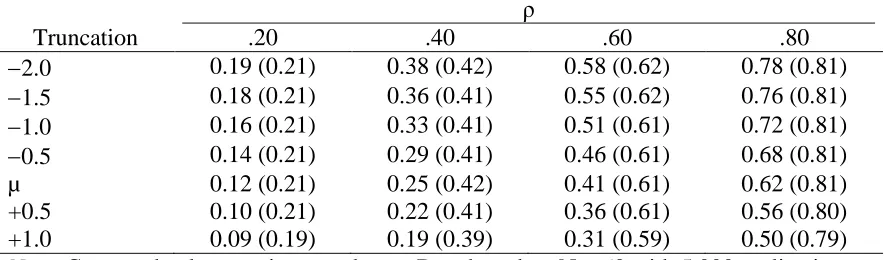
Table 2
Computer Simulation Results: Comparison of Mean Observed and Corrected Correlations for ρ and Truncation Points
ρ
Truncation .20 .40 .60 .80
2.0 0.19 (0.21) 0.38 (0.42) 0.58 (0.62) 0.78 (0.81)
1.5 0.18 (0.21) 0.36 (0.41) 0.55 (0.62) 0.76 (0.81)
1.0 0.16 (0.21) 0.33 (0.41) 0.51 (0.61) 0.72 (0.81)
0.5 0.14 (0.21) 0.29 (0.41) 0.46 (0.61) 0.68 (0.81)
µ 0.12 (0.21) 0.25 (0.42) 0.41 (0.61) 0.62 (0.81)
+0.5 0.10 (0.21) 0.22 (0.41) 0.36 (0.61) 0.56 (0.80)
+1.0 0.09 (0.19) 0.19 (0.39) 0.31 (0.59) 0.50 (0.79)
Note. Corrected values are in parentheses. Data based on N = 60 with 5,000 replications. This table was taken from Alexander et al. (1984). Permission is found in Appendix D.
Thorndike’s and Alexander et al.’s Variances in the Unrestricted and Restricted
Situations
In both Thorndike’s and Alexander et al.’s correction formulas, values for the
variances in the restricted and the unrestricted situations are required. For both formulas,
the variance in restricted situations was a sample estimate. In the Monte Carlo simulation,
the difference between the two approaches was that in Thorndike’s formula, the variance
in the unrestricted situation was the population variance from the exogenous, whereas in
Alexander et al.’s approach, the population variance was estimated based on the sample
variance in the restricted situation. The particular method that was used to create the
robustness situations was the non-normal distributions for predicted group membership in
a classification problem. Shown in Appendix C is a table that shows the sources for the
variances in the restricted and unrestricted situations for Thorndike’s and Alexander et
Non-Normal Situations as a Result of a Classification Problem
The problem of classifying people into groups is formed on the basis of a set of
measurements, such as the aptitude tests and personal inventory scores, which often
arises in applied research psychology or social science (Johnson & Wichern, 1998;
Kuncel, Hezlett, & Ones, 2004). The particular classification problem employed to define
non-normal distribution for robustness situations is a two-group classification situation
with one predictor variable. Group 1 has a normal distribution on variable X and is
referred to as distribution 1. Likewise, group 2 has been measured on variable X also and
has a normal distribution that will be designated as distribution 2. Both distributions have
the same population standard deviations but different population means. In this
classification problem, after the classification decision is made, there are two errors of
classification; more particularly, an individual from group 1 is misclassified into group 2,
and an individual from group 2 is misclassified into group 1.Suppose it is desired to study
the individuals predicted to be in group 1, that is, those individuals below a cut point on
the predictor variable. These individuals are a mixture of group 1 and group 2, which has
a non-normal distribution.
Standard Error
Standard error is the square root of the mean square error, which can be defined as
the expected value of the square of the difference between the estimated population value
and the true population value. Cochran (1977) presented a mean square error formula
(i.e., MSE) that can be expressed as the expected value of the square of the difference
between the estimated population correlation value and the true population correlation
MSE = E (ρ̂ – ρ)2 33
The MSE could be rewritten in terms of the mean of population correlation value m as:
MSE = E ( ̂ )2
+ (m - ρ)2 34
where E ( ̂ )2 is the variance of ̂ ,
(m - ρ)2 is the bias,
̂ is the estimated population correlation value,
ρ is the true population correlation value, and
m is the mean of population correlation.
Thus, the standard error estimate could be derived from the square root of the mean
square error such as
Standard error = √ 35
Degree of Closeness of Two Correlations
Cohen (1987) suggested using Fisher’s z transformation in the computing of the
degree of closeness of the two correlations by taking the absolute value of the difference
of the two z-values that were derived from one-half of the natural log of the quotient of
(1 + r) and (1 - r); the result was then compared with Cohen’s effect size to find out the
magnitude of the closeness of the correlations:
d = | | 36
z = 0.5 ln( ) 37
where z is the Fisher’s z transformation,
Ultimately, the practical significance of the differences of two correlation corrections
compared to population values depends on how the differences affect conclusions drawn
from applied research.
Skewness
Skew can be defined as an expected value of the averaged cubed deviation from
the mean divided by the standard deviation cubed as E[( ) ], where µ is the
population mean and σ is the population standard deviation (Groeneveld & Meeden,
1984). If the skew value is greater than zero, then there is a positive skew, whereas
negative skew occurs when the result is less than zero. Additionally, it is symmetric, or
“no skew,” when the result is zero.
Research Questions
The significance of the current study is to contribute an additional understanding
of the corrections for the effect of restriction of range on correlation. Because
Thorndike’s Formula 2 uses known population unrestricted variance and Alexander et
al.’s formula has to estimate the unrestricted variance by utilizing the Cohen (1959) ratio
formula, I expected that Thorndike’s Formula 2 would provide better precision than
Alexander et al.’s formula. I investigated four research questions related to the restriction
of range:
1. How accurate in terms of point estimates of correlations are Thorndike’s
(1947) and Alexander et al.’s (1984) formulas to correct for restriction of
2. How do the standard errors of Thorndike’s corrected correlations compare to
Alexander et al.’s corrected correlations for an original normal distribution
that has been truncated?
3. In the robustness situations, how accurate in terms of point estimates of
correlations are Thorndike’s (1947) and Alexander et al.’s (1984) formulas to
correct for restriction of range?
4. In the robustness situations, how do the standard errors of Thorndike’s (1947)
corrected correlations compare to the standard errors of Alexander et al.’s
(1984) corrected correlations?
Methodology
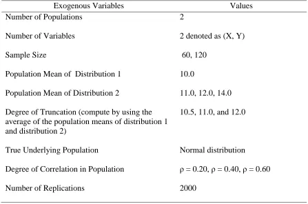
The robustness situations for restriction of range situations are defined for the
Monte Carlo simulation from the perspective of a statistical classification problem for
two groups and one variable on which to make the classification decision. Group 1 has a
normal distribution on variable X and is referred to as distribution 1. Likewise, group 2
has also been measured on variable X and has a normal distribution, designated as
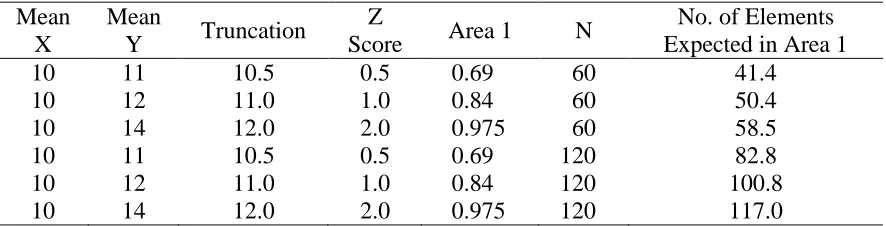
distribution 2. Both distributions have the same population standard deviations of 1.0 but
different population means. Group 1 has a population mean of 10.0, and group 2 has the
following population means: 11.0, 12.0, and 14.0. The cut points for classifying an
observation into group 1 and group 2 are the average of the population mean of group 1
and the population mean of group 2. The values of the cut points are 10.5, 11.0, and 12.0.
The corresponding z-score for the cut points are 0.5, 1.0, and 2.0, referenced from