www.hydrol-earth-syst-sci.net/19/2911/2015/ doi:10.5194/hess-19-2911-2015
© Author(s) 2015. CC Attribution 3.0 License.
Operational aspects of asynchronous filtering for flood forecasting
O. Rakovec1,3, A. H. Weerts1,2, J. Sumihar2, and R. Uijlenhoet1
1Hydrology and Quantitative Water Management Group, Department of Environmental Sciences, Wageningen University,
Wageningen, the Netherlands
2Deltares, P.O. Box 177, 2600 MH Delft, the Netherlands
3UFZ – Helmholtz Centre for Environmental Research, Leipzig, Germany
Correspondence to: O. Rakovec ([email protected])
Received: 14 February 2015 – Published in Hydrol. Earth Syst. Sci. Discuss.: 20 March 2015 Revised: 05 June 2015 – Accepted: 08 June 2015 – Published: 23 June 2015
Abstract. This study investigates the suitability of the asyn-chronous ensemble Kalman filter (AEnKF) and a partitioned updating scheme for hydrological forecasting. The AEnKF requires forward integration of the model for the analysis and enables assimilation of current and past observations simul-taneously at a single analysis step. The results of discharge assimilation into a grid-based hydrological model (using a soil moisture error model) for the Upper Ourthe catchment in the Belgian Ardennes show that including past predictions and observations in the data assimilation method improves the model forecasts. Additionally, we show that elimination of the strongly non-linear relation between the soil mois-ture storage and assimilated discharge observations from the model update becomes beneficial for improved operational forecasting, which is evaluated using several validation mea-sures.
1 Introduction
Understanding the behaviour of extreme hydrological events and the ability of hydrological modellers to improve the fore-cast skill are distinct challenges of applied hydrology. Hy-drological forecasts can be made more reliable and less un-certain by recursively improving initial conditions. A com-mon way of improving the initial conditions is to make use of data assimilation (DA), a feedback mechanism or update methodology which merges model estimates with available real-world observations (e.g. Evensen, 1994, 2009; Liu and Gupta, 2007; Reichle, 2008; Liu et al., 2012).
Data assimilation methods can be classified from differ-ent perspectives. Traditionally, we distinguish between se-quential and variational methods. The sese-quential methods are used to correct model state estimates by assimilating obser-vations, when they become available. Examples of sequen-tial methods are the popular Kalman and particle filters (e.g. Moradkhani et al., 2005a, b; Weerts and El Serafy, 2006; Zhou et al., 2006). The variational methods on the other hand minimize a cost function over a simulation period, which in-corporates the mismatch between the model and observations (e.g. Liu and Gupta, 2007).
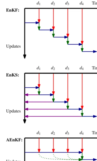
The essential difference between a smoother and a filter is that a smoother assimilates “future observations”, while a fil-ter assimilates “past observations”. This implies that for op-erational forecasting purposes, we need a filter rather than a smoother. A smoother can help improve the model accuracy in the past (e.g. for re-analysis), but it does not help improve forecast accuracy (Evensen, 2009). Therefore, Sakov et al. (2010) introduced the asynchronous ensemble Kalman filter (AEnKF), which requires forward integration of the model to obtain simulated results necessary for the analysis and model updating at the analysis step using past observations over a time window. The difference among the EnKF, EnKS and AEnKF is schematized in Fig. 1.
Sakov et al. (2010) showed that the formulation of the EnKS provides a method for asynchronous filtering, i.e. as-similating past data at once, and that the AEnKF is a gener-alization of the ensemble-based data assimilation technique. Moreover, unlike the 4-D variational assimilation methods, the AEnKF does not require any adjoint model (Sakov et al., 2010). The AEnKF is particularly attractive from an opera-tional forecasting perspective as more observations can be used with hardly any extra additional computational time. Additionally, such an approach can potentially account for a better representation of the time lag between the internal model states and the catchment response in terms of the dis-charge.
Discharge represents a widely used observation for assim-ilation into hydrological models, because it provides inte-grated catchment wetness estimates and is often available at high temporal resolution (Pauwels and De Lannoy, 2006; Teuling et al., 2010). Therefore, discharge is a popular vari-able in data assimilation studies used for model state updat-ing (e.g. Weerts and El Serafy, 2006; Vrugt and Robinson, 2007; Blöschl et al., 2008; Clark et al., 2008; Komma et al., 2008; Pauwels and De Lannoy, 2009; Noh et al., 2011a; Pauwels et al., 2013) or dual state-parameter updating (e.g Moradkhani et al., 2005b; Salamon and Feyen, 2009; Noh et al., 2011b).
The Kalman type of assimilation methods were developed for an idealized modelling framework with perfect linear problems with Gaussian statistics; however, they have been demonstrated to work well for a large number of different non-linear dynamical models (Evensen, 2009). It remains in-teresting to evaluate whether elimination of the non-linear nature of the model updating can be beneficial. For exam-ple, Xie and Zhang (2013) introduced the idea of a parti-tioned update scheme to reduce the degrees of freedom of the high-dimensional state-parameter estimation of a distributed hydrological model. In their study, the partitioned update scheme enabled them to better capture covariances between states and parameters, which prevented spurious correlations of the non-linear relations in the catchment response. Simi-larly, decreasing the number of model states being perturbed and updated was suggested by McMillan et al. (2013) to in-crease the efficiency of the filtering algorithm while
conserv-d1 d2 d3 d4 Time
d1 d2 d3 d4
Updates
d1 d2 d3 d4
EnKF:
EnKS:
AEnKF:
Updates Updates
Time
[image:2.612.326.526.66.397.2]Time
Figure 1. Illustration of the model updating procedure for the
ensemble Kalman filter (EnKF), the ensemble Kalman smoother (EnKS), and the asynchronous ensemble Kalman filter (AEnKF). The horizontal axis stands for time, observations (d1,d2,d3,d4) are
given at regular intervals. The blue arrows represent forward model integration, the red arrows denote introduction of observations and green arrows indicate model update. The magenta arrows represent the model updates for the EnKS and therefore go backward in time, as they are computed following the EnKF update every time ob-servations become available. The green dotted arrows denote past observations being assimilated using the AEnKF. The schemes for the EnKF and the EnKS are after Evensen (2009).
ing the forecast quality. Such an approach was proposed es-pecially to states with small innovations, which in their case was mainly the soil moisture storage.
obser-vations on the forecast accuracy is analysed. Secondly, the effect of a partitioned updating scheme is scrutinized.
2 Material and methods
2.1 Data and hydrological model
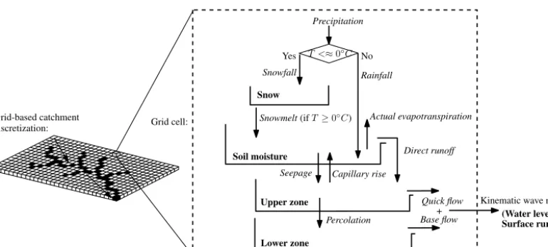
We carried out the analyses for the Upper Ourthe catchment upstream of Tabreux (area∼1600 km2, Fig. 2), which is lo-cated in the hilly region of the Belgian Ardennes, western Europe (Driessen et al., 2010). We employed a grid-based spatially distributed HBV-96 model (Hydrologiska Byråns Vattenbalansavdelning; Lindström et al., 1997), with spa-tial resolution of 1 km×1 km and hourly temporal resolu-tion. The model is forced using deterministic spatially tributed rainfall fields, which were obtained by inverse dis-tance interpolation from about 40 rain gauges measuring at an hourly time step. Evaluation of the benefits of differ-ent rainfall interpolation techniques was deemed beyond the scope of the study. We used a method used in operational practice as this study is also oriented towards operational benefits of asynchronous filtering. Additionally, there are six discharge gauges (hourly time step) situated within the catch-ment, some of which are used for discharge assimilation and some for independent validation.
For a more detailed description of the catchment and model structure and definition of the hydrological states and fluxes we refer to Rakovec et al. (2012b) and to Fig. 3. Briefly, for each grid cell the model considers the following model states: (1) snow (SN), (2) soil moisture (SM), (3) up-per zone storage (UZ) and (4) lower zone storage (LZ). The dynamics of the model states are governed by the following model fluxes: rainfall, snowfall, snowmelt, actual evapora-tion, seepage, capillary rise, direct runoff, percolaevapora-tion, quick flow and base flow. The latter two fluxes force the kinematic wave model (Chow et al., 1988; PCRaster, 2014). This rout-ing scheme calculates the overland flow usrout-ing two additional model states, the water level (H) and discharge (Q) accumu-lation over the drainage network. Model parameterization is based on the work of Booij (2002) and van Deursen (2004).
In contrast to Rakovec et al. (2012b), in the current study we employed the HBV-96 model built within a re-cently developed open-source modelling environment, Open-Streams (2014), which is suitable for integrated hydrologi-cal modelling based on the Python programming language with the PCRaster spatial processing engine (Karssenberg et al., 2009; PCRaster, 2014). The advantage of using Open-Streams (2014) is that it enables direct communication with OpenDA (2014), an open-source data assimilation toolbox. OpenDA (2014) provides a number of algorithms for model calibration and assimilation and is suitable to be connected to any kind of environmental model (e.g. Ridler et al., 2014). The import and export of hydrological and meteorological data to the system is done using Delft Flood Early
Warn-640 660 680 700 720
5520 5540 5560 5580 5600
Easting [km]
Northing [km]
●
●
●
●● ●
1
2 3
4 5 6
0 100 200 300 400 500 600 700
[image:3.612.323.528.62.214.2]Altitude [m. a.m.s.l.]
Figure 2. Topographic map of the Upper Ourthe (black line)
includ-ing the river network (blue lines), rain gauges (crosses), six river gauges (white circles labelled with numbers: 1 – Tabreux, 2 – Dur-buy, 3 – Hotton, 4 – Nisramont, 5 – Mabompré, and 6 – Ortho). Projection is in the Universal Transverse Mercator (UTM) 31N co-ordinate system. After Rakovec et al. (2012b).
ing System (Delft-FEWS, Werner et al., 2013), an open-shell system for managing forecasting processes and/or handling time series data. Delft-FEWS is a modular and highly con-figurable system, which is used by the Dutch authorities for the flood forecasting for the River Meuse basin (called RW-sOS Rivers), in which the Upper Ourthe is located. The cur-rent configuration is a stand-alone version of RWsOS Rivers; however, it can be easily switched into a configuration with real-time data import.
2.2 Data assimilation for model initialization
As stated in the introduction, we investigate the potential added value of the asynchronous EnKF (AEnKF) (Sakov et al., 2010) as compared to the traditional (synchronous) EnKF for operational flood forecasting. The derivation of the AEnKF (Sect. 2.2.2) is based on the equations using the same updating frequency (i.e. same computational costs, dif-ferent number of observations) as for the EnKF (Sect. 2.2.1), as among others presented by Rakovec et al. (2012b). 2.2.1 Ensemble Kalman filter (EnKF)
First, we define a dynamic state space system as
xk=f (xk−1,θ,uk−1)+ωk, (1)
wherexk is a state vector at timek,f is an operator
(hy-drological model) expressing the model state transition from time stepk−1 tokin response to the model input uk−1and
time-invariant model parametersθ. The noise termωk is
Snow
Soil moisture
Percolation T <≈0◦C
Precipitation
Rainfall
Upper zone
Capillary rise Seepage
Quick flow
Lower zone
Base flow+ Snowmelt(ifT≥0◦C) Actual evapotranspiration
Direct runoff
discretization: Grid cell: Grid-based catchment
Snowfall
Yes No
[image:4.612.109.494.63.236.2]Kinematic wave model (Water level, Surface runoff)
Figure 3. Left: catchment discretization using a grid-based approach including the channel delineation. Arrows indicate flow direction. Right:
schematic structure of the HBV-96 model for each grid cell. Model states are in bold and model fluxes in italics (after Rakovec et al., 2012b).
Second, we define an observation process as
yk=h (xk)+νk, (2)
where yk is an observation vector derived from the model state xk and the model parameters through the h opera-tor (in our case the kinematic wave routing model generat-ing discharge). The noise term νk is additive observational
Gaussian white noise with covariance Rk. For spatially
inde-pendent measurement errors, Rk is diagonal. Note that both
the kinematic wave routing modelh(.)and the hydrological modelf (.)exhibit non-linear behaviour.
After the model update at timek−1, the model is used to forecast model states at timek(Eq. 1). The grid-based model states form a matrix, which consists of N state vectorsxk
corresponding toN ensemble members: Xk=
x1k,x2k, . . .,xNk , (3)
where
xik=SNi1:m,SMi1:m,UZi1:m,LZi1:m, H1i:m, Qi1:mT
k. (4)
SNi, SMi, UZi, LZi,HiandQiare the HBV-96 model states of theith ensemble member (Sect. 2.1),mgives the number of grid cells andT is the transpose operator. The ensemble mean
xk=
1
N N
X
i=1
xik (5)
is used to approximate the forecast error for each ensemble member:
Ek=
x1k−xk,x2k−xk, . . .,xNk −xk
. (6)
The ensemble-estimated model covariance matrix Pk is
de-fined as
Pk=
1
N−1EkE
T
k. (7)
When observations become available, the model states of the
ith ensemble member are updated as follows:
xi,k+=xi,k−+Kk
yk−hxki,−+νik, (8) wherexi,k+is the analysis (posterior, or update) model state matrix andxi,k−is the forecast (prior) model state matrix. Kk
is the Kalman gain, a weighting factor of the errors in model and observations:
Kk=PkHTk
HkPkHTk +Rk
−1
, (9)
where PkHTk is approximated by the forecasted covariance
between the model states and the forecasted discharge at the observing locations, and HkPkHTk is approximated by the
covariance of forecasted discharge at the observing locations (Houtekamer and Mitchell, 2001):
PkHTk =
1
N−1
N
X
i=1
xik−xk hxik−h (xk) T
, (10)
HkPkHTk =
1
N−1
N
X
i=1
hxik−h (xk) h
xik−h (xk)
T
, (11) where
h (xk)=
1
N N
X
i=1
hxik. (12)
(Sect. 2.2.1) using a state augmentation approach. This means that theith vector of model states (xik) at timek(see Eq. 4) is augmented with the past forecasted observations
h(xik−1), . . . ,h(xik−W)(i.e. model outputs corresponding to the observation locations) fromWprevious time steps, which yields
ex
i k=
xik
h xik−1
h xik−2 .. . h xik−W
. (13)
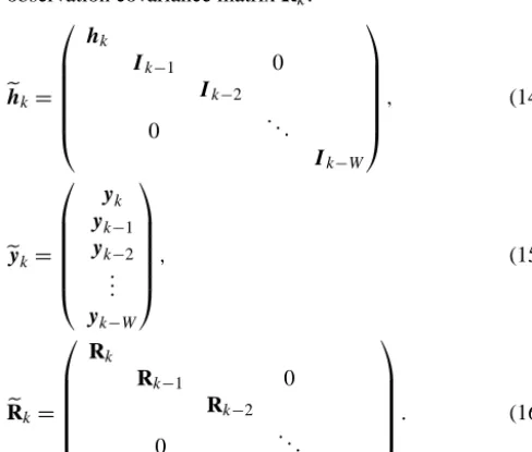
Remember that the size ofxikandh(xik−1), . . . ,h(xik−W)can significantly differ: xik contains the complete set of model states, whileh(xik−1), . . . ,h(xik−W)contains only the fore-casted observations. Additionally, with the new state defini-tion comes a new augmented observer operatorehk(in which
I, with the corresponding subscript, stands for identity ele-ments on the diagonal, matching the dimensions in Eq. 13), a new augmented observation vectoreyk and its corresponding observation covariance matrixeRk:
ehk=
hk
Ik−1 0
Ik−2
0 . ..
Ik−W
, (14)
eyk=
yk yk−1
yk−2 .. .
yk−W
, (15)
e
Rk=
Rk
Rk−1 0
Rk−2
0 . ..
Rk−W
. (16)
Having these augmented equations forexik,ehk,eykandeRk, it is
straightforward to carry out the assimilation in the same man-ner as presented in Sect. 2.2.1. Note that although current and past observations are used to construct the augmented state vector in Eq. (13), in practice Eq. (8) is solved only to the current stateexik (i.e. the indices that correspond toxik) and the rest is ignored. The presence of past observation terms increases the dimension ofePk andeKk (see Eqs. 7 and 9) in
both directions (rows and columns). Each column ofKek
cor-responds to an observation. The extra column ofeKk
corre-sponds to the past observations. Hence, it is possible to sim-ply solve the equations for the first rows, which correspond only toxik. Note that the first rows ofeKkalso contain the
[image:5.612.45.289.337.544.2]con-tributions of the past observations to the current state. These
Table 1. Overview of the periods used in this study.
Period Number of Maximum observed events discharge[m3s−1]
23 Oct 1998–15 Nov 1998 1 210 15 Feb 1999–05 Mar 1999 2 195 15 Jan 2002–06 Mar 2002 4 340 21 Dec 2002–07 Jan 2003 1 380
contributions arise from the off-diagonal terms of the aug-mented covarianceePk. Finally, if the time window equals the
current single time step, thenW=0 and the AEnKF problem reduces to the traditional EnKF.
From the operational point of view, it is preferable to have a longer assimilation window, because less frequent assimi-lation eliminates a disruption of the ensemble integration by an update and a restart. When assimilation is done more fre-quently, it will cause considerably higher calculation costs, which can often be a burden for real-time operational settings (Sakov et al., 2010). The AEnKF uses a longer assimilation window and assimilates all observations in a single update. This makes the AEnKF attractive for operational use. The added value of a longer assimilation window will be a sub-ject for investigation in this work. Especially, it can provide an improved representation of the time lag between the inter-nal model states and the catchment response in terms of the discharge. Such an idea was investigated for example by Li et al. (2013), who compared the effect of time-lag represen-tation using the EnKF and EnKS.
2.3 Model uncertainty
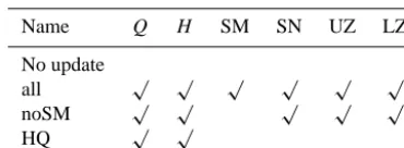
Table 2. Four partitioned state updating schemes (indicated in
the first column) for five model states (indicated in the first row) being updated and thus included in the model analysis. Model states are described in Sect. 2.1 and Fig. 3 and have the follow-ing acronyms: discharge (Q), water level (H), soil moisture stor-age (SM), snow storstor-age (SN), upper zone storstor-age (UZ), and lower zone storage (LZ).
Name Q H SM SN UZ LZ
No update
all √ √ √ √ √ √
noSM √ √ √ √ √
HQ √ √
DA using complex spatially distributed hydrological models see Noh et al. (2014).
2.4 Experimental setup
This section provides a configuration setup of the filtering methods (Sect. 2.2.1 and 2.2.2) to assimilate discharge ob-servations into a spatially distributed hydrological model of the Upper Ourthe catchment. The objective is to improve the hydrological forecast at the catchment outlet (at Tabreux, gauge 1 in Fig. 2) by assimilating up to four discharge gauges, numbered as 1, 3, 5, 6 in Fig. 2. Note that discharge data from multiple gauges are assimilated simultaneously and no localization is employed in this study. Additionally, validation at an independent location is also performed. The discharge assimilation is performed every 24 h; however, the forecasts are issued every 6 h, i.e. 4 times a day, with differ-ent independdiffer-ent starting points at 00:00, 06:00, 12:00, and 18:00 UTC, which is the same implementation as used by Rakovec et al. (2012b). This study analyses the eight largest flood peaks observed within the catchment since 1998. An overview is provided in Table 1.
The ensemble of uncertain model simulations is obtained by perturbing the SM state with the spatio-temporally cor-related error model (Sect. 2.3). With this approach we en-sured that the error model produced reasonable results in the open loop and did not lead to any numerical instability. More complex ways of perturbing the model and their effects on forecast accuracy were studied before (see Rakovec et al., 2012a; Noh et al., 2014) and were deemed beyond the scope of this manuscript. The ensemble size in this study was de-fined to be 36 realizations (for computational reasons). Note that increased ensemble sizes of 72 and 144 realizations did not influence the results (not shown). Nevertheless, such a small ensemble size as presented in the manuscript would not be possible if parameter estimation would be involved or if more complex error models would be employed. The error in the discharge observations is considered to be a normally distributed observation error with a variance of (0.1Qobs,k)2
(after e.g. Weerts and El Serafy, 2006; Clark et al., 2008).
Dischar
ge [
m
3
s
−
1
]
0
50
100
150
●
●●● ●
●● ● ● ● ● ● ● gauge 1
●
● ● ● ● ● ● ● ● ●● ●● gauge 3
Time [h]
29Dec02
31Dec02
0
50
100
150
●
● ● ● ● ● ● ●● ● ● ● ● gauge 5
29Dec02
31Dec02
●
[image:6.612.74.259.152.220.2]● ● ● ● ● ● ●● ● ● ● ● gauge 6
Figure 4. Discharge ensemble forecasts (grey lines) and
observa-tions (points) at four locaobserva-tions (gauges 1, 3, 5, 6; see Fig. 2). Obser-vations being assimilated using the AEnKF are schematized accord-ing to the state augmentation size for two scenarios: assimilation of data from the current time stepW=0 (open circle, traditional EnKF approach) and assimilation of data including the previous 11 time steps,W=11 (black dots). The observations are assimilated into the model states on 31 December 2002, 00:00 UTC.
The experimental setup scrutinizes the problem of asyn-chronous filtering from two perspectives. First, we investi-gate the effect of state augmentation using the past obser-vations and assimilation of distributed obserobser-vations on the state innovation (Sect. 3.1). Recall that the number of ob-servations being assimilated into the model depends on the magnitude of W. Furthermore, the choice of which model states are included in the analysis step to be updated is anal-ysed (Sects. 3.2, and 3.3). This means that besides updating all of the model states, we will test two other alternatives. The first alternative will leave out from the model analysis the soil moisture state (noSM), which is known to exhibit the most non-linear relation to Q. The second alternative will eliminate all the model states except for the two rout-ing ones (HQ). The scenarios of the partitioned state updat-ing schemes are shown in Table 2, includupdat-ing the control run without state updating (no update).
er-rors in the same units as the variable. The perfect forecast in terms of the ROC and BS scores has a value of 1 and values smaller than 1 indicate forecast deterioration.
3 Results
3.1 The effect of state augmentation and distributed observations on state innovation
[image:7.612.310.545.62.316.2]To investigate and understand the effect of augmented op-erators (Eqs. 13, 14, and 15) on the innovation of spatially distributed model states, we present the following example. Figure 4 shows discharge simulations and corresponding dis-charge observations at four locations within the catchment on 31 December 2002, 00:00 UTC. Note that the magnitude of the discharge observations is a function of the location within the catchment; for downstream gauges the magnitude is larger than for the more upstream gauges. The discharge observations are further distinguished according to the time-window length of the state augmentation, which is set to
W=0 and W=11. The first example represents the tradi-tional EnKF algorithm, while the latter assimilates observa-tions from a 12 h time window (i.e. 1 current observation and 11 past observations), which is arbitrarily defined as half the 24 h assimilation time window. For some cases alternative as-similation windows were tested, which did not lead to notice-able differences however (not shown). Note that the amount of information being assimilated into the model differs for different values ofW.
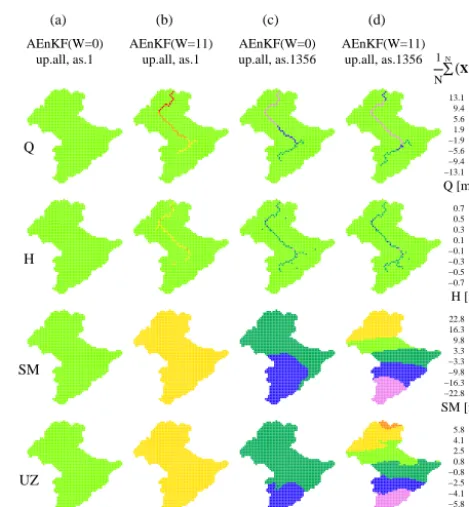
The mean difference between the forecasted and updated model states for the whole ensemble is illustrated in Fig. 5 for four scenarios. These examples improve our understand-ing about the behaviour of the updated model states in rela-tion to the informarela-tion content of the observarela-tions from two perspectives: (1) the effect of assimilating also past obser-vations in addition to obserobser-vations at the current (analysis) time, and (2) the effect of assimilating spatially distributed observations into a grid-based hydrological model.
Let us first consider the traditional EnKF (i.e. no state aug-mentation with W=0) to update all the grid-based model states by assimilating the observation at the catchment outlet (gauge 1). We observe that the single observation is mea-sured approximately in the middle of the simulated ensem-ble (see the open circle for gauge 1 in Fig. 4). Therefore, there is hardly any difference between the forecasted and updated model states as we show in Fig. 5a. In the sec-ond scenario, we still assimilate only one gauge at the out-let; however, we use the augmented operators withW=11. Because the mean of the ensemble simulations is predom-inantly underestimated as compared to the assimilated ob-servations (see black dots in Fig. 4 for gauge 1), after the update more water is added spatially equally into the sys-tem, as shown in Fig. 5b. In the third scenario, we include all four gauges being assimilated into the model without any
Q
H
SM
UZ
−13.1 −9.4 −5.6 −1.9 1.9 5.6 9.4 13.1
Q [m3/s]
−0.7 −0.5 −0.3 −0.1 0.1 0.3 0.5 0.7
H [m]
−22.8 −16.3 −9.8 −3.3 3.3 9.8 16.3 22.8
SM [mm]
−5.8 −4.1 −2.5 −0.8 0.8 2.5 4.1 5.8
UZ [mm]
1 N∑
N (X−
−X+)
:
(a) (b) (c) (d)
AEnKF(W=0) AEnKF(W=11) AEnKF(W=0) AEnKF(W=11) up.all, as.1 up.all, as.1 up.all, as.1356 up.all, as.1356
Figure 5. Mean difference between the forecasted (X−) and up-dated (X+) model states on 31 December 2002 at 00:00 UTC for different scenarios (shown in vertical panels). We show only four sensitive model states: discharge (Q), water level (H), soil mois-ture (SM) and upper zone (UZ). We excluded the insensitive lower zone (LZ). NotationsW=0 andW=11 indicate the size of the state augmentation. Notation up.all indicates that all of the model states are updated. Notation as “xx” indicates the gauges which are assimilated; see Fig. 2 for their locations. The corresponding en-semble of model forecasts and observations being assimilated are shown in Fig. 4.
augmentation. Because the model simulations at the interior gauges are mostly overestimating the observations, water is removed from the catchment during the update. Moreover, since the model overestimation is largest at gauges 3 and 6, we can also observe in Fig. 5c how well the EnKF is ca-pable of identifying corresponding regions in a spatial man-ner. In the fourth scenario (Fig. 5d) we still assimilate all four gauges; however, we augment the state withW=11. We can observe that the innovation of the model states gets even more spatially differentiated; the updated SM and UZ model states in the downstream part of the catchment increase the amount of water in the system, while the updated SM and UZ model states in the upstream part decrease the amount of water in the system.
Figure 6. Ensemble of discharge forecasts for a typical event at the catchment outlet (Tabreux, gauge 1) for three updating scenarios: all,
noSM, and HQ (see Table 2 for definition). The combined effect of the model states being updated (three scenarios shown in rows) and the length of the state augmentation vector (W) of past observations being assimilated (two scenarios in columns) is presented. Gauges 1, 3, 5, and 6 are assimilated. The control run (with no update) is shown in the left panel. The observations are shown in black.
3.2 The effect of the four partitioned update schemes and asynchronous assimilation on forecast accuracy
We present a qualitative interpretation of the hydrological forecasts with a lead time of 48 h in Fig. 6 for different parti-tioned state updating schemes as defined in Table 2, includ-ing both a non-augmented state (W=0) and an augmented state (W=11). This analysis focuses on a characteristic win-ter flood event (December 2002–January 2003) being typical for a moderate temperate climate caused by a fast-moving frontal stratiform system (Hazenberg et al., 2011). We ob-serve that the ensemble of the control runs (top panel of Fig. 6) simulates the major flood peak reasonably well, in-cluding the timing and the magnitude; however, it has a larger spread with respect to the assimilation scenarios. Addition-ally, when we consider the ensemble mean of the no-update scenario with respect to the assimilation scenarios, the accu-racy deteriorates. When discharge assimilation is employed, an overall reduction of the uncertainty in the forecasted en-semble is observed. Nevertheless, the forecasted flood peak becomes underestimated and the forecasted recession re-mains overestimated, which is acceptable because of the de-fined uncertainty in the observed discharge. This happens in particular for the scenario in which all states are updated; there are marginal differences between the non-augmented and augmented model states. Furthermore, when we leave
out SM from the state update (noSM), we can observe that the major flood peak is forecasted more accurately, includ-ing the risinclud-ing limb around 31 December 2002. Moreover, for the augmented state withW=11, the ensemble spread be-comes somewhat wider for lead times exceeding 12 h than for the non-augmented state. Nevertheless, the observations correspond approximately with the ensemble mean. Finally, we present the effect of the scenario in which only the two routing states are updated. The results suggest that the flood peak is captured most accurately of all scenarios, however with somewhat wider uncertainty bands. Therefore, it seems more appropriate to exclude the UZ storage (noSM scenario) in the model state updating, which represents water storage available for quick catchment response in the concept of the HBV model.
(a)
(b)
10 15 20 25 30 35Lead time [h]
RMSE [ m 3 s − 1 ] ● ●● ● ● ● ●● ● ● ●● ●● ● ●● ●● ●● ● ● ● ●● ● ● ●● ●● ● ● ● ● ●● ● ● ● ● ● ●● ● ● ● ● ●● ● ● ●● ●● ●● ● ●● ● ●● ● ●● ● ●● ● ●●● ● ● ●● ●● ● ●● ●● ● ● ● ● ●● ● ● ● ● ●● ●● ●● ●● ●● ●● ●● ●● ●● ●● ●● ● ●● ●● ● ●● ● ●● ●● ● ● ● ● ●● ● ● ● ●● ● ●
0 5 10 15 20 25 30 35 40 45
● Update: no update all noSM HQ ● Augmentation W: 0 5 11 0.5 0.6 0.7 0.8 0.9 1.0
Lead time [h]
R OC [−] ● ● ● ● ● ● ●●● ● ●● ● ● ● ●● ● ●●● ● ● ● ●●● ● ● ● ●● ● ● ● ●● ● ●● ●● ● ● ● ● ● ● ●● ● ● ● ● ● ●● ●● ● ● ● ● ● ● ● ●●● ●●● ● ● ● ● ● ● ●●● ● ● ● ● ● ● ● ● ●● ● ● ● ● ● ● ● ●● ●● ● ● ●● ● ● ● ● ● ● ● ●●●● ● ● ● ●●● ● ●● ● ● ● ● ●●● ● ● ● ● ●● ● ● ● ● ●
0 5 10 15 20 25 30 35 40 45
● Update: no update all noSM HQ ● Augmentation W: 0 11
(c)
(d)
0.0 0.2 0.4 0.6 0.8Lead time [h]
BSS [−] ● ● ● ● ● ● ● ● ●●● ● ●● ● ● ●●●● ● ● ● ●● ● ● ● ● ● ● ● ● ● ● ● ● ● ● ● ● ● ●● ● ● ● ● ● ● ●●●● ● ● ● ● ●● ● ● ●● ● ● ● ● ● ● ● ● ● ● ● ● ●● ● ● ● ● ● ● ●●● ● ● ●● ●●● ● ● ● ● ● ● ● ● ● ●● ● ● ● ●● ● ● ● ●● ● ● ● ● ● ● ● ● ● ● ● ●● ● ● ● ● ● ●● ● ● ● ●● ● ● ● ●
0 5 10 15 20 25 30 35 40 45
● Update: no update all noSM HQ ● Augmentation W: 0 11 10 15 20 25
Lead time [h]
RMSE [ m 3 s − 1 ] ●● ● ● ● ●● ● ●● ● ● ●●● ● ● ● ●● ● ●● ● ●● ●● ● ● ● ●● ● ● ● ● ●● ● ● ● ● ● ● ● ● ● ● ●● ● ● ●● ●● ●● ●● ●●●● ●● ●●● ● ●●● ● ●● ●● ● ●● ● ●● ● ● ● ●● ● ● ● ● ● ● ●● ● ●● ●● ●● ●● ● ● ● ●● ●● ● ●● ●● ●● ●● ●● ●● ● ● ● ●● ● ● ● ● ● ● ● ●● ● ● ●
0 5 10 15 20 25 30 35 40 45
● Update: no update all noSM HQ ● Augmentation W: 0 5 11
0.0
0.2
0.4
0.6
0.8
Lead time [h]
BSS [−]
● ● ● ● ● ● ● ● ●●● ● ●● ● ● ●● ● ● ● ● ● ●● ● ● ● ● ● ● ● ● ● ● ● ● ● ● ● ● ● ●●● ● ● ● ● ● ●●●● ● ●●●●● ● ● ●● ● ● ● ● ● ● ● ● ● ● ● ● ●● ● ●● ● ● ● ●●● ● ● ●● ●●● ● ● ● ● ● ● ● ● ● ●● ● ● ● ●● ● ● ● ●● ● ● ● ● ● ● ● ● ● ● ● ●●● ● ● ● ● ● ● ● ● ● ●● ● ● ● ●0
5
10
15
20
25
30
35
40
45
●
Update:
no update
all
noSM
HQ
●Augmentation W:
0
11
10
15
20
25
30
35
Lead time [h]
RMSE [
m
3
s
−
1
]
0
5
10
15
20
25
30
35
40
45
●
Update:
no update
all
noSM
HQ
●Augmentation W:
0
5
11
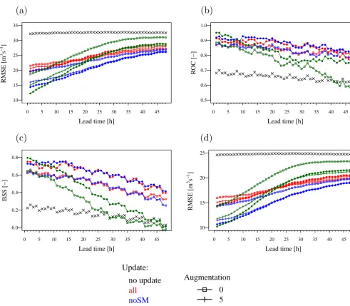
Figure 7. (a) Root-mean-square error (RMSE), (b) relative operating characteristic (ROC), and (c) Brier skill score (BSS) at Tabreux
(gauge 1) for different discharge observation vectors for which different model states are updated and with different lengths of the state augmentation vector (W) of past observations being assimilated. The results incorporate a set of eight flood events shown in Table 1. Gauges 1, 3, 5, and 6 are assimilated. For BSS, the reference forecast is the sample climatology and only values larger than the 25th percentile of the whole sample are considered. (d) Same as (a) but the results are presented for Durbuy (gauge 2), a validation location which is not assimilated.
Figure 7a shows the RMSE as a function of lead time for different partitioned state updating schemes and for three scenarios for the state augmentation at the catchment out-let (Tabreux). The control model run with no update has a constant RMSE of about 32 m3s−1 and an improved
hy-drological forecast has a RMSE lower than the control run. The results suggest that all assimilation scenarios improve the hydrological forecast, however, with marked differences between the scenarios. Figure 7a also clearly shows that the differences in the forecast improvement of these vari-ous setups are purely due to using multiple data points in
[image:9.612.53.545.62.491.2]2920 O. Rakovec et al.: Asynchronous filtering for flood forecasting (a) −30 −20 −10 0 10 20 21Dec02 04Jan03 −30 −20 −10 0 10 20 Normalized dif
ference in Q [%]
−30 −20 −10 0 10 20 −30 −20 −10 0 10 20 −30 −20 −10 0 −30 −20 −10 0 10 20 21Dec02 04Jan03 −30 −20 −10 0 10 20 Normalized dif
ference in H [%]
−30 −20 −10 0 10 20 −30 −20 −10 0 10 20 −30 −20 −10 0 −30 −20 −10 0 10 20 Time [h] 21Dec02 04Jan03 −30 −20 −10 0 10 20 Normalized dif
ference in SM [%]
−30 −20 −10 0 10 20 −30 −20 −10 0 10 20 −30 −20 −10 0 −30 −20 −10 0 10 20 21Dec02 04Jan03 −30 −20 −10 0 10 20 Normalized dif
ference in UZ [%]
−30 −20 −10 0 10 20 −30 −20 −10 0 10 20 −30 −20 −10 0 −0.10 −0.05 0.00 0.05 0.10 21Dec02 04Jan03 −0.10 −0.05 0.00 0.05 0.10 −0.10 −0.05 0.00 0.05 0.10 −0.10 −0.05 0.00 0.05 0.10 −0.10 −0.05 0.00 ● 1 3 6 5 HQ noSM all no update no update −no update
(b) −30 −20 −10 0 10 20 21Dec02 04Jan03 −30 −20 −10 0 10 20 Normalized dif
ference in Q [%]
−30 −20 −10 0 10 20 −30 −20 −10 0 10 20 −30 −20 −10 0 10 20 −30 −20 −10 0 10 20 21Dec02 04Jan03 −30 −20 −10 0 10 20 Normalized dif
ference in H [%]
−30 −20 −10 0 10 20 −30 −20 −10 0 10 20 −30 −20 −10 0 10 20 −30 −20 −10 0 10 20 Time [h] 21Dec02 04Jan03 −30 −20 −10 0 10 20 Normalized dif
ference in SM [%]
−30 −20 −10 0 10 20 −30 −20 −10 0 10 20 −30 −20 −10 0 10 20 −30 −20 −10 0 10 20 21Dec02 04Jan03 −30 −20 −10 0 10 20 Normalized dif
ference in UZ [%]
−30 −20 −10 0 10 20 −30 −20 −10 0 10 20 −30 −20 −10 0 10 20 −0.10 −0.05 0.00 0.05 0.10 21Dec02 04Jan03 −0.10 −0.05 0.00 0.05 0.10 −0.10 −0.05 0.00 0.05 0.10 −0.10 −0.05 0.00 0.05 0.10 −0.10 −0.05 0.00 0.05 0.10 ● Location: 1 3 6 5 HQ noSM all no update no update −no update
Location: 1 3
[image:10.612.128.466.65.460.2]6 5
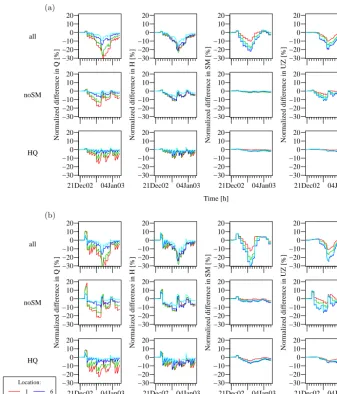
Figure 8. Scaled difference between the ensemble mean for the three partitioned update schemes and the control run without data assimilation
at four gauging locations (shown by different colours) within the Upper Ourthe catchment using the AEnKF with (a)W=0 and (b)W=11. We excluded the insensitive lower zone (LZ). Gauges 1, 3, 5, and 6 are assimilated. The results correspond to the same period as presented in Fig. 6.
the improved effect does not last as long as for the noSM scenario. The smallest improvement at shorter lead times is achieved when all model states are updated (scenario all). This is due to the strongly non-linear relation between the as-similated observations and the SM storage, which is further articulated by the time lag between the state and the catch-ment response. Nevertheless, for longer lead times it seems slightly better to update all states rather than only the rout-ing states. Discharge is related to the SM and UZ storages through the Kalman gain. When the correlation is lower the update will be smaller. AEnKF exploits the correlation be-tween the present discharge state and the discharge state not only at the previous time step but also further in the past. It may be possible to use the correlation between discharge at the present time and UZ/SM in the past for data
assimila-tion; however, this is deemed beyond the scope of this study. Nevertheless, we speculate that this will only be useful in a smoothing context (i.e. the present discharge may bring in-formation on UZ/SM in the past), not in a filtering context as in the present study.
Validation of the model setup in terms of the RMSE is pre-sented in Fig. 7d for an independent evaluation of the fore-casting results at Durbuy, an interior location which was not used for assimilation. These results show that an improve-ment of discharge assimilation also occurs at the validation location and that the pattern corresponds well to the results presented in Fig. 7a. Such an analysis indicates that there is no spurious update of the model states.
ver-ification measures: the ROC score and the BS score (see Fig. 7b and c). Recall that values of 1 represent a perfect forecast, while values smaller than 1 indicate forecast deteri-oration. Similar to the RMSE results, updating only the two routing states (HQ) is most efficient for short lead times, but this skill disappears quickly for longer lead times. In terms of the ROC and BS scores, for a given augmentation size, there are marginal differences between the scenarios which update all states (all) and which leave the soil moisture out (noSM). However, it is notable that the state augmentation case (W=11) improves the forecast performance as com-pared to the no augmentation case (W=0). Note that the state augmentation ofW=5 was not carried out.
3.3 Temporal nature of model state innovations
To reveal the temporal nature of the model being updated using the AEnKF, usingW=0 andW=11, we present in Fig. 8a and b time series of normalized differences between the ensemble means for the three partitioned update schemes and the ensemble mean for the no-update scenario. The nor-malization is achieved by dividing the aforementioned dif-ference by the no-update scenario mean. In such a way we obtain the relative change in each of the model states. For the AEnKF usingW=0 (Fig. 8a), we can observe that for the scenario “all”, which updates all the model states, the magni-tude of the percentage change is approximately the same for all four model states and ranges up to 25 %. When all model states except for the SM are updated, no changes in the SM storage occur and the overall magnitude of the changes in the other states is slightly decreased and smoothed. Furthermore, when only the two routing states are updated (HQ), the SM and UZ storages remain constant over time and we observe a different temporal behaviour of the routing states in com-parison with the previous cases. For the HQ scenario, the up-dated time series have a clear zigzag shape, which indicates that the effect of updating diminishes faster because only the river channel is updated. In contrast, the routing states for the other cases show a more stable behaviour over time, il-lustrated by the stepwise shape. These more persistent results correspond to the updates in the UZ storage, which is used for a quick catchment response and has an impact for a longer time. The benefits of including the UZ storage in the update and leaving the SM storage out was already presented from a different point of view in Fig. 7a for longer lead times.
For the AEnKF usingW=11 (Fig. 8b), we can observe that the overall pattern of the temporal changes in the model states is similar as for W=0, but the behaviour of using
W=11 shows somewhat larger variability. By assimilating more observations (W=11), we expect an even larger up-date, assuming that more observations contain more infor-mation about the unknown truth. Assuming the underlying forecast model has a significant error, by assimilating more observations the Kalman filter will pull the model even closer to the truth, yielding a larger abrupt update.
4 Conclusions
We applied the asynchronous ensemble Kalman filter (AEnKF) (Sakov et al., 2010) and identified the effect of augmenting the state vector with past simulations and ob-servations. To our knowledge this is the first application of the AEnKF in flood forecasting. We showed that the ef-fect of an augmented assimilation vector improves the flood forecasts, but the contribution gets smaller for longer lead times. Overall, the AEnKF can be considered as an effective method for model state updating taking into account more (e.g. all) observations at hardly any additional computational burden. This makes it very suitable for operational hydro-logical forecasting. When compared to standard EnKF, the AEnKF allows for the choice of a certain assimilation win-dow length, which adds a degree of freedom to the data as-similation scheme. The optimal window is very likely re-lated to the catchment size (i.e. concentration time). It was noted (not shown) that for the smaller upstream catchments the optimal window was smaller than for the complete Upper Ourthe catchment, although there was no negative effect of a longer assimilation window (W=5 vs.W=11). For the high flows analysed in this study, the AEnKF with a longer time windowW is able to make corrections that last longer on average than with the shorter time windowW. Character-ization of the statistical properties of the temporal flow dy-namics (i.e. typical timescales of flood peaks as compared to low flows) is however a relevant issue. The length of the time windowWhas to be seen relative to the timescale of the river flow dynamics. We assume that for low flow conditions, the improved skill of longerWwith respect to shorterWwill be-come negligible, as low flows exhibit less temporal dynam-ics than high flows. We refer to Pan and Wood (2013) for an analysis about explicit handling of lags in space and time, which uses a state augmentation approach for a linear inverse streamflow routing model. Note that it was not the objective of this study to determine the optimal assimilation window for the AEnKF given various river flow dynamics. Another limitation of this study is the relatively simple error model for perturbing only soil moisture states. More complex ways of perturbing the model and their effects on forecast accuracy deserve more attention in future studies.
hand, it was recently demonstrated that a rainfall–runoff model can be improved when constrained by remotely sensed soil moisture (e.g. Alvarez-Garreton et al., 2014; Wanders et al., 2014a, b) or in situ soil moisture (e.g. Lee et al., 2011). Moreover, we showed that keeping the quick catchment re-sponse storage (upper zone; UZ) in the model analysis is im-portant, especially for longer lead times, when compared to the scenario in which only two routing storages were up-dated. The UZ seems to compensate the effect of SM on discharge. The fact that excluding SM extends the improve-ments suggests that in our case the discharge forecasts with a lead time of 2 days (and for major flood events) are less de-pendent on SM. A possible alternative to excluding the SM storage from the analysis would be to investigate the use of other algorithms, for example the maximum likelihood en-semble filter (MLEF) (Zupanski, 2005; Rafieeinasab et al., 2014), which is more suited for use with highly non-linear observation operators.
Acknowledgements. We would like to thank Arno Kockx and
Martin Verlaan for their help with the OpenDA configuration and Jaap Schellekens for help with the OpenStreams configuration (all from Deltares). We thank Paul Torfs (Wageningen University), Seong Jin Noh (KICT, Korea), Ming Pan (Princeton University), two anonymous reviewers and the editor for their comments on the manuscript. This project is financially supported by the Flood Control 2015 program (http://www.floodcontrol2015.nl), which is gratefully acknowledged. We thank the Hydrological Service of the Walloon Region of Belgium (MET-SETHY) and the Royal Meteorological Institute of Belgium (KMI) for providing the hydrological and meteorological data.
Edited by: N. Verhoest
References
Alvarez-Garreton, C., Ryu, D., Western, A., Crow, W., and Robert-son, D.: The impacts of assimilating satellite soil moisture into a rainfall-runoff model in a semi-arid catchment, J. Hydrol., 519, 2763–2774, doi:10.1016/j.jhydrol.2014.07.041, 2014.
Blöschl, G., Reszler, C. R., and Komma, J.: A spatially distributed flash flood forecasting model, Environ. Model. Softw., 23, 464– 478, 2008.
Booij, M.: Appropriate modelling of climate change impacts on river flooding, PhD thesis, University of Twente, Enschede, the Netherlands, 2002.
Brown, J. D. and Seo, D.-J.: Evaluation of a nonparamet-ric post-processor for bias correction and uncertainty estima-tion of hydrologic predicestima-tions, Hydrol. Process., 27, 83–105, doi:10.1002/hyp.9263, 2013.
Brown, J. D., Demargne, J., Seo, D.-J., and Liu, Y.: The Ensem-ble Verification System (EVS): A software tool for verifying ensemble forecasts of hydrometeorological and hydrologic vari-ables at discrete locations, Environ. Model. Softw., 25, 854–872, doi:10.1016/j.envsoft.2010.01.009, 2010.
Chow, V. T., Maidment, D., and Mays, L.: Applied Hydrology, McGraw-Hill, New York, USA, 1988.
Clark, M. P., Rupp, D. E., Woods, R. A., Zheng, X., Ib-bitt, R. P., Slater, A. G., Schmidt, J., and Uddstrom, M. J.: Hydrological data assimilation with the ensemble Kalman fil-ter: Use of streamflow observations to update states in a dis-tributed hydrological model, Adv. Water Resour., 31, 1309– 1324, doi:10.1016/j.advwatres.2008.06.005, 2008.
Crow, W. T. and Ryu, D.: A new data assimilation approach for improving runoff prediction using remotely-sensed soil moisture retrievals, Hydrol. Earth Syst. Sci., 13, 1–16, doi:10.5194/hess-13-1-2009, 2009.
Driessen, T. L. A., Hurkmans, R. T. W. L., Terink, W., Hazen-berg, P., Torfs, P. J. J. F., and Uijlenhoet, R.: The hydrological response of the Ourthe catchment to climate change as mod-elled by the HBV model, Hydrol. Earth Syst. Sci., 14, 651–665, doi:10.5194/hess-14-651-2010, 2010.
Dunne, S. and Entekhabi, D.: Land surface state and flux estima-tion using the ensemble Kalman smoother during the Southern Great Plains 1997 field experiment, Water Resour. Res., 42, 1– 15, doi:10.1029/2005WR004334, 2006.
Evensen, G.: Sequential data assimilation with a nonlinear quasi-geostrophic model using Monte Carlo methods to forecast error statistics, J. Geophys. Res., 99, 10143–10162, 1994.
Evensen, G.: The Ensemble Kalman Filter: theoretical formula-tion and practical implementaformula-tion, Ocean Dynam., 53, 343–367, 2003.
Evensen, G.: Data Assimilation: The Ensemble Kalman Filter, Springer, Berlin, Heidelberg, Germany, doi:10.1007/978-3-642-03711-5, 2009.
Evensen, G. and Van Leeuwen, P.: An ensemble Kalman smoother for nonlinear dynamics, Mon. Weather Rev., 128, 1852–1867, 2000.
Hazenberg, P., Leijnse, H., and Uijlenhoet, R.: Radar rain-fall estimation of stratiform winter precipitation in the Belgian Ardennes, Water Resour. Res., 47, 1–15, doi:10.1029/2010WR009068, 2011.
Houtekamer, P. L. and Mitchell, H. L.: A sequential ensemble Kalman filter for atmospheric data assimilation, Mon. Weather Rev., 129, 123–137, 2001.
Karssenberg, D., Schmitz, O., Salamon, P., De Jong, C., and Bierkens, M. F. P.: A software framework for con-struction of process-based stochastic spatio-temporal mod-els and data assimilation, Environ. Model. Softw., 25, 1–14, doi:10.1016/j.envsoft.2009.10.004, 2009.
Komma, J., Blöschl, G., and Reszler, C.: Soil moisture updating by ensemble Kalman filtering in real-time flood forecasting, J. Hy-drol., 357, 228–242, doi:10.1016/j.jhydrol.2008.05.020, 2008. Lee, H., Seo, D.-J., and Koren, V.: Assimilation of streamflow
and in situ soil moisture data into operational distributed hy-drologic models: Effects of uncertainties in the data and initial model soil moisture states, Adv. Water Resour., 34, 1597–1615, doi:10.1016/j.advwatres.2011.08.012, 2011.
Lindström, G., Johansson, B., Persson, M., Gardelin, M., and Bergström, S.: Development and test of the distributed HBV-96 hydrological model, J. Hydrol., 201, 272–288, 1997.
Liu, Y. and Gupta, H. V.: Uncertainty in hydrologic modeling: To-ward an integrated data assimilation framework, Water Resour. Res., 43, 1–19, doi:10.1029/2006WR005756, 2007.
Liu, Y., Weerts, A. H., Clark, M., Hendricks Franssen, H.-J., Kumar, S., Moradkhani, H., Seo, D.-J., Schwanenberg, D., Smith, P., van Dijk, A. I. J. M., van Velzen, N., He, M., Lee, H., Noh, S. J., Rakovec, O., and Restrepo, P.: Advancing data assimilation in operational hydrologic forecasting: progresses, challenges, and emerging opportunities, Hydrol. Earth Syst. Sci., 16, 3863–3887, doi:10.5194/hess-16-3863-2012, 2012.
McMillan, H. K., Hreinsson, E. O., Clark, M. P., Singh, S. K., Za-mmit, C., and Uddstrom, M. J.: Operational hydrological data assimilation with the recursive ensemble Kalman filter, Hydrol. Earth Syst. Sci., 17, 21–38, doi:10.5194/hess-17-21-2013, 2013. Moore, R. J.: The PDM rainfall-runoff model, Hydrol. Earth Syst.
Sci., 11, 483–499, doi:10.5194/hess-11-483-2007, 2007. Moradkhani, H., Hsu, K. L., Gupta, H., and Sorooshian, S.:
Uncer-tainty assessment of hydrologic model states and parameters: Se-quential data assimilation using the particle filter, Water Resour. Res., 41, 1–17, 2005a.
Moradkhani, H., Sorooshian, S., Gupta, H., and Houser, P. R.: Dual state-parameter estimation of hydrological models using ensem-ble Kalman filter, Adv. Water Resour., 28, 135–147, 2005b. Noh, S., Tachikawa, Y., Shiiba, M., and Kim, S.: Applying
se-quential Monte Carlo methods into a distributed hydrologic model: Lagged particle filtering approach with regularization, Hydrol. Earth Syst. Sci., 15, 3237–3251, doi:10.5194/hess-15-3237-2011, 2011a.
Noh, S. J., Tachikawa, Y., Shiiba, M., and Kim, S.: Dual state-parameter updating scheme on a conceptual hydrologic model using sequential Monte Carlo filters, J. Jpn. Soc. Civ. Eng. Ser. B1, 67, I1–I6, 2011b.
Noh, S. J., Rakovec, O., Weerts, A. H., and Tachikawa, Y.: On noise specification in data assimilation schemes for improved flood forecasting using distributed hydrological models, J. Hy-drol., 519, 2707–2721, doi:10.1016/j.jhydrol.2014.07.049, 2014. OpenDA: The OpenDA data-assimilation toolbox, http://www.
openda.org, last access: 1 November 2014.
OpenStreams: OpenStreams, http://www.openstreams.nl, last ac-cess: 1 November 2014.
Pan, M. and Wood, E. F.: Inverse streamflow routing, Hydrol. Earth Syst. Sci., 17, 4577–4588, doi:10.5194/hess-17-4577-2013, 2013.
Pauwels, V. R. N. and De Lannoy, G. J. M.: Improvement of mod-eled soil wetness conditions and turbulent fluxes through the as-similation of observed discharge, J. Hydrometeorol., 7, 458–477, doi:10.1175/JHM490.1, 2006.
Pauwels, V. R. N. and De Lannoy, G. J. M.: Ensemble-based assim-ilation of discharge into rainfall-runoff models: A comparison of approaches to mapping observational information to state space, Water Resour. Res., 45, 1–17, doi:10.1029/2008WR007590, 2009.
Pauwels, V. R. N., De Lannoy, G. J. M., Hendricks Franssen, H.-J., and Vereecken, H.: Simultaneous estimation of model state variables and observation and forecast biases using a two-stage
hybrid Kalman filter, Hydrol. Earth Syst. Sci., 17, 3499–3521, doi:10.5194/hess-17-3499-2013, 2013.
PCRaster: PCRaster Environmental Modelling language, http:// pcraster.geo.uu.nl, last access: 1 Novembe 2014.
Rafieeinasab, A., Seo, D.-J., Lee, H., and Kim, S.: Comparative evaluation of Maximum Likelihood Ensemble Filter and Ensem-ble Kalman Filter for real-time assimilation of streamflow data into operational hydrologic models, J. Hydrol., 519, 2663–2675, doi:10.1016/j.jhydrol.2014.06.052, 2014.
Rakovec, O., Hazenberg, P., Torfs, P. J. J. F., Weerts, A. H., and Ui-jlenhoet, R.: Generating spatial precipitation ensembles: impact of temporal correlation structure, Hydrol. Earth Syst. Sci., 16, 3419–3434, doi:10.5194/hess-16-3419-2012, 2012a.
Rakovec, O., Weerts, A. H., Hazenberg, P., Torfs, P. J. J. F., and Uijlenhoet, R.: State updating of a distributed hydrological model with Ensemble Kalman Filtering: effects of updating fre-quency and observation network density on forecast accuracy, Hydrol. Earth Syst. Sci., 16, 3435–3449, doi:10.5194/hess-16-3435-2012, 2012b.
Reichle, R. H.: Data assimilation methods in the Earth sciences, Adv. Water Resour., 31, 1411–1418, doi:10.1016/j.advwatres.2008.01.001, 2008.
Ridler, M. E., van Velzen, N., Hummel, S., Sandholt, I., Falk, A. K., Heemink, A., and Madsen, H.: Data assimilation framework: Linking an open data assimilation library (OpenDA) to a widely adopted model interface (OpenMI), Environ. Model. Softw., 57, 76–89, doi:10.1016/j.envsoft.2014.02.008, 2014.
Sakov, P., Evensen, G., and Bertino, L.: Asynchronous data assim-ilation with the EnKF, Tellus A, 62, 24–29, doi:10.1111/j.1600-0870.2009.00417.x, 2010.
Salamon, P. and Feyen, L.: Assessing parameter, precipitation, and predictive uncertainty in a distributed hydrological model using sequential data assimilation with the particle filter, J. Hydrol., 376, 428–442, 2009.
Teuling, A., Lehner, I., Kirchner, J., and Seneviratne, S.: Catch-ments as simple dynamical systems: Experience from a Swiss prealpine catchment, Water Resour. Res., 46, 1–15, doi:10.1029/2009WR008777, 2010.
van Deursen, W.: Afregelen HBV model Maasstroomgebied, Tech. rep., Rapportage aan RIZA, Carthago Consultancy, Rot-terdam, the Netherlands, 2004.
Verkade, J. S., Brown, J. D., Reggiani, P., and Weerts, A. H.: Post-processing ECMWF precipitation and temper-ature ensemble reforecasts for operational hydrologic fore-casting at various spatial scales, J. Hydrol., 501, 73–91, doi:10.1016/j.jhydrol.2013.07.039, 2013.
Vrugt, J. A. and Robinson, B. A.: Treatment of uncertainty using ensemble methods: Comparison of sequential data assimilation and Bayesian model averaging, Water Resour. Res., 43, 1–15, doi:10.1029/2005WR004838, 2007.
Wanders, N., Bierkens, M. F. P., de Jong, S. M., de Roo, A., and Karssenberg, D.: The benefits of using remotely sensed soil moisture in parameter identification of large-scale hydrological models, Water Resour. Res., 50, 6874–6891, doi:10.1002/2013WR014639, 2014a.
Earth Syst. Sci., 18, 2343–2357, doi:10.5194/hess-18-2343-2014, 2014b.
Weerts, A. H. and El Serafy, G. Y. H.: Particle filtering and ensem-ble Kalman filtering for state updating with hydrological con-ceptual rainfall-runoff models, Water Resour. Res., 42, 1–17, doi:10.1029/2005WR004093, 2006.
Werner, M., Schellekens, J., Gijsbers, P., van Dijk, M., van den Akker, O., and Heynert, K.: The Delft-FEWS flow forecasting system, Environ. Model. Softw., 40, 65–77, doi:10.1016/j.envsoft.2012.07.010, 2013.
Wilks, D. S.: Statistical Methods in the Atmospheric Sciences, El-sevier, San Diego, 2006.
Xie, X. and Zhang, D.: A partitioned update scheme for state-parameter estimation of distributed hydrologic models based on the ensemble Kalman filter, Water Resour. Res., 49, 7350–7365, doi:10.1002/2012WR012853, 2013.
Zhou, Y., McLaughlin, D., and Entekhabi, D.: Assessing the perfor-mance of the ensemble Kalman filter for land surface data assim-ilation, Mon. Weather Rev., 134, 2128–2142, 2006.