Hydrol. Earth Syst. Sci., 10, 797–806, 2006 www.hydrol-earth-syst-sci.net/10/797/2006/ © Author(s) 2006. This work is licensed under a Creative Commons License.
Hydrology and
Earth System
Sciences
Modelling of monsoon rainfall for a mesoscale catchment in
North-West India I: assessment of objective circulation patterns
E. Zehe1, A. K. Singh2, and A. B´ardossy3
1Institute of Geoecology, University of Potsdam, Germany
2Civil Engineering Department, Nirma University of Science & Technology (NU) Ahmedabad – 382 481, India 3Institute of Hydraulic Engineering, University of Stuttgart, Germany
Received: 15 July 2005 – Published in Hydrol. Earth Syst. Sci. Discuss.: 20 September 2005 Revised: 24 May 2006 – Accepted: 24 October 2006 – Published: 30 October 2006
Abstract. Within the present study we shed light on the
question whether objective circulation patterns (CP) classi-fied from either the 500 HPa or the 700 HPa level may serve as predictors to explain the spatio-temporal variability of monsoon rainfall in the Anas catchment in North West In-dia. To this end we employ a fuzzy ruled based classification approach in combination with a novel objective function as originally proposed by (Stehlik and Brdossy, 2002). After the optimisation we compare the obtained circulation clas-sification schemes for the two pressure levels with respect to their conditional rainfall probabilities and amounts. The classification scheme for the 500 HPa level turns out to be much more suitable to separate dry from wet meteorological conditions during the monsoon season. As is shown during a bootstrap test, the CP conditional rainfall probabilities for the wet and the dry CPs for both pressure levels are highly significant at levels ranging from 95 to 99%. Furthermore, the monthly CP frequencies of the wettest CPs show a sig-nificant positive correlation with the variation of the total number of rainy days at the monthly scale. Consistently, the monthly frequencies of the dry CPs exhibit a negative cor-relation with the number of rainy days at the monthly scale. The present results give clear evidence that the circulation patterns from the 500 HPa level are suitable predictors for explaining spatio- temporal Monsoon variability. A compan-ion paper shows that the CP time series obtained within this study are suitable input into a stochastical rainfall model.
1 Introduction
The strong seasonality of the Indian climate and especially the onset and strength of the rainy season determines to a high degree the socio-economic development and agricul-Correspondence to: E. Zehe
tural productivity of India’s arid and semi-arid regions, which comprise more than 50% of its land area (MoE, 2004). With 2/3 of the Indian population depending on agriculture for employment and 2/3 of the cultivated land relying on rain-fed farming, water and food security closely follow climate variability and extremes. Thus, seasonal predictions of the onset and strength of monsoon rainfall are crucial for water resources as well as agricultural management and planning in India (Webster and Hoyos, 2004; Siddiq, 1999). During the monsoon season, usually from June to September, the Indian subcontinent receives 80–90% of the total annual rainfall in a sequence of rainy periods (monsoon bursts) and dry peri-ods (monsoon breaks) of 10–20 days duration which stem, although they appear at first sight to be quite random, from intra seasonal oscillations (Webster and Hoyos, 2004).
Figure 1: Map view of the Anas catchment including the locations of the ten rain gauges. For location of the Anas catchment inside the Indian sub continent please check Figure 5 or 6.
13
Fig. 1. Map view of the Anas catchment including the locations of the ten rain gauges. For location of the Anas catchment inside the Indian
sub continent please check Figs. 5 or 6.
The idea of empirical downscaling is to establish a func-tional relationship between a globally available and reliable predictor variable such as geo-potential height of air pres-sure, air temperature or the sea surface temperature and lo-cally observed meteorological variables such as precipitation or temperature in the area of interest. Crucial steps within the empirical approach are of course the selection of an ap-propriate predictor which explains the spatio-temporal vari-ability of precipitation and the development of a predictor-predictant relation. Within empirical downscaling we dis-tinguish methods which directly link the predictors to the surface variables in a basin of interest (e.g. Wilby et al., 1999), resampling methods (W´ojcik and Buishand, 2003) or methods based on weather types. “Expanded Downscaling” (EDS) proposed by B¨urger (2002) is a good example of a direct method. The principle is to predict catchment scale precipitation and temperature using a multivariate regression model with the geo-potential height, the temperature and the specific humidity of the GCM as predictors. The important constraint is that for the present climate, the observed spatial correlation structure of the surface variables has to be main-tained.
Different methods for predicting inter seasonal variability of monsoon rainfall over the Indian subcontinent have been proposed over the years. Shukla and Mooley (1987) used the EL Nino Southern Oscillation (ENSO) to explain 30% of the temporal monsoon variability over the Indian subcon-tinent. Early attempts to statistically link Eurasion snow-fall in winter to the strength of the Indian monsoon did not
yield convincing results (Dickson, 1984; Bamzai and Shukla, 1999). Harzallah and Sadourny (1999), Clark et al. (1999) and Clarke et al. (2000) proposed empirical schemes for link-ing monsoon rainfall and sea surface temperature anomalies. Gowarikar et al. (1991) developed a regional scale power re-gression models for rainfall forecasting in selected regions of India based on a time domain approach.
In the present study we want to focus on weather type re-lated approaches. They were originally developed for Cen-tral Europe and are based on the insight that atmospheric cir-culation in the middle latitudes is strongly affected by the Coriolis force. This understanding was first reflected by the development of different sets of empirical circulation pat-terns or weather types that were found to cause in average always distinct weather in certain areas of central of southern Europe (Hess and Bresowsky, 1969; Maheras, 1988, 1989). Advancement of these ideas lead to the development of ob-jective schemes for classification of circulation patterns that are statistically linked to precipitation in the basin of interest (Wilson et al, 1992; Bardossy et al., 1995; Wilby and Wigley, 2000; Conway and Jones, 1998; ¨Ozelkan et al., 1998).
E. Zehe et al.: Assessment of objective circulation patterns 799
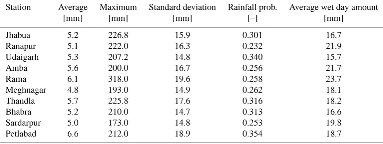
Table 1. Statistical properties of daily rainfall data for various stations of Anas catchment during the monsoon season.
Station Average Maximum Standard deviation Rainfall prob. Average wet day amount [mm] [mm] [mm] [–] [mm]
Jhabua 5.2 226.8 15.9 0.301 16.7 Ranapur 5.1 222.0 16.3 0.232 21.9 Udaigarh 5.3 207.2 14.8 0.340 15.7 Amba 5.6 200.0 16.7 0.256 21.7 Rama 6.1 318.0 19.6 0.258 23.7 Meghnagar 4.8 193.0 14.9 0.262 18.1 Thandla 5.7 225.8 17.6 0.316 18.2 Bhabra 5.2 210.0 14.7 0.313 16.6 Sardarpur 5.0 173.0 14.8 0.253 19.8 Petlabad 6.6 212.0 18.9 0.354 18.7
much weaker influence of the Coriolis force in the tropical latitudes it is not clear whether this approach, that has been successfully applied for precipitation downscaling in central and southern Europe (Stehlik and B´ardossy, 2002; B´ardossy and Filiz, 2005), is applicable at all. In a second compan-ion paper (Zehe et al., 2006) we will present an analysis of monsoon rainfall observed in the Anas catchment, with spe-cial emphasis of the spatial and temporal (auto-) correlation structure, as well as rainfall simulations for the Anas catch-ment with a multivariate stochastic rainfall model that uses time series of CPs as large scale meteorological forcing.
The present paper is organised as follows. After present-ing the study area and data base in Sect. 2, we will explain the CP classification methodology and the statistical meth-ods we employ for testing whether circulation patterns are suitable predictors for catchment scale rainfall in the Anas catchment 3. After presenting the results in Sect. 4 we close with discussion and conclusions in Sect. 5.
2 Research area and data records
The Anas catchment is a head watershed of the Mahi river basin which falls under a semiarid climatic zone in North Western India. The catchment covers a geographical area of 1750 km2with a mean altitude ranging from 280 m to 560 m (Fig. 1, compare Fig. 5 for the location of the Anas catch-ment in India). Daily rainfall data records for 10 stations were provided from the State Water Data Centre (SWDC) at Bhopal. Since 80–90% of the rainfall occurs during the monsoon season (June to October) rainfall data were only available for this period of the year. In a first step this data had to be digitized to allow a statistical analysis.
The average daily rainfall amount, the observed maxi-mum, the standard deviation, and the average rainfall prob-ability as well as the average rainfall amount at a wet day are listed in Table 1. Daily rainfall probabilities during the monsoon period range from 0.25 to 0.35, the average rainfall
amounts at a wet day are with 16 to 25 mm quite high. The total rainfall in the monsoon season which provides 90% of the total annual rainfall ranges from 350 mm to 1300 mm for dry to wet years, respectively. Although 1300 mm per year appears to be quite high the climate is nevertheless semi-arid due to the high annual potential evaporation and the concentration of all the available precipitation on a period of 4 months. The rainfall station at Jhabua has the longest records ranging from 1957–1995. Records at Thandla range from 1964–1995 and the data records at the remaining sta-tions range from 1985–1994. A more thorough analysis of the observed precipitation at the ten stations with respect to the average spatial correlation and the average autocorrela-tion is given in the companion paper (Zehe et al., 2006).
3 Methodology
3.1 Classification of circulations patterns 3.1.1 Basic idea of the downscaling approach
Stehlik and B´ardossy (2002) developed a methodology for generating spatio-temporal variable precipitation data using large scale daily pressure fields (simulated or observed) as well as local scale precipitation. The method consists of two main steps:
– An optimisation of fuzzy rules to classify pressure fields
into circulation patterns (CPs), to explain the basin scale space-time variability of observed rainfall.
– A multivariate and stochastic generation of rainfall at
a function of the actual CP as well as of the day in the year. The annual cycles of the spatial covariance func-tion and of the one day lag autocorrelafunc-tion are described by means of a Fourier series.
Why do we select circulation patterns as predictor and not di-rectly use the pressure data and additional predictors for pre-dicting monsoon precipitation e.g. by employing expanded downscaling suggested by B¨urger (2002)? As will become clear in the next section the CPs are able to discriminate the spatial locations where high or low pressure values are im-portant for precipitation for the target area from those loca-tions with no influence. This is a) an important insight and leads b) to an enormous gain in computation time, because a pressure pattern time series is a scalar predictor, that embeds the information on the spatial pressure pattern with it. As the focus of the present study is on the question whether pres-sure patterns are useful predictors for explaining space-time variability of precipitation in the Anas catchment, we omit further information on the multivariate rainfall model. In-terested readers will find detailed information in Stehlik and B´ardossy (2002) as well as in the companion paper (Zehe et al., 2006).
3.1.2 Definition of fuzzy rules and objective functions Input into CP classification is in principle daily geo-potential data from a selected level e.g. 700 or the 500 HPa from the NCEP data set. In the first step the pressure data are trans-formed to standardised anomalies by subtracting the long term monthly average from the actual value at each node and dividing the resulting difference by the long term monthly standard deviation. The basic idea of assessing a CP or pres-sure pattern classification scheme is to identify a set of dis-tinct locations in a spatial window where the configuration of pressure anomalies is on average associated with drier or wetter than average atmospheric conditions. Based on tri-angular fuzzy membership functions the daily anomalies at each location (x, y) are classified into the categories 1) high, 2) medium high, 3) medium low, 4) low or 5) indifferent for the circulation pattern. The membership functions for the five categories are v=1, low: (−2.0, −1,−0.2)T; v=2, medium low: (−1.4,−0.6,0)T; v=3, medium high: (0, 0.6, 1.4)T; v=4, very high: (0.2, 1, 2.0)T; and v=5 indifferent, constant as 1. Please note that the category “indifferent” is essential, as it allows separation of important locations from those which are not important.
Thus a circulation pattern, CPk, is fully characterised by an index vectorv(k)={v(1)(k)...v(n)(k)}that defines the lo-cations of heights and depressions in the pressure window according to four categories. As a rule of thumb the anoma-lies at 10–12 locations in the windows is important, the rest is indifferent and is not stored, and a set of 10–12 circula-tion patterns is a good choice (Stehlik and B´ardossy, 2002). A pressure field for a given day is classified into a circula-tion pattern by calculating the degree of fulfilment (DOF) for
each rule based on the membership values,µ, of the actual pressure anomaly value at each node in the window and se-lecting the CP with the highest DOF (B´ardossy et. al., 2002). To find out which locations are important as well as to op-timise the CP classification scheme the selection of suitable objective functions is of highest importance. Following the approach of Stehlik and B´ardossy (2002) we defined:
O1= S X
i=1 v u u t 1 Nd Nd X
t=1
(p(CP(t ))i− ¯p)2 (1)
where S is number of stations with precipitation observa-tions,Ndis the number of days in the time series,p(CP(t ))i is the CP-conditional probability of a wet day at stationi,p¯i is the total average probability at stationi. High values ofO1 indicate that the conditional rainfall probabilities of the CPs differs strongly from the average values i.e. represent drier or wetter than average meteorological conditions for the area. Stehlik and B´ardossy (2002) propose a second objectiveO2 based on the conditional precipitation amountsz(CP):
O2= S X
i=1 1
Nd Nd X
t=1 log z
p(CP(t ))i
¯ zp,i (2)
wherez¯i is the overall average daily precipitation amount at station i. High values of O2 indicate that the conditional rainfall amount of a CP differ clearly from the average value. Within the optimization we used the sum ofO1andO2as one possible objective functionO. However, the log transforma-tion in Eq. (2) puts a stronger weight on the small and average daily precipitation amounts as the logarithm is a very slowly increasing function. Alternatively, to assign higher weights to high and extreme daily precipitation values within the op-timisation we defined an objective functionO20 based on the conditional precipitation amounts z(CP):
O20= S X
i=1 1
Nd Nd X
t=1
z(CP(t )) i zi b (3)
The total objective function,O0, was again the sum ofO1 andO20, with an exponentb=1 or 1.5.
E. Zehe et al.: Assessment of objective circulation patterns 801
Fig. 2. Wetness index of the 500 HPa CPs plotted for 6 rain gauges (defined according to Eqs. 4 and 5). Values larger than 1 indicate that the
CP combines higher than average daily rainfall probabilities with higher than average conditional rainfall amounts. The figure header show the values of the objective functionO2(Eq. 1), the higher the values the better does the classification scheme separate between dry and wet
CPs.
Fig. 3. Wetness index of the 500 HPa CPs plotted for 6 rain gauges (defined according to Eqs. 4 and 5). Values larger than 1 indicate that the
CP combines higher than average daily rainfall probabilities with higher than average conditional rainfall amounts. The figure headers show the values of the objective functionO2(Eq. 1).
3.2 Quality assessment of the classification scheme
Within the present study the following classification schemes were tested: a set of 10 or 12 CPs, classified either from the 500 HPa pressure level or the 700 HPa pressure level on a 2.5◦by 2.5◦grid. As spatial window we selected 5◦N 40◦E and 35◦N 95◦E which covers the Indian subcontinent as well
as large parts of the Arabian Sea and the Gulf of Bengal. Furthermore, we compared the objective functionsOandO0
for the exponents ofb=1 and 1.5 respectively.
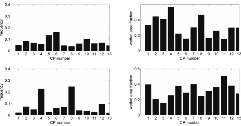
[image:5.595.98.499.353.560.2]Fig. 4. Average CP frequency and average wetted area fraction, which denotes the average fraction of rain gauges where rainfall is observed,
when weather is governed by a CP. The upper two panels denote the 500 HPa CPs, the lower two the 700 HPa CPs.
– The normalized conditional rainfall probability,np, de-fined as the conditional probability of precipitation at station i given the condition that the pressure at a day is classified into a given CP divided by the average pre-cipitation probability,pi, at this station. A strong devi-ation ofnpfrom 1 indicates that the conditional rainfall probability of the CP is much higher or lower than the average.
np=
pi(CP)
pi
(4)
– The normalized conditional rainfall amount,nz, defined as the conditional average precipitation amount on a wet day for a given CPzi(CP) at stationi divided by the average precipitation amount, zi, of a wet day at that station. A strong deviation ofnz from 1 indicates that the conditional rainfall amount of the CP is much higher or lower than the average:
nz=
zi(CP)
zi
(5)
The product ofnzandnp, named the wetness index, is a joint measure of whether the CP combines a higher/lower than average conditional rainfall probability with a higher/lower than average conditional rainfall amount.
Furthermore, to shed light on the significance of the CP conditional rainfall probabilities we selected the three wettest and the three driest CPs of the classification schemes with largest/smallest values for nz andnp obtained for the 700 and the 500 HPa level respectively. Next we took 1000 boot-straps from the precipitation time series at each of the ten
locations and computed the CP conditional rainfall probabil-ities for each bootstrap by frequency analysis for each of the selected CPs. The values were ranked in ascending order and we computed the fraction of bootstraps that were below the CP conditional probabilities. For the wet CPs the fraction of the bootstraps that are below has to be close to one to indi-cate that the significance of high precipitation probabilities is high. For the dry CPs it has to be the other way around: the number bootstraps that exceed the CP conditional rainfall probability has to be close to one to indicate that the classifi-cation is highly significant with respect to dry CPs.
Finally we computed the monthly frequencies of occur-rence for each CP within the classification scheme and cor-related them to the monthly rainfall totals as well as the monthly number of days observed at the 10 rain gauges. For optimising the CP classification scheme we selected the pe-riod from January 1985 to December 1994.
4 Results
4.1 CP classification schemes for 700 and 500 HPa The first criteria for selecting a CP classification scheme are high values of the objective function. For both pressure lev-els a set of 12 CP in combination with the objective function
E. Zehe et al.: Assessment of objective circulation patterns 803
Figure 5. Spatial distribution of 500hPa geo-potential height anomalies for the wet CP 4 (upper panel) and the dry CP 9 (lower panel), high values are shown in solid dark red lines while low pressure anomalies in solid blue lines.
17
Fig. 5. Spatial distribution of 500 hPa geo-potential height
anoma-lies for the wet CP 4 (upper panel) and the dry CP 9 (lower panel), high values are shown in solid dark red lines while low pressure anomalies in solid blue lines.
note that values around one indicate that the CP is associated with average rainfall conditions during the monsoon season. Wetness indices higher/lower than 1 indicate that the CP rep-resents drier or wetter than average weather conditions. The figure headers list, additionally to the station names, the val-ues of the objective functionO1 (defined in Eq. 1). The higher the values the better the does the classification scheme separate between dry and wet weather situations.
The classification scheme for the 500 HPa level separates dry from wet circulation patterns much more clearly than the classification scheme for the 700 HPa level pressure level. CP2, CP4 and CP8 from the 500 HPa level are associated in with atmospheric conditions that are more than twice as wet as the average. CP9, CP11 and CP6 result in much drier than average conditions in the Anas catchment. For the 700 HPa level CP11, CP12 and CP7 yield wet conditions, although their wetness index is smaller as in the case of the 500 HPa level. CP2, CP3 and CP6 represent on average dry meteoro-logical conditions.
Figure 4 presents the average CP frequency and average wetted area fraction, which denotes the average fraction of
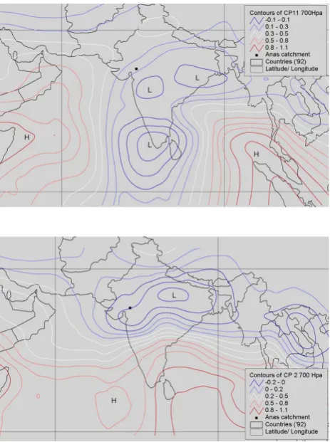
Figure 6. Spatial distribution of 700hPa geo-potential height anomalies for the wet CP 11 (upper panel) and the dry CP 2 (lower panel), high values are shown in solid dark red lines while low pressure anomalies in solid blue lines.
18
Fig. 6. Spatial distribution of 700 hPa geo-potential height
anoma-lies for the wet CP 11 (upper panel) and the dry CP 2 (lower panel), high values are shown in solid dark red lines while low pressure anomalies in solid blue lines.
rain gauges where rainfall is observed when weather is gov-erned by a CP. The upper two panels belong to the 500 HPa CPs, the lower two to the 700 HPa CPs. The wet CP2 for the 500 HPa level yields an average precipitation coverage of almost 60% of the rain gauges, the dry CP9 causes in a coverage of only 18%. In case of the 700 HPa the wet/dry CPs are also associated with a larger/smaller fraction of the catchment by precipitation, but the differences are less pro-nounced. Due to the more even occurrence frequencies of the CPs of the 500 HPa level the classification scheme has a higher entropy than the 700 HPa classification scheme. In the 700 HPa level CP4 and CP8, which are both associated with average rainfall conditions, dominate almost 50% of the time.
rang-Table 2. Frequency of bootstraps who’s CP conditional rainfall probability was below the ones calculated for the original time series for the
wet circulation patterns CP11 CP7 and CP12, as well as for the dry ones CP8, CP2 and CP3 in the 500 HPa level. In case of the wet CP the fraction is an estimator for the significance of the CP conditional rainfall probability, for the dry CPs one minus the fraction estimates the significance level.
CP 1 2 3 4 5 6 7 8 9 10
CP 4 1.000 1.000 1.000 1.000 1.000 1.000 1.000 1.000 1.000 1.000 CP 8 1.000 0.999 0.999 0.978 1.000 0.999 1.000 0.992 0.985 1.000 CP 2 0.998 1.000 1.000 1.000 1.000 1.000 1.000 1.000 0.999 0.998 CP11 0.000 0.009 0.000 0.001 0.000 0.063 0.000 0.002 0.000 0.002 CP 6 0.000 0.000 0.000 0.000 0.000 0.000 0.000 0.000 0.000 0.000 CP 9 0.001 0.016 0.001 0.042 0.011 0.000 0.000 0.024 0.002 0.000
1 = Jhabua, 2 = Ranapur, 3 = Udaigarh, 4 = Amba, 5 = Rama, 6 = Meghnagar, 7 = Thandla, 8 = Bhabra, 9 = Sardapur, 10 = Petlabad
Table 3. Frequency of bootstraps who’s CP conditional rainfall probability was below the ones calculated for the original time series for the
wet circulation patterns CP11 CP7 and CP12, as well as for the dry ones CP6, CP2 and CP3 in the 700 HPa level. In case of the wet CP the fraction is an estimator for the significance of the CP conditional rainfall probability, for the dry CPs one minus the fraction estimates the significance level.
CP 1 2 3 4 5 6 7 8 9 10
CP11 1.000 0.948 0.987 0.944 1.000 0.999 1.000 0.996 1.000 1.000 CP 7 0.998 0.993 0.999 0.993 0.989 0.996 0.983 0.990 1.000 0.985 CP12 0.993 0.997 1.000 0.914 0.980 0.993 0.994 0.998 1.000 0.892 CP 6 0.051 0.015 0.004 0.054 0.074 0.041 0.038 0.008 0.052 0.054 CP 2 0.005 0.048 0.000 0.060 0.070 0.054 0.085 0.011 0.001 0.095 CP 3 0.002 0.034 0.000 0.001 0.005 0.055 0.028 0.002 0.068 0.001
1 = Jhabua, 2 = Ranapur, 3 = Udaigarh, 4 = Amba, 5 = Rama, 6 = Meghnagar, 7 = Thandla, 8 = Bhabra, 9 = Sardapur, 10 = Petlabad
ing from the Indian Ocean to Mongolia which causes dry and hot weather conditions. For comparison Fig. 6 shows the average locations of the highs and depressions associated with the wettest CP11 and the dry CP2 in the 700 HPa level. CP11 in the 700 HPa appears with a pronounced depression with kernel in South West India similar to the wet CP4 in the 500 HPa level. CP2 is quite different: a strong depression over north-eastern India combined with an anticyclone lo-cated South-West from the Malabar Coast is expected to lead moist air from the Arabian Sea to central India. However, the Anas catchment should receive dry air from the North-Eastern part of India, that has to pass the mid-mountain bar-rier at the East of the catchment. Hence, it is associated with drier weather conditions.
4.2 Significance CP conditional rainfall probabilities Table 2 lists the fraction of the bootstraps whose CP condi-tional rainfall probability was below the values calculated for the original time series for the wet circulation patterns CP11 CP7 and CP12, as well as for the dry ones CP8, CP2 and CP3 in the 500 HPa level. In the case of a wet CP this fraction is an estimator for the significance of the CP conditional rain-fall probability. For dry CPs the significance level is obtained
by subtracting the fraction from one. The significance of the conditional rainfall probabilities for the wet as well as for the dry CPs is for all rain gauges larger than 95%. As can be seen in Table 3 the significance of the conditional rainfall proba-bilities for the wet CPs CP11, CP12 and CP 7 in the 700 HPa is similarly high as for the 500 HPa scheme. The significance of the dry CPs CP2, CP3, and CP6 is a little weaker as for the 500 HPa scheme
E. Zehe et al.: Assessment of objective circulation patterns 805
Table 4. Correlation between the monthly frequency of the wet and dry CPs in the 500 HPa level with the monthly number of rainy days at
the different rain gauges during the Monsoon season.
CP 1 2 3 4 5 6 7 8 9 10
CP 2 0.329 0.257 0.330 0.402 0.250 0.349 0.238 0.337 0.374 0.263 CP 4 0.349 0.400 0.374 0.359 0.415 0.358 0.401 0.313 0.313 0.456 CP 8 0.156 0.168 0.162 0.165 0.214 0.156 0.184 0.147 0.169 0.200 CP 6 −0.223 −0.313 −0.361 −0.382 −0.301 −0.405 −0.399 −0.319 −0.332 −0.399 CP 9 −0.355 −0.332 −0.318 −0.270 −0.347 −0.376 −0.372 −0.310 −0.370 −0.372 CP11 −0.286 −0.246 −0.232 −0.258 −0.251 −0.186 −0.219 −0.132 −0.228 −0.201
1 = Jhabua, 2 = Ranapur, 3 = Udaigarh, 4 = Amba, 5 = Rama, 6 = Meghnagar, 7 = Thandla, 8 = Bhabra, 9 = Sardapur, 10 = Petlabad
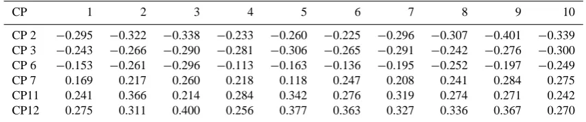
Table 5. Correlation between the monthly frequency of the wet and dry CPs in the 700 HPa level with the monthly number of rainy days at
the different rain gauges during the Monsoon season.
CP 1 2 3 4 5 6 7 8 9 10
CP 2 −0.295 −0.322 −0.338 −0.233 −0.260 −0.225 −0.296 −0.307 −0.401 −0.339 CP 3 −0.243 −0.266 −0.290 −0.281 −0.306 −0.265 −0.291 −0.242 −0.276 −0.300 CP 6 −0.153 −0.261 −0.296 −0.113 −0.163 −0.136 −0.195 −0.252 −0.197 −0.249 CP 7 0.169 0.217 0.260 0.218 0.118 0.247 0.208 0.241 0.284 0.275 CP11 0.241 0.366 0.214 0.284 0.342 0.276 0.319 0.274 0.271 0.242 CP12 0.275 0.311 0.400 0.256 0.377 0.363 0.327 0.336 0.367 0.270
1 = Jhabua, 2 = Ranapur, 3 = Udaigarh, 4 = Amba, 5 = Rama, 6 = Meghnagar, 7 = Thandla, 8 = Bhabra, 9 = Sardapur, 10 = Petlabad
5 Discussion and conclusions
The presented results give clear evidence that objective cir-culation classified patterns especially from the 500 HPa level are suitable to explain the spatio-temporal variability of mon-soon rainfall within the Anas catchment. The CP condi-tional rainfall probabilities of the wettest and the driest CPs are highly significant. Furthermore, 30% of the variation of the monthly number of rainy days at all stations may be ex-plained by the occurrence frequency of the three wettest CPs of the 500 HPa level. Shukla and Mooley (1987) found a similar strong relation between the EL Nino Southern Oscil-lation (ENSO) and the temporal monsoon variability over the India.
Near to the Equator one would of course expect the CPs from 700 HPa level, which are in average located at a height of 3000 m, to have a stronger influence. However, as the Anas catchment is located approximately 23◦north, the
Cori-olis parameter is of order 0.4. Although this is only half as large as in the mid-latitudes, the influence of the Coriolis force seems still large enough that the CPs from the 500 HPa level are the better predictors.
The overall objective of this study was to give evidence that objectively classified pressure patterns are suitable predictors for monsoon rainfall in North West India, despite the low influence of the Coriolis force. We may state that this goal has been successfully achieved. However, the identification of a suitable predictor is only the first essential
step towards modelling monsoon precipitation by means of empirical downscaling. The next essential step, which is addressed in the companion paper (Zehe et al., 2006), is to establish a suitable predictive relationship between the predictors and the rainfall in the Anas catchment. This is achieved by means of a multivariate stochastic model originally proposed by Stehlik and B´ardossy (2002) which uses CP time series as large scale meteorological forcing. Either pressure fields from reanalysis data or from climate model runs maybe be classified into such a CP time series. The proposed approach may be used for generating historical rainfall time series for e.g. for water resources planning as well as for questions of climate impact assessment. Interested readers shall therefore refer to Zehe et al. (2006).
Edited by: M. Sivapalan
References
B´ardossy, A. and Filiz, F.: Identification of flood producing atmo-spheric circulation patterns, J. Hydrol., 313, 48–57, 2005. B´ardossy, A., Stehlik, J., and Caspary, H.-J.: Automated objective
classification of daily circulation patterns for rainfall and temper-ature downscaling based on optimised fuzzy rules, Clim. Res., 23, 11–22, 2002.
[image:9.595.83.511.253.342.2]B´ardossy, A., Duckstein, L., and Bog´ardi, I.: Fuzzy rule based clas-sification of atmospheric circulation patterns, Int. J. Climatol., 15, 1087–1097, 1995.
Bamzai, A. S. and Shukla, J.: Relation between Eurasian snow cover, snow depth and the Indian summer monsoon: An obser-vational study, J. Clim., 12, 3117–3132, 1999.
Bogardy, I., Matyasovszky, I., Bardossy, A., and Duckstein, L.: A hydro-climatological model of areal droughts, J. Hydrol., 153, 245–264, 1994.
Bergstrom, S. Carlson, B., Gardekin, M., Lindstrom, G., Peterson, A., and Rummukainen, M.: Climate change impacts on Hydrol-ogy in Sweden – assessment by global circulation models, dy-namical downscaling and hydrological modelling, Clim. Res., 16, 101–112, 2001.
B¨urger, G.: Selected precipitation scenarios across Europe, J. Hy-drol., 262, 99–110, 2002.
Clark, C. O, Cole, J. E., and Webster, P. J.: Indian ocean SST and In-dian summer rainfall: Predictive relationships and their decadal variability, J. Clim., 13, 2503–2519, 1999.
Clarke, M. P., Hay, L. E., McCabe, G. J., Leavesley, G. H., Ser-reze, M. C., Wilby, R. L.: The use of weather and climate infor-mation in management of water resources in the western United States, Proceedings of the Special Conference on Climate Vari-ability and Water Resources, NOAA, Boulder, USA, 2001. Conway, D. and Jones, P. D.: The use of weather types and airflow
indices for GCM downscaling, J. Hydrol., 213, 348–361, 1998. Dickson, R. R.: Eurasion snow cover versus Indian monsoon
rain-fall. An extension of the Hahn – Shukla results, J. Clim. Appl. Meteor., 23, 171–173, 1984.
Frei, C., Schar, C., Luthi, D., and Davies, H. C.: Heavy precipitation processes in a warmer climate, Geophys. Res. Lett., 25, 1431– 1434, 1998.
Giorgi, F. , Mearns, L. O., Shields, C., and McDaniel, L.: Regional nested model simulations of present and 2x CO2climate over the
central plains of the US, Clim. Change, 40, 457–493, 1999. Gowarikar, V., Thapliyal, V., Kulshrestha, S. M., Mandal, G. S., Sen
Roy, N., Sikka, D. R.: A power regression model for long range forecast of south-west monsoon rainfall over India, Mausam, 42, 125–130, 1991.
Harzallah, A. and Sadourny, R.: Observed lead lag relationships between Indian summer monsoon and some meteorological vari-ables, Clim. Dyn., 13, 635–648, 1999.
Hess, P. and Brezowsky, H.: Katalog der Großwetterlagen Europas. 2. neu bearb. u. erg. Aufl., Berichte des Deutschen Wetterdien-stes 113; Selbstverlag des DWD, Offenbach a.M., Deutschland, 1969.
Jacob, D., van den Hurk, J. J. M., Andrae, U., Elgered, G., Fortelius, C. Graham, L. P., Jackson, S, D., Karstens, U., K¨opken, Chr. Lindau, R. Podzun, R., Rockel, B. Rubel, F. Sass, B. H., Smith, R. N. B., and Yang, X.: A comprehensive model inter-comparison study investigating the water budget during the BALTEX-PIDCAP period, Meteorol. Atmos. Phys., 77, 19–43, 2001.
Kunstmann, H. and Jung, G.: Investigation of feedback mecha-nisms between soil moisture, landuse and precipitation in West Africa, Water Resources System, Water Availiability and Global Change, IAHS Publications 280, 159–159, 2003.
Maheras, P.: The synoptic weather types and objective delimitation of the winter period in Greece, Weather, 43, 2, 40–45, 1988. Maheras, P.: Delimitation of the Summer-dry period in Greece
ac-cording to the frequency of weather-types, Theor. Appl. Clima-tol., 39, 171–176, 1989.
MoE India: India’s National Communication of the UNFCCC, Min-istry of Environment and Forests, Government of India, Delhi, 2004.
Press, W. H., Teukolsky, S. A., Vetterling, W. T., and Flannery, B. P.: Numerical Recipes in FORTRAN: The Art of Scientific Com-puting, Cambridge University Press, 1992.
¨
Ozelkan, E., Galambosi, L., Duckstein, L., and B´ardossy, A.: A multi-objective fuzzy classification of large scale circulation pat-terns for precipitation modeling, Appl. Math. Comp., 91, 127– 142, 1998.
Shukla, J. and Mooley, D. A.: Empirical prediction pf the sum-mer monsoon rainfall over India, Mon. Wea. Rev., 115, 695–703, 1987.
Siddiq, E. A.: Rainfall prediction for rice growing areas, in: Rice in a variable climate, edited by: Abrol, Y. P. and Gadgil, S., APC Publication Delhi, pp. 107–123, 1999.
Stehlik, J. and Bardossy, A.: Multivariate stochastic downscaling model for generating daily Rainfall series based on atmospheric circulation, J. Hydrol., 256, 120–141, 2002.
Webster, P. J. and Hoyos, C.: Prediction of monsoon rainfall and river discharge on 15–30 day time scales, Bull. Amer. Meteor. Soc., 85, 1745–1767, 2004.
W´ojcik, R. and Buishand, T. A.: Simulation of 6-hourly rainfall and temperature by two resampling schemes, J. Hydrol. 273, 1– 4, 69–80, 2003.
Wilby, R. L. and Wigley, T. M. L.: Precipitation predictors for downscaling – observed and general circulation model relation-ships, Int. J. Climatol., 20, 641–661, 2000.
Wilby, R. L,. Hay, L. E., and Leavesly, G. H.: A comparsion of downscaled and raw GCM output: implications for climate change scenarios in the San Juan River basin, Colorado, J. Hy-drol., 225, 67–91, 1999.
Wilby, R. L. and Wigley, T. M. L.: Downscaling general circulation model output: a review of methods and limitations, Prog. Phys. Geogr., 21, 530–548, 1997.