Tabu Search Based Interactive Fuzzy Stochastic Multi Level 0 1 Programming

Tabu Search-Based Interactive Fuzzy Stochastic

Multi-Level 0-1 Programming

Masatoshi Sakawa

∗

,

Takeshi Matsui

Faculty of Engineering, Hiroshima University, Higashi-Hiroshima, 739-8527, Hiroshima, Japan

∗_{Corresponding Author: sakawa@hiroshima-u.ac.jp}

Copyright c2013 Horizon Research Publishing All rights reserved.

Abstract

This paper considers interactive fuzzy programming for multi-level 0-1 programming problems involving random variable coefficients both in objective functions and constraints. Following the concept of fractile criterion optimization together with chance constrained programming, the formulated stochastic multi-level 0-1 programming problems are transformed into deterministic ones. Taking into account vagueness of judgments of the decision makers, interactive fuzzy programming is presented. In the proposed interactive method, after determining the fuzzy goals of the decision makers at all levels, a satisfactory solution is derived efficiently by updating satisfactory levels of the decision makers with considerations of overall satisfactory balance among all levels. For solving the transformed deterministic problems efficiently, tabu search for general 0-1 programming problems is introduced. An illustrative numerical example for a three-level 0-1 programming problem is provided to clarify the proposed method.

Keywords

Multi-level 0-1 programming, Random variables, Interactive fuzzy programming, Fractile criterion optimization, Tabu search

1

Introduction

In the real world, we often encounter situations where there are two or more decision makers (DMs) in an or-ganization with a hierarchical structure, and they make decisions in turn or at the same time so as to optimize their objective functions. Such situations are formulated as multi-level programming problems, and the Stackel-berg solution has been usually employed as a solution concept [1].

When the Stackelberg solution is employed, it is as-sumed that there is no communication between the two DMs, or they do not make any binding agreement even if there exists such communication. However, the above assumption is not always reasonable when we model de-cision making problems in a decentralized firm as a two-level programming problem in which top management is a leader and an operation division of the firm is a

follower because it is supposed that there exists cooper-ative relationship between them.

For two-level linear programming problems or multi-level ones such that decisions of decision makers in all levels are sequential and all of the decision makers es-sentially cooperate with each other, Lai [2] and Shih et al. [3] proposed fuzzy interactive approaches. In their methods, the decision makers identify membership func-tions of the fuzzy goals for their objective funcfunc-tions, and in particular, the decision maker at the upper level also specifies those of the fuzzy goals for the decision vari-ables. The decision maker at the lower level solves a fuzzy programming problem with a constraint with re-spect to a satisfactory degree of the decision maker at the upper level.

Unfortunately, however, there is a possibility that the methods of Lai [2] and Shih et al. [3] lead a final solution to an undesirable one because of inconsistency between the fuzzy goals of the objective function and those of the decision variables. In order to overcome the problem in their methods, by eliminating the fuzzy goals for the decision variables, Sakawa et al. have proposed interac-tive fuzzy programming for two-level or multi-level linear programming problems to obtain a satisfactory solution for decision makers [4, 5]. Extensions to two-level linear fractional programming problems [5] and decentralized two-level linear programming problems [6–8] have also been considered. The subsequent works on two-level or multi-level programming have been appearing [9–12]. A recent survey paper of Sakawa and Nishizaki [13] is de-voted to reviewing and classifying the numerous major papers in the area of so-called cooperative multi-level programming.

concepts have been studied by many researchers [17,18]. Fuzzy multiobjective linear programming, first proposed by Zimmermann [17], have been also developed by nu-merous researchers, and an increasing number of suc-cessful applications has been appearing [18,19,22,23]. In particular, after reformulating stochastic multiobjective linear programming problems using several models for chance constrained programming, Sakawa et al. [24–26] presented an interactive fuzzy satisficing method to de-rive a satisficing solution for the DM as a generalization of their previous results [18, 22, 23, 27–30].

Furthermore, in real world decision making situations, it is often found that decision variables in a multiob-jective stochastic programming problem the formulated programming problems are not continuous but rather discrete. To deal with practical sizes of the stochas-tic multi-level 0-1 programming problems formulated for decision making problems in the real world, an efficient tabu search method for general 0-1 programming prob-lems is introduced.

Under these circumstances, in this paper, through a simultaneous consideration of both random variables and integer decision variables involved in the real world hierarchical decision making problems, we first formu-late multi-level 0-1 programming problems with random variable coefficients in both objective functions and con-straints. The main contribution of this paper is to pro-vide a novel decision making methodology including a new model, solution concept and solution algorithm to deal with more realistic problems in the real world, by simultaneously considering various concepts such as hi-erarchy structure, fuzziness, randomness, 0-1 decision variables and interactive fuzzy programming, while most of previous papers dealt with either of the concepts or a part of them.

By employing chance constrained programming [31], stochastic constraints are transformed into determinis-tic ones. Adopting the fractile criterion optimization model [32,33], the minimization of each stochastic objec-tive function is replaced with the optimization of the tar-get variables under the condition that the attained prob-abilities are greater than or equal to certain permissible levels. Under some appropriate assumptions for distri-bution functions, the formulated stochastic multi-level 0-1 programming problems are transformed into deter-ministic ones. In our interactive method, after determin-ing the fuzzy goals of the DMs at all levels, a satisfactory solution is derived efficiently by updating the satisfac-tory degrees of the DMs at the upper level with consid-erations of overall satisfactory balance among all levels. For solving the transformed deterministic problems effi-ciently, we also propose a novel tabu search method by extending tabu search based on strategic oscillation for multidimensional 0-1 knapsack problems [34] into gen-eral 0-1 programming problems.

2

Problem formulation with

frac-tile models

Consider stochastic multi-level 0-1 programming problems where each of the DMs at all levels takes over-all satisfactory balance among over-all levels into

considera-tion and tries to optimize each objective funcconsidera-tion. Such a stochastic multi-level 0-1 programming problem can be formulated as

minimize

DM1 (Level 1) z1(x) =c11(ω)x1+· · ·+c1K(ω)xK ..

. ...

minimize

DMK(LevelK) zK(x) =cK1(ω)x1+· · ·+cKK(ω)xK subject to A1x1+· · ·+AKxK ≤b(ω)

x1∈ {0,1}n1, . . . ,xK ∈ {0,1}nK

                

(1) wherexl, l= 1, . . . , K, is annl-dimensional 0-1 decision

variable column vector,Al, l= 1, . . . , K arem×nl

co-efficient matrices, andclj(ω),l= 1, . . . , K,j= 1, . . . , K

are nj-dimensional Gaussian random variable row

vec-tors with mean vecvec-tors ¯clj, and covariance matrices

Vlpq =

v_hl_phq= Cov[clhp(ω), clhq(ω)]

, p= 1, . . . , K,

q = 1, . . . , K, and they are independent of each other, andb(ω) is a random variable vector whose joint distri-bution function isF(·).

Since (1) contains random variable coefficients, solu-tion methods for ordinary mathematical programming problems cannot be applied directly. Consequently, we first deal with the constraints in (1) as chance con-straints [21] which mean that the concon-straints need to be satisfied with a certain probability (satisficing level) and over. Namely, replacing constraints in (1) by chance constraints with a satisficing levelβ, the problem can be transformed as:

minimize

DM1 (Level 1) z1(x) =c11(ω)x1+· · ·+c1K(ω)xK ..

. ...

minimize

DMK(LevelK) zK(x) =cK1(ω)x1+· · ·+cKK(ω)xK subject to Pr{ai1x1+· · ·+aiKxK≤bi(ω)}

≥βi, i= 1, . . . , m

x1∈ {0,1}n1, . . . ,xK∈ {0,1}nK

                    

(2) where aij is the ith row vector ofAl, l= 1, . . . , K, and

bi(ω) is theith element of b(ω).

The first constraint in (2) is rewritten as: Pr{ai1x1+· · ·+aiKxK≤bi(ω)} ≥βi

⇔ 1−Pr{ai1x1+· · ·+aiKxK ≥bi(ω)} ≥βi

⇔ 1−Fi(ai1x1+· · ·+aiKxK)≥βi

⇔ Fi(ai1x1+· · ·+aiKxK)≤1−βi

⇔ ai1x1+· · ·+aiKxK ≤Fi∗(1−βi)

where F_i∗ is a pseudo-inverse function of Fi.

Letting ˆbi=Fi∗(1−βi), problem (2) can be rewritten

as:

minimize DM1 (Level 1)

z1(x) =c11(ω)x1+· · ·+c1K(ω)xK

..

. ...

minimize DMK(LevelK)

zK(x) =cK1(ω)x1+· · ·+cKK(ω)xK

subject to A1x1+· · ·+AKxK ≤ˆb

x1∈ {0,1}n1, . . . ,xK ∈ {0,1}nK

                

(3) whereˆb= (ˆb1,ˆb2, . . . ,ˆbm)T.

Charnes and Cooper [31] also considered three types of decision rules for optimizing objective functions with random variables: (i) the minimum or maximum ex-pected value model, (ii) the minimum variance model, and (iii) the maximum probability model, which are re-ferred to as the expectation model, the variance model, and the probability model, respectively. Moreover, Kataoka [32] and Geoffrion [33] individually proposed the fractile model.

For instance, let the objective function represent a profit. If the DM wishes to simply maximize the ex-pected profit without caring about the fluctuation of the profit, the expectation model to optimize the expecta-tion of the objective funcexpecta-tion is appropriate. On the other hand, if the DM hopes to decrease the fluctuation of the profit as little as possible from the viewpoint of the stability of the profit, the variance model to mini-mize the variance of the objective function is useful. In contrast to these two types of optimizing approaches, as satisficing approaches, the probability model and the fractile model have been proposed.

When the DM wants to maximize the probability that the profit is greater than or equal to a certain permissible level, probability model is recommended. In contrast, when the DM wishes to optimize such a permissible level under a given threshold probability with respect to the achieved profit, the fractile model will be appropriate. In this paper, assuming that the DM is interested in the probability that each objective function attains a goal value rather than the expectation or variance of each membership function, we adopt the fractile criterion op-timization as a decision making model.

In the fractile criterion optimization model, the min-imization of each of objective function zl(x) in (3) is

substituted with the optimization of the target value that zl(x) is less than or equal to a certain permissible

level fl under the chance constraints. Through fractile

criteria optimization, problem (3) can be rewritten as:

minimize

DM1iLevel 1j f1

. .

. ... minimize

DMKiLevelKj fK

subject to Pr [c11(ω)x1+· · ·+c1K(ω)xK≤f1]

≥α1 .

. .

Pr [cK1(ω)x1+· · ·+cKK(ω)xK≤fK]

≥αK

A1x1+· · ·+AKxK≤ˆb x1∈ {0,1}n1, . . . ,xK ∈ {0,1}nK

                                   (4) Since all elements of clj(ω), l = 1, . . . , K,j = 1, . . . , K

are assumed to be Gaussian random variable with mean ¯

clj and covariance matrices Vlpq, p = 1, . . . , K, q =

1, . . . , K.

Then, (hl − (¯cl1x1 + · · · + ¯

clKxK))/

q

(xT

1, . . . ,xTK)Vl(xT1, . . . ,xTK)T is a random

variable following the standard Gaussian distribution with mean 0 and variance 1. Hence, we can rewrite the

objective functions in (4) as follows.

Pr{zl(x1, . . . ,xK, ω)≤fl}

= Pr{cl1(ω)x1+· · ·+clK(ω)xK≤fl}

= Pr (

cl1(ω)x1+· · ·+clK(ω)xK−(¯cl1x1+· · ·+ ¯clKxK) p

(xT

1, . . . ,xTK)Vl(xT1, . . . ,xTK)T

≤ _pfl−(¯cl1x1+· · ·+ ¯clKxK) (xT

1, . . . ,xTK)Vl(xT1, . . . ,xTK)T )

=φl

fl−(¯cl1x1+· · ·+ ¯clKxK) p

(xT

1, . . . ,xTK)Vl(x T

1, . . . ,xTK)T !

≥αl,

where φl(·) is the distribution function of the standard

Gaussian random variable. From the monotonicity of the distribution function, we can define the inverse func-tion φ−_l1(·) of φl(·). Then, the above inequalities are

expressed as:

fl−(¯cl1x1+· · ·+ ¯clKxK)

q

(xT

1, . . . ,xTK)Vl(xT1, . . . ,xTK)T

≥Kαl

⇔ fl≥(¯cl1x1+· · ·+ ¯clKxK)

+Kαl

q

(xT

1, . . . ,xTK)Vl(xT1, . . . ,xTK)T

Letting Kαl = φ

−1

l (αl), l = 1,· · · , K and noting that

the equality

fl= (¯cl1x1+· · ·+ ¯clKxK)

+Kαl

q

(xT

1, . . . ,xTK)Vl(xT1, . . . ,xTK)T

holds at the minimum of fl, problem (4) is equivalent

to the following deterministic multi-level programming problem:

minimize

DM1iLevel 1j Z

F

1(x1, . . . ,xK)

= (¯c11x1+· · ·+ ¯c1KxK) +Kα1

p (xT

1, . . . ,xTK)V1(xT1, . . . ,xTK)T

. .

. ...

minimize

DMKiLevelKj Z

F

K(x1, . . . ,xK)

= (¯cK1x1+· · ·+ ¯cKKxK) +KαK

p (xT

1, . . . ,xTK)VK(xT1, . . . ,xTK)T

subject to x∈X

                           (5) where X denotes the feasible region satisfying the con-straints of (4).

3

Interactive fuzzy programming

In the deterministic multi-level 0-1 programming problem (5), considering the vague nature of the DMs’ judgments for the target valuesZF

l (x), l= 1,2, . . . , Kit

seems natural to assume that the DMs have fuzzy goals such as “ZF

l (x) should be substantially greater than or

equal to some specific value.”

Through the introduction of a membership function

µl(·) for quantifying a fuzzy goal for thel th objective

function in (5), (5) can be rewritten as: maximize

DM1iLevel 1j µ1(Z

F

1(x1, . . . ,xK))

..

. ...

maximize

DMKiLevelKj µK(Z

F

K(x1, . . . ,xK))

subject to x∈X

whereµl(·) is assumed to be nondecreasing.

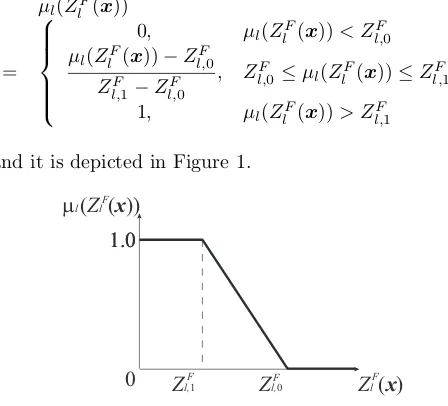
Although the membership function does not always need to be linear, for the sake of simplicity, we adopt a linear membership function. To be more specific, if the DM feels thatZ_lF(x) should be greater than or equal to at least Z_l,F₀ and Z_lF(x) ≥ Z_l,F₁(> Z_l,F₀) is satisfactory, the linear membership functionµl(ZlF(x)) is defined as:

µl(ZlF(x))

=

        

0, µl(ZlF(x))< Zl,F0

µl(ZlF(x))−Zl,F0

ZF l,1−Zl,F0

, ZF

l,0≤µl(ZlF(x))≤Zl,F1 1, µl(ZlF(x))> Z

F l,1

(7) and it is depicted in Figure 1.

1.0

0

1.0

µ

l

(

Z

l

(

x

))

Z

l

(

x

)

Z

l,1

Z

l,0

F F

[image:4.595.61.285.149.352.2]

F F

Figure 1. Linear membership function.

Zimmermann [17] suggested a method for assessing the parameter values of the linear membership function. In his method, the parameter values ZF

l,1, l = 1, . . . , K are determined as

ZF

1,1 =Z1F,max

=Z₁F(x1_1,max, . . . ,x1_K,max)

= max

(xT

1,...,xTK)T∈X

Z₁F(x1, . . . ,xK)

.. .

ZF

K,1 =ZK,Fmax

=Z_KF(xK1,max, . . . ,xKK,max)

= max

(xT

1,...,xTK)T∈X

Z_KF(x1, . . . ,xK)

and the parameter valuesX_l,F₀, l= 1, . . . , Kare specified as

Z1F,0=Z1F(x11,min, . . . ,x 1

K,min) ..

.

ZF

K,0=ZKF(x1K,min, . . . ,xKK,min)

where xl,min = (x1l,min, . . . ,xKl,min), l = 1, . . . , K is an optimal solution to the following problem

maximize ZF

l (x1, . . . ,xK)

=φl

 

fl−(¯cl1x1+· · ·+ ¯clKxK)

q

(xT

1, . . . ,xTK)Vl(xT1, . . . ,xTK)T

 

subject to x∈X

          

.

(8) Since (8) is a 0-1 programming problem, it can be solved by tabu search based on strategic oscillation [34]. Then, by setting the parameters as described above, the linear membership functions (7) is identified.

To derive an overall satisfactory solution to the mem-bership function maximization 6, we first find the max-imizing decision of the fuzzy decision proposed by Bell-man and Zadeh [35]. Namely, the following problem

is solved for obtaining a solution which maximizes the smaller degree of satisfaction between those of all DMs:

maximize

x∈X l=1min,...,K

µl(ZlF(x)) (9)

Solving problem (9), we can obtain a solution which maximizes the smaller satisfactory degree between those of all DMs.

Termination conditions of the interactive process (1) For allλ= 1, . . . , K−1, DMλ’s satisfactory degree

is larger than or equal to the minimal satisfactory level ˆδ∆λ specified by DMλ.

(2) For allλ= 1, . . . , K−1, the ratioδλ of satisfactory

degrees is in the closed interval the lower and the upper bounds of which are specified by DMλ. Condition (1) means DMλ’s required condition for solu-tions proposed by DM(λ+ 1). Condition (2) is provided in order to keep overal satisfactory balance among all the level.

Unless the conditions are satisfied simultaneously, DMλ, λ= 1, . . . , K, needs to update the minimal sat-isfactory level ˆδ∆λ. Suppose that the DMs from at the (q+ 1)th level to at the (K−1)th level, i.e., DM(q+ 1), DM(q+ 2), . . ., and DM(K−1), satisfy the proposed solution but DMq does not satisfy it. Then DMq, DM(q+ 1), . . ., and DM(K−1) need to update their minimal satisfactory levels ˆδ∆λ, λ=q, q+ 1, . . . , K−1. For any two levels adjacent to each other, giving a DM at an upper level serious consideration, a DM at a lower level should update the minimal satisfactory level.

Now we are ready to propose interactive fuzzy pro-gramming for deriving a satisfactory solution by up-dating the satisfactory degree of the DM at the upper level with considerations of overall satisfactory balance among all the levels.

Computational procedure of interactive fuzzy programming Step 1: Ask the decision maker at the upper level,

DM1, to subjectively determine a satisficing levels

αl ∈ (0,1), l = 1,2, . . . , K for objective functions

and βi ∈ (0,1), i= 1,2, . . . , m for constraints. Go

to Step 2.

Step 2: The following problems are solved to find the minimum values Z_l,F_min = Z_lF(xl,min) and Z_l,MF =

max

j=1,...,K{Z F

l (xj,min)} of objective functions ZlF(x)

under the chance constraints with satisficing levels

αl, l= 1,2, . . . , K andβi, i= 1,2, . . . , m.

minimize Z_lF(x1, . . . ,xK)

subject to x∈X

, l= 1, . . . , K

(10) If the set of feasible solutions to these problems is empty, the satisficing levels αl ∈ (0,1), l =

1,2, . . . , K and βi, i = 1,2, . . . , m must be

solved by tabu search based on strategic oscilla-tion. Then, identify the linear membership function

µl(ZlF(x)), l= 1,2, . . . , K of the fuzzy goal for the

corresponding objective function. Go to Step 3. Step 3: Solve the following corresponding maxmin

problem.

maximize

x∈X l=1min,...,K

µl(ZlF(x)) (11)

Go to step 4.

Step 4: Ask DM1 to subjectively set the minimal satis-factory level ˆδ1. Then, solve the following maxmin problem.

maximize

x∈X _l=2min_,...,K

µl(ZlF(x))

subject to µ1(p1(x))≥δˆ1

)

(12)

Setλ:= 2Cλ0 := 1. Go to step 5.

Step 5: Ask DMλ to set the membership function µ∆λ(∆λ(x)) for the ratio ∆λ = (µλ+1(ZλF+1(x)))/(µλ(ZλF(x))) of satisfactory

degrees and the minimal satisfactory level ˆδ∆λ. Solve the following maxmin problem.

maximize

x∈X _l=λmin_+1,...,K

µl(ZlF(x))

subject to µ1(Z1F(x))≥δˆ1

µ∆2(∆2(x))≥δˆ∆2

.. .

µ∆λ(∆λ(x))≥δˆ∆λ

              

(13)

Repeat this step untilλ=K−1.

Step 6: If the current solution satisfies the termination conditions, DMK−λ0 accepts it, andK−λ0 = 1, then the procedure stops and the current solution is determined to be a satisfactory solution. Otherwise, ask DMK−λ0 to update the minimal satisfactory level ˆδ∆K−λ0. IfK−λ

0_{= 1, ask DM1 to update the}

minimal satisfactory level ˆδ1. Go to step 7. Step 7: Solve the following problem, and return to step

5.

maximize v

subject to x∈X

0≤v≤1

µ1(Z1F(x))≥δˆ1

µ∆2(∆2(x))≥ˆδ∆2

.. .

µ∆K−1(∆K−1(x))≥δˆ∆K−1

Π_lK₌−_K1_−λ0₊₁∆ˆlµK−λ0₊₁(ZF

K−λ0₊₁(x))≥v

.. . ˆ

∆K−1∆ˆK−2µK−2(ZKF−2(x))≥v ˆ

∆K−1µK−1(ZKF−1(x))≥v

µK(ZKF(x))≥v

                                            

(14) It should be noted here that, in the proposed in-teractive fuzzy programming method, it is required to solve the 0-1 programming problems (10), (11), (12), (13) and (14), which is apparently difficult to solve.

4

Tabu search for general 0-1

programming problems

For solving the 0-1 programming problems in the pro-posed interactive fuzzy programming method, it is con-structive to extend tabu search based on strategic oscil-lation for multidimensional 0-1 knapsack problems [34] into general 0-1 programming problems.

With this observation, consider a general 0-1 program-ming problem formulated as:

minimize f(x)

subject to gi(x) ≤ 0, i= 1, . . . , m

x∈ {0,1}n

  

(15)

wheref(·) andgi(·),i= 1, . . . , mare convex or

noncon-vex real-valued functions and x = (x1, . . . , xn)T is an

n-dimensional column vector of 0-1 decision variables. The tabu search proposed in [34] made use of the prop-erty of multidimensional 0-1 knapsack problems that the improvement or disimprovement of the objective func-tion value corresponds with the decrease or increase of the degree of feasibility. From the property, it is clear that the optimal solution to multidimensional 0-1 knap-sack problems exists in the area near the boundary of the feasible region which is called the promising zone. Thus, the search direction in multidimensional 0-1 knap-sack problems can be controlled by checking the change of the objective function value. In the case of general 0-1 programming problems, observing that the monotone relation between the objective function value and the degree of feasibility no longer holds, the promising zone does not always exist near the boundary of the feasible region. Considering that the promising zone originally means the area which include an optimal solution, we define the promising zone for general 0-1 programming problems as neighborhoods of local optimal solutions. Thus, in order to use not only the change of the ob-jective function value but the degree of feasibility, we introduce the index of surplus of constraints δ(x) and that of slackness of constraints(x) defined as:

δ(x) = X

i∈I+

δi(x) =

X

i∈I+

gi(x)

(x) = X

i∈I−

i(x) =

X

i∈I−

−gi(x)

where I+ _{= {i | g}

i(x) > 0, i ∈ {1, . . . , m}} and

I− = {i | gi(x) < 0, i ∈ {1, . . . , m}}, Furthermore,

let ∆jf(x) denote the change of f(x) by setting

xj := 1−xj. Similarly, ∆jδ(x), ∆jδi(x), ∆j(x) and

∆ji(x) are defined for xj := 1−xj. In addition, we

assign the feasible solution to x†, and updatex† when the feasible solution is updated.

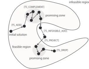
Computational procedure of tabu search for general 0-1 programming problems

Step 0: INITIALIZATION

Otherwise, go to step 1. Step 1: TS PROJECT

The aim of this step is to move the current solution in the infeasible region to the promising zone in the gen-tlest ascent (disimproving) direction about the objective function with decreasing the surplus of constraintsδ(x) While δ(x) is positive, i.e., the current solution is infeasible, repeat finding a non-tabu decision variable which decreasesδ(x) and gives the lest disimprovement of the objective function value when its value would be changed, changing the value of the decision variable ac-tually and adding the decision variable to TL. If there does not exist any non-tabu decision variable that de-creasesδ(x), select a decision variable randomly, change its value even ifδ(x) increases and add the decision vari-able to TL. If δ(x) = 0 and there does not exist any decision variable which improves the objective function value by changing its value, go to step 2.

Step 2: TS COMPLEMENT

The aim of this step is to search the promising zone intensively.

Let x0 := x and x00 := x0. Then, select several tabu decision variables of x00 and change their values. If δ(x00) = 0, then carry out step 4. Otherwise, carry out step 1. If f(x00)< f(x) for the solution δ(x00) ob-tained by step 4 or step 1, letx:=x00. This procedure is repeated D times. If the previous step of this step is step 1, then go to step 3. If the previous step of this step is step 4, then go to step 5.

Step 3: TS DROP

The aim of this step is to move the current solution in the promising zone to the inside of the feasible region in the gentlest ascent direction of the objective function with increasing the slackness of constraints(x)

Repeat finding a non-tabu decision variable which in-creases (x) and gives the lest disimprovement of the objective function when its value would be changed, changing the value of the decision variable actually and adding the decision variable to TL. If there does not exist any non-tabu decision variable that increases(x) or the number of repetitions of the above procedure ex-ceeds TT, go to step 4.

Step 4: TS ADD

The aim of this step is to move the current solution in the feasible region to the promising zone in the steepest descent (improving) direction about the objective func-tion with keepingδ(x) = 0.

Whileδ(x) = 0, i.e., the current solution is feasible, repeat finding a non-tabu decision variable which keeps

δ(x) = 0 and gives the greatest improvement of the ob-jective function value when its value would be changed, changing the value of the decision variable actually and adding the decision variable to TL. If there does not ex-ist such a decision variable, go to step 2.

Step 5: TS INFEASIBLE ADD

The aim of this step is to move the current solution in the promising zone to the infeasible region in the steepest descent (if exist) or the gentlest ascent direction about the objective function with decreasing the slackness of constraints(x) or increasing the surplus of constraints

δ(x).

Repeat finding a non-tabu decision variable which de-creasing the slackness of constraints (x) or increasing

the surplus of constraintsδ(x) and gives the greatest im-provement (if exist) or the lest disimim-provement of the ob-jective function value when its value would be changed, changing the value of the decision variable actually and adding the decision variable to TL. If there does not ex-ist such a decision variable or the number of repetitions of the above procedure exceeds Omax, return to step 1.

The search procedure of the proposed tabu search for general 0-1 programming problems is illustrated in Fig-ure 2

initial solution

feasible region

infeasible region

[image:6.595.348.500.183.301.2]

promising zone

[TS_ADD]

[TS_COMPLEMENT]

[TS_INFEASIBLE_ADD]

[TS_DROP] promising zone

[TS_PROJECT]

Figure 2. Tabu search for general 0-1 programming.

5

Numerical example

As an illustrative numerical example, consider the fol-lowing stochastic three-level 0-1 programming problem:

minimize DM1 (Level 1)

c11(ω)x1+c12(ω)x2+c13(ω)x3 minimize

DM2 (Level 2)

c21(ω)x1+c22(ω)x2+c23(ω)x3 minimize

DM3 (Level 3)

c31(ω)x1+c32(ω)x2+c33(ω)x3 subject to A1x1+A2x2+A3x3≤b(ω)

x1∈ {0,1}n1, . . . ,x3∈ {0,1}n3

                

(16)

where x1 = (x1, . . . , x15)T,x2 = (x16, . . . , x30)T,x3 = (x31, . . . , x45)T; each entry of 15-dimensional row con-stant vectors cij, i, j = 1,2,3, and each entry of 3×15

coefficient matricesA1, A2, andA3 are random

Through the use of this numerical example, it is now appropriate to illustrate the proposed interactive fuzzy programming method.

In step 1 of the interactive fuzzy programming, DM1 specifies satisficing levels αl, l = 1,2,3 and βi, i =

1,2, . . . ,9 as:

(α1, α2, α3)T = (0.75,0.75,0.75)T, (β1, β2, β3, β4, β5, β6, β7, β8, β9)T = (0.95,0.80,0.85,0.90,0.90,0.85,0.85,0.95,0.80)T_.

For the specified satisficing levels αl, l = 1,2,3 and

βi, i= 1,2, . . . ,9, in step 2, minimal values Zl,Fmin and

Z_l,MF of objective functions Z_lF(x1,x2,x3) under the chance constraints are calculated. By considering these values, the DMs identify the linear membership function whose parameter values are determined by the Zimmer-mann method [17].

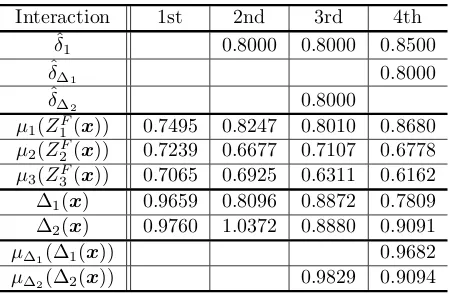
In step 3, the maxmin problem is solved. The obtain result is shown at the column labeled “1st” in Table 1.

[image:7.595.50.275.71.218.2]

Table 1. Interaction process

Interaction 1st 2nd 3rd 4th

ˆ

δ1 0.8000 0.8000 0.8500

ˆ

δ∆1 0.8000

ˆ

δ∆2 0.8000

µ1(ZF

1(x)) 0.7495 0.8247 0.8010 0.8680

µ2(Z2F(x)) 0.7239 0.6677 0.7107 0.6778

µ3(ZF

3(x)) 0.7065 0.6925 0.6311 0.6162 ∆1(x) 0.9659 0.8096 0.8872 0.7809 ∆2(x) 0.9760 1.0372 0.8880 0.9091

µ∆1(∆1(x)) 0.9682

µ∆2(∆2(x)) 0.9829 0.9094

Since DM1 is not satisfied with this solution, DM1 sets the minimal satisfactory level ˆδ1 to 0.80. (12) For ˆ

δ1= 0.80 (12) is solved, and the obtained optimal solu-tion is µ1(Z1F(x)) = 0.8247, µ2(Z2F(x)) = 0.6677, and

µ3(Z3F(x)) = 0.6925, as is shown at the column labeled “2nd” in Table 1.

In step 5, DM2 sets the membership function

µ∆2(∆2(x)) for the ratio ∆2 of satisfactory degrees

and the minimal satisfactory level as ˆδ∆2 = 0.80. For

ˆ

δ∆2 = 0.80 (13) is solved, and the obtained result is

shown at the column labeled “3rd” in Table 1. For the obtained optimal solution to (13), µ1(ZF

1(x)) = 0.8010, µ2(Z₂F(x)) = 0.7107, µ3(Z₃F(x)) = 0.6311 and

µ∆2(∆2(x)) = 0.9829.

In step 6, since the ratio of satisfactory degrees ∆2is greater than ˆδ∆2 = 0.80, the condition of termination of

the interactive process is fulfilled. Then, DM1 is asked whether he is satisfied with the obtained solution. Since DM1 is not satisfied, and he updates the minimal sat-isfactory level ˆδ1 from 0.80 to 0.85 in order to improve

µ1(Z₁F(x)) and sets ˆδ∆1= 0.80.

In step 7, (14) for ˆδ1 = 0.85 and ˆδ∆1 = 0.800 is

solved. The obtained result is shown at the column la-beled “4th” in Table 1. For the obtained optimal solu-tion to (14),µ1(Z1F(x)) = 0.8680,µ2(Z2F(x)) = 0.6778,

µ3(Z3F(x)) = 0.6162 andµ∆1(∆1(x)) = 0.9682.

In step 6, since the current solution satisfies all termi-nation conditions of the interactive process and DM1 is satisfied with the current solution, the satisfactory solu-tion is obtained and the interacsolu-tion procedure is termi-nated.

6

Conclusion

In this paper, with simultaneously considering uncer-tainty and discreteness often appeared in the real world hierarchical decision making situations, we first formu-lated multi-level 0-1 programming problems with ran-dom variable coefficients in both objective functions and constraints. Through the use of fractile models together with chance constrained programming, the formulated stochastic multi-level 0-1 programming problems were transformed into deterministic 0-1 programming ones. Considering the vague nature of the DMs’ judgments in the transformed multi-level 0-1 programming problems, interactive fuzzy programming has been proposed. In

the proposed interactive method, after determining the fuzzy goals of the DMs at all levels, a satisfactory so-lution is derived efficiently by updating the satisfactory degree of the DM at the 1st level with considerations of overall satisfactory balance among all levels. It is sig-nificant to note here that the transformed deterministic problems to derive an overall satisfactory solution can be effectively solved through the proposed tabu search for general 0-1 programming problems. An illustrative nu-merical example for a three-level 0-1 programming prob-lem was provided to demonstrate the feasibility of the proposed method. However, further computational ex-periences should be carried out for several types of nu-merical examples. From such experiences the proposed method must be revised. As a subject of future work, applications of the proposed method to the real world decision making situations should be considered in the near future. Extensions to other stochastic program-ming models will be considered elsewhere. Also exten-sions to multi-level 0-1 programming problems involving fuzzy random variable coefficients and/or random fuzzy coefficients will be required in the near future.

REFERENCES

[1] M. Sakawa, I. Nishizaki. Cooperative and Noncooper-ative Multi-Level Programming, Springer, New York, 2009.

[2] Y. J. Lai. Hierarchical optimization: a satisfactory solu-tion, Fuzzy Sets and Systems, Vol. 77, No. 3, 321–335, 1996.

[3] H. S. Shih, Y. J. Lai, E. S. Lee. Fuzzy approach for multi-level programming problems, Computers and Op-erations Research, Vol. 23, No. 1, 73–91, 1996.

[4] M. Sakawa, I. Nishizaki, Y. Uemura. Interactive fuzzy programming for multi-level linear programming prob-lems, Computers & Mathematics with Applications, Vol. 36, No. 2, 71–86, 1998.

[5] M. Sakawa, I. Nishizaki, Y. Uemura. Interactive fuzzy programming for two-level linear fractional program-ming problems with fuzzy parameters, Fuzzy Sets and Systems, Vol. 115, No. 1, 93–103, 2000.

[6] M. Sakawa, I. Nishizaki. Interactive fuzzy programming for decentralized two-level linear programming prob-lems, Fuzzy Sets and Systems, Vo. 125, No. 3, 301–315, 2002.

[7] M. Sakawa, I. Nishizaki, Y. Uemura. A decentral-ized two-level transportation problem in a housing material manufacturer –Interactive fuzzy programming approach–, European Journal of Operational Research, Vol. 141, No. 1, 167–185, 2002.

[8] M. Sakawa. Fuzzy multiobjective and multilevel opti-mization, In M. Ehrgott, X. Gandibleux (Eds.), Multi-ple Criteria Optimization –State of the art annotated bibliographic surveys–, Kluwer Academic Publishers, Boston, 171–226, 2002.

[10] M. Sakawa, H. Katagiri, T. Matsui. Interactive fuzzy random two-level linear programming through fractile criterion optimization, Mathematical and Computer Modelling, Vol. 54, 3153–3163, 2011.

[11] M. Sakawa, H. Katagiri, T. Matsui. Interactive fuzzy stochastic two-level integer programming through frac-tile criterion optimization, Operational Research: An International Journal, Vol. 12, pp. 209–227, 2012.

[12] M. Sakawa, T. Matsui. Interactive fuzzy program-ming for stochastic two-level linear programprogram-ming prob-lems through probability maximization, Artificial Intel-ligence Research, Vol. 2, 109–124, 2013.

[13] M. Sakawa, I. Nishizaki. Interactive fuzzy programming for multi-level programming problems: a review, Inter-national Journal of Multicriteria Decision Making, Vol. 2, No. 3, 241–266, 2012.

[14] I. M. Stancu-Minasian. Stochastic Programming with Multiple Objective Functions, D. Reidel Publishing Company, Dordrecht, 1984.

[15] I. M. Stancu-Minasian. Overview of different ap-proaches for solving stochastic programming prob-lems with multiple objective functions, In R. Slowin-ski, J. Teghem (Eds.), Stochastic Versus Fuzzy Ap-proaches to Multiobjective Mathematical Programming under Uncertainty, Kulwer Academic Publishers, Dor-drecht/Boston/London, 71–101, 1990.

[16] M. Sakawa, I. Nishizaki, H. Katagiri. Fuzzy Stochas-tic Multiobjective Programming, Springer, New York, 2011.

[17] H.-J. Zimmermann. Fuzzy programming and linear pro-gramming with several objective functions, Fuzzy Sets and Systems, Vol. 1, No. 1, 45–55, 1978.

[18] M. Sakawa. Fuzzy Sets and Interactive Multiobjective Optimization, Plenum Press, New York, 1993.

[19] M. Sakawa. Genetic Algorithms and Fuzzy Multi-objective Optimization, Kluwer Academic Publishers, Boston, 2001.

[20] G. B. Dantzig. Linear programming under uncertainty, Management Science, Vol. 1, No. 3–4, 197–206, 1955.

[21] A. Charnes, W. W. Cooper. Chance constrained pro-gramming, Management Science, Vol. 6, No. 1, 73–79, 1959.

[22] M. Sakawa, H. Yano, T. Yumine. An interactive fuzzy satisficing method for multiobjective linear-programming problems and its application, IEEE Transactions on Systems, Man and Cybernetics, Vol. SMC-17, No. 4, 654–661, 1987.

[23] M. Sakawa, Fuzzy multiobjective optimization, In M. Doumpos, E. Grigoroudis (Eds.), Multicriteria Deci-sion Aid and Artificial Intelligence: Links, Theory, and

Applications, John Wiley & Sons, New York, 235–271, 2013.

[24] M. Sakawa, K. Kato. An interactive fuzzy satisficing method for multiobjective stochastic linear program-ming problems using chance constrained conditions, Journal of Multi-Criteria Decision Analysis, Vol. 11, No. 3, 125–137, 2002.

[25] M. Sakawa, K. Kato, I. Nishizaki. An interactive fuzzy satisficing method for multiobjective stochastic linear programming problems through an expectation model, European Journal of Operational Research, Vol. 145, No. 3, 655–672, 2003.

[26] M. Sakawa, K. Kato, H. Katagiri. An interactive fuzzy satisficing method for multiobjective linear pro-gramming problems with random variable coefficients through a probability maximization model, Fuzzy Sets and System, Vol. 146, No. 2, 205–220, 2004.

[27] M. Sakawa, H. Yano. An interactive fuzzy satisficing method using augmented minimax problems and its ap-plication to environmental systems, IEEE Transactions on Systems, Man and Cybernetics, Vol. SMC-15, No. 6, 720–729, 1985.

[28] M. Sakawa, H. Yano. Interactive decision making for multiobjective nonlinear programming problems with fuzzy parameters, Fuzzy Sets and Systems, Vol. 29, No. 3, 315–326, 1989.

[29] M. Sakawa, H. Yano. An interactive fuzzy satisficing method for generalized multiobjective linear program-ming problems with fuzzy parameters, Fuzzy Sets and Systems, Vol. 35, No. 2, 125–142, 1990.

[30] M. Sakawa, K. Kato. Interactive fuzzy multi-objective stochastic linear programming, In C. Kahraman (Ed.), Fuzzy Multi-Criteria Decision Making –Theory and Ap-plications with Recent Developments–, Springer, New York, 375–408, 2008.

[31] A. Charnes, W. W. Cooper. Deterministic equivalents for optimizing and satisficing under chance constraints, Operations Research, Vol. 11, No. 1, 18–39, 1963.

[32] S. Kataoka. A stochastic programming model, Econometorica, Vol. 31, No. 1–2, 181–196, 1963.

[33] A. M. Geoffrion. Stochastic programming with aspira-tion or fractile criteria, Management Science, Vol. 13, No. 9, 672–679, 1967.

[34] S. Hanafi, A. Freville. An efficient tabu search approach for the 0-1 multidimensional knapsack problem, Euro-pean Journal of Operational Research, Vol. 106, No. 2–3, 659–675, 1998.