A New Approach for Dispersion Parameters

(1)

http://dx.doi.org/10.4236/jamp.2016.48165

A New Approach for Dispersion Parameters

Ahmed Mohamed Mohamed El-Sayed

Department of Management Information Systems, High Institute for Specific Studies, Nazlet Al-Batran, Giza, Egypt

Received 12 June 2016; accepted 19 August 2016; published 22 August 2016

This work is licensed under the Creative Commons Attribution International License (CC BY).

http://creativecommons.org/licenses/by/4.0/

Abstract

This paper presents a new approach to identify and estimate the dispersion parameters for biva-riate, trivariate and multivariate correlated binary data, not only with scalar value but also with matrix values. For this direction, we present some recent studies indicating the impact of over- dispersion on the univariate data analysis and comparing a new approach with these studies. Fol-lowing the property of McCullagh and Nelder [1] for identifying dispersion parameter in univa-riate case, we extended this property to analyze the correlated binary data in higher cases. Finally, we used these estimates to modify the correlated binary data, to decrease its over-dispersion, us-ing the Hunua Ranges data as an ecology problem.

Keywords

Measures of Association, Correlated Binary Data, Dispersion Parameters, Scaled Deviance, Scalar Value, Scalar Matrix

1. Introduction

The dispersion parameter should be the unity in case of the univariate Bernoulli data, but there may be deviation if there is a sequence of the Bernoulli outcomes included in a study that may lead to a binomial variable. The

over-dispersion is happened if the variance of actual response is more than the nominal variance, Var Y

( )

>V

( )

µ ,

as a function of the mean, µ. The estimation of dispersion parameter in the univariate case can be obtained

(2)

the univariate case. The estimate of dispersion parameters for the bivariate correlated binary data can be ob-tained using different methods. The first one when the dispersion parameter is scalar. The second one when we have a matrix values of dispersion parameters. These estimates can be extended to the trivariate and multivariate correlated binary data. So, we present a new approach to identify and estimate the dispersion parameters, in sca-lar and matrix values, for the bivariate, trivariate and multivariate correlated binary data. Also, after obtaining these estimates we can modify the correlated binary data, this happens to obtain a dispersion parameter equal or near to the unity.

This paper can be organized as follows: Some of the previous studies are presented in the Section 2.

A proposed approach for identifying and estimating the dispersion parameters in a scalar and matrix values, and the impact of over-dispersion in the case of bivariate, trivariate and multivariate binary outcomes associated with covariates, are demonstrated in the Sections 3, 4 and 5, respectively.

Finally, the numerical examples for the vectorized generalized additive model, VGAM, or vectorized

genera-lized linear model, VGLM, Yee and Wild [2], and the alternative quadratic exponential form, AQEF, measure,

El-Sayed et al. [3], are demonstrated in Section 6.

2. Previous Studies

In this section, we present some studies on the over-dispersion problem as shown below:

(1) Smith and Heitjan [4] provided an appropriate statistical tool to detect extra binomial variation (over-disp-

ersion). To test the nominal dispersion in the i-th (i=1, 2,,d) margin, it is important to give the relation, for

i

m trials,

( )

i i i i

(

1 i

)

.

Var Y =φ πm −π (1)

The hypothesis testing problem is formulated as

0: i 1 vs 1: i 1.

H φ = H φ >

An appropriate procedure to test H0 is the score statistic suggested by Smith and Heitjan

2 1

, i i i J A J χ ₌ _′ −

(2)

where Ji =

(

J1i,J2i,,Jpi

)

is a random vector that registers the difference between actual information and

no-minal information, in the i-th margin with respect to every j-th (j=1, 2,,p) parameter, for k k

(

=1, 2,,n

)

observations, namely

(

)

2

(

)

₂

. 1

1

1 ,

2

n

ji jik i i i i i jik

k

J y mπ mπ π x

=

 

=

∑

__ − − − __ (3)

And Ai is the covariance matrix of Ji corrected for estimation of linear predictors, θi, where

log 1

i i

i π θ

π =

− . Under the null hypothesis, H0, the asymptotic distribution of statistic (2) is the

2

χ distribution

with p degrees of freedom. The eventual rejection of H0 will be a clear evidence that Var Y

( )

i >miπi

(

1−πi

)

.

(2) Cook and Ng [5] described a bivariate logistic-normal mixture model for over-dispersed two state Markov

processes. The use of these mixed models cause increase in the standard error of marginal probability estimates. They did not specify the explicit form for the over-dispersion estimate, but display the log-likelihood function for the full sample of m subjects, as

(

)

(

) (

)

1 2

(

)

2

1 1

, log , | 1 , | ,

1, 2, , , 1, 2,

k i k i kli kli

i m

n n n

n

k ki k ki k ki k ki

i k

y E p x p x

i m k l

α

θ β α + − β α

= =

  

=   × − 

 

 

= ≠ =

∑

∏





(4)

where, the expectation, Eα_i, is taken with respect to the bivariate normal distribution, hence

(

1, 2

)

~

(

,

)

i i i BVN

(3)

(3) Saefuddin et al. [6] showed the effect of over-dispersion on the hypothesis test of logistic regression.

A simple method proposed by William, [7], was used to correct the effect of over-dispersion by taking

infla-tion factor into considerainfla-tion. This method takes account of adjusting the estimate of the standard error of the parameter resulting from the over-dispersion. Modeling of the over-dispersion is often expressed in the equation of the variance of response variable, Yi, for binomial case for ni trials, as follows

( )

i i i

(

1 i

)

1

(

i 1

)

,

Var Y =nπ −π _ + n − φ_ (5)

where 1+

(

ni−1

)

φ is the over-dispersion scale and φ denote inflation factor. When the over-dispersion

does not occur or very small over-dispersion occurs, φ will be approximately equal to zero, so Yi exactly

follows binomial distribution, Bin n

(

i,πi

)

, and Var Y

( )

i =niπi

(

1−πi

)

, Collett [8]. However, when over-dis-

persion exists, φ exceeds zero and leads Var Y

( )

i to be greater than niπi

(

1−πi

)

. The parameter estimate of

φ, is obtained by equating X2 statistic of the model to its approximate expected value, written as

(

)

(

)

( )

(

)

(

)

2

2 2

1 1

ˆ

, and 1 1 1 ,

ˆ 1 ˆ

n n

i i i i

i i i i i

w y n

X E X w w d n

n

π

υ φ

π π

= =

−

 

= − _ + − _

−

∑



∑

(6)

where υ_i=n_iπ_i

(

1−π_i

)

, wi is the weight and di is the diagonal element of the variance-covariance matrix of

the linear predictor, say ˆ_i p₁ˆ_j _ji

j x

η =

∑

₌β . The value of X2 statistic depends on ˆφ, so iteration process is

needed to find the optimum value. This procedure was the first introduced by William, [7], and is known as

Wil-liam method.

The algorithm of the William method is described as follows:

1. Assume φ =0, calculate parameter estimate of logistic regression parameter, ˆβ, using maximum

like-lihood method. Calculate the X2 statistics of fitted model.

2. Compare X2 statistics to 2

n p

χ₋ distribution. If X2 statistic is too large, conclude that φ >0 and

cal-culate the initial estimates of φ using following formula

(

)

(

)(

)

2 0

1

ˆ _.

1 1

i n

i i i

i

X n p

n d

φ

υ =

− −

=

− −

∑

(7)

3. Using the initial weights

(

)

1

0i 1 i 1 ˆ0 ,

w = +_ n − φ _− (8)

we can recalculate the value of βˆ and X2 statistic.

4. If X2 statistic close to its degrees of freedom, n−p, then the estimated value of φ is sufficient. If not,

re-estimate φ using following expression:

(

)

(

)(

)

2 1

1

ˆ _.

1 1

n

i i i i

i n

i i i i i

i

X w w d

w n w d

υ φ

υ =

=

− −

=

− −

∑

(9)

If X2 statistic remains large, return to step (3) until optimum value of estimated φ is obtained. Once φ

has been estimated by φˆ, wi 1

(

ni 1

)

φ 1

−

 

= +_ − _ could be used as weights in fitting the new model, Collett [8],

and William [7]. We conclude that the over-dispersion problem causes lower standard errors of the estimates of

parameters.

(4) Davila et al. [9] introduced a new approach for modeling the multivariate marginals over-dispersed

bi-nomial data. They illustrate this approach by analyzing the data using the Gaussian copula with Beta-bibi-nomial margins. In order to model the over-dispersion, they used the Beta-binomial model, a generalization of binomial

distribution, Casella and Berger [10]. In this model, it is supposed that Y Pi| i~Bin m P

(

i, i

)

, whereas

(

)

~ ,

i i i

P Beta α β . Then, they make the assumption that each margin, Yi, follows a Beta-binomial distribution.

(4)

(

)

(

₍

,

₎

)

{

}

, , , 0,1, , ,

,

i i i i i i

i i i i i

i i i

m Beta y m y

f y y m

y Beta

α β

+ − +

 

=_ _ ∈

   (10)

where, αi >0,βi >0. Conditional to Pi, the expectation is given by

(

|

)

i , 1, 2, , ,

i i i i i

i i

E Y P mπ m α i d

α β

 

= = _ _ =

+

   (11)

The conditional variance is

(

|

)

(

1

)

(

1

)

1

(

1 ,

)

1, 2, , .

1

i i i

i i i i i i i i i i

i i

m

Var Y P mπ π α β mπ π φ m i d

α β

+ +

 

= − = − _ + − _ =

+ +  (12)

From the relation (12), we see that the marginal dispersion parameter is

1 . 1

i

i i

φ

α β

=

+ + (13)

Comparing the relation (1) with the relation (12), it is noted that the later has a greater variance. In their study, as compared with the multivariate normal (MVN), the marginal GLM, and the marginal over-dispersion model (ODM), they have shown that the model based on the Beta-binomial model (BBM) displayed the higher stan-dard errors associated to estimated parameters.

(5)-The vectorized generalized additive model (VGAM) introduced by Yee and Wild [2] and implemented by

Yee [11] [12]. The conditional distribution of VGAM function for bivariate correlated binary responses,

(

Y Y1, 2

)

given that some covariates, x, is:

(

1 2

)

0

( )

1

( )

1 2

( )

2 12

( )

1 2

logf y y, |x =u x +u x y +u x y +u x y y , (14) where, u0

( )

x is the normalizing constant,

( )

1 1

2 2

12 3

,

u x x

u x x x

u x x

η

η η

η

   

 ₌ ₌ 

   

   

And the ηj, j=1, 2, 3, are additive predictors. If all the functions are constrained to be linear, then the

re-sulting model is a vector generalized linear model (VGLM).

The conditional distribution of VGAM family function for trivariate binary responses,

(

Y Y Y1, 2, 3

)

given that

some covariates, x, is

(

1 2 3

)

0

( )

1

( )

1 2

( )

2 3

( )

3 12

( )

1 2 13

( )

1 3 23

( )

2 3

logf y y y, , |x =u x +u x y +u x y +u x y +u x y y +u x y y +u x y y . (15) Note that a third order association parameter, u123, for the product,

(

y y y1 2 3

)

, is assumed to be zero for this

family, Yee and Wild [2].

The conditional distribution of VGAM (VGLM) function for multivariate correlated binary responses,

(

Y Y Y1, 2, 3,,Yk

)

, given that some covariates, x, is

(

1 2

)

0

( )

1

log , , , | ,

k k

k j j jl j l

j j l

f y y y x u x u x y u x y y

= <

= +

∑

+

∑

 (16)

where u0

( )

x is the normalizing constant.

In the next section, we suggest a new approach to estimate the dispersion parameter, φ, using a scalar and a

matrix values of the dispersion parameters and indicate how the dispersion parameter may influence on the analysis of correlated binary data, specially on the standard errors, the Wald statistics and the LRTs for the biva-riate, trivariate and multivariate binary outcomes variables associated with covariates. For fitting the correlated binary data, we use the log-likelihood function for the alternative quadratic exponetial form (AQEF) measure,

[3], in the bivariate, trivariate and multivariate case, respectively.

(5)

(

)

( )

(

)

(

)

( )

(

)

( )

(

)

(

)

(

)

(

)

1

2

3

1 10 11 1 1

2 20 21 2 2

3 30 31 3 3

1 10 11

2 20 21

3 30 31

4 40 41

e

, , 1 , 1, 2, , ,

1 e

e

, ,

1 e e

, ,

1 e ,

,

x

i x

x

x p x x x i n

x p x

β

β β β µ

α α α

′ ′ ′ ′ ′

′



′= = = ′= = _

+ _



′ = = = _

+ _



′ = = = _

+



′ = _



′ = _

 ′ =



′= _



(17)

we have the log-likelihood function for the bivariate AQEF measure as

(

)

(

1 2 1 2

)

1 2 1 1 2 2 1 2 1

, , , log 1 e e e .

n

x x x x x

i i i i

i

y β β α β xy β xy α xy y β′ β′ β′+β′ +α′

=

 ′ ′ ′ 

=

∑

_ + + − + + + _

 (18)

The log-likelihood function for the trivariate AQEF measure is

(

y, ,β α

)

=β1′xy1+β2′xy2+β3′xy3+α1′xy y1 2+α2′xy y1 3+α3′xy y2 3+α′4xy y y1 2 3−logA

(

β α,

)

,

 (19)

where,

(

_,

)

_{1 e}1x _e2x _e3x _e1x 2x 1x _e1x 3x 2x _e2x 3x 3x _e1x 2x 3x 1x 2x 3x 4x

A β α = + β′ + β′ + β′ + β′+β′ +α′ + β′+β′+α′ + β′ +β′ +α′ + β′+β′ +β′+α′+α′ +α′ +α′

Finally, the log-likelihood function for the multivariate AQEF measure is

(

)

12 1 2

(

)

1 1 1

, , log , ,

n k k

j ji jl ji li k i i ki

i j j l

y β α β xy α xy y α xy y y A β α

= = ≤ <

 

′ ′ ′

= _ + + + − _

 

∑ ∑

∑



   (20)

where,

(

)

( )

123

1 1 1

, 1 exp exp exp .

k k k

j j l jl j k

j j l j

A β α β x β x β x α x β x α x

= ≤ < =

 

′ ′ ′ ′ ′ ′

   

= + _ _+ _ + + _+ + _ + + _

 

∑



∑

  (21)

3. Dispersion Parameters in Bivariate Case

In this section, we determine the identification and estimation of a fixed value for dispersion parameter, φ, and

also a matrix of dispersion parameters to extend the effect of over-dispersion on the analysis of bivariate corre-lated binary data.

3.1. Scalar Dispersion Parameter

We can use the variance-covariance matrix of Y1 and Y2 to estimate a scalar dispersion parameter, φ, in the

bivariate binary outcomes. So, we can define the response vector

1 2 Y Y

Y

  =  

  and its mean vector

1 2 Y Y

Y

  =  

 .

Following the GLM property, the variance-covariance matrix of Y is

( )

(

)

(

)

( )

11 12 1 1 2

21 22 2 1 2

, , ,

V V

σ σ µ µ µ

φ

σ σ µ µ µ

 

Σ =_ __{= } _

   

where,

(

)

2

(

)

2

(

)(

)

11 E Y1 1 , 22 E Y2 2 , 12 21 E Y1 1 Y2 2 ,

(6)

And,

( )

1 1

(

1 1

)

,

( )

2 2

(

1 2

)

,

(

1, 2

)

(

2, 1

)

12

( ) ( )

1 2 ,

V µ =µ −µ V µ =µ −µ Cov µ µ =Cov µ µ =ρ V µ V µ

Then, the estimator of φ, for n observations, is

[

]

₍

( )

1

₎

(

_{( )}

1 2

)

1 1 1

1 1 2 2

1 2 1 2 2 2

ˆ

ˆ ˆ , ˆ

1

ˆ _ˆ _ˆ _.

ˆ

ˆ ,ˆ ˆ

n

i i

i i i

i i i i

i i i i i i

y V Cov y y y Cov V n p µ

µ µ µ

φ µ µ

µ

µ µ µ

−

=

   − 

= − − _ _{ } _

−

∑

_ _ _ _ (22)

Hence, we can show that

(

) ( ) (

) ( )

(

)(

)

( ) ( )

(

)

2 2

1 1 2 2 2 1 1 2 1 1 2 2

2 1

1 2 1 2

ˆ ˆ ˆ ˆ 2 ˆ , ˆ ˆ ˆ

1

ˆ _.

ˆ ˆ ˆ , ˆ

n

i i i i i i i i i i i i

i

i i i i

y V y V Cov y y

n p _V _V _Cov

µ µ µ µ µ µ µ µ

φ

µ µ µ µ

=

− + − − − −

=

−

∑

_{− }_ __ (23)

Then,

[

]

₍

( )

1

₎

(

_{( )}

1 2

)

1 1 1

1 1 2 2

1 2 1 2 2 2

, ,

n

i i

i i i

i i i i

i i i i i i

y V Cov y y y Cov V µ

µ µ µ

µ µ

µ

µ µ µ

− =    −  − − _ _{ } _ −    

∑

Follows the non-central 2

n p

χ ₋ . Under independence, this quantity follows, approximately, 2

n p

χ ₋ . An

estima-tor of φ in this case is

(

)

(

)

(

)

2 2

1 1 2 2

1 1 1 2 2

ˆ ˆ

1

ˆ _.

ˆ 1 ˆ ˆ 1 ˆ

n

i i i i

i i i i i

y y

n p

µ µ

φ

µ µ µ µ

=

 ₋ ₋ 

=  + 

−

∑

__ − − __ (24)

3.2. Matrix of Dispersion Parameters

Now, we use different values for dispersion parameter, such that φ φ φ11, 22, 12 and φ21, here, φ12 =φ21. The

va-riance-covariance matrix of Y is

( )

(

)

(

)

( )

11 12 11 1 12 1 2 21 22 21 2 1 22 2

, . ,

V V

σ σ φ µ φ µ µ

σ σ φ µ µ φ µ

 

Σ =_ __{= } _

    (25)

The estimator of dispersion parameters matrix is

( )

(

)

(

)

( )

11 12

1 1 2

11 12

21 22

2 1 2

ˆ ˆ

ˆ ˆ ˆ ˆ,ˆ

,

ˆ ˆ ˆ ˆ

ˆ , ˆ ˆ

V Cov

Cov V

σ σ

µ µ µ

φ φ

σ σ

φ φ

µ µ µ

        =   _ _    _{ } _   Then,

(

)

( )

(

)(

)

(

)(

)

(

)

(

( )

)

2

1 1 1 1 2 2

1 1 1 1 2

11 12

2

21 22 2 2 1 1 2 2

1 2 1 1 2

ˆ ˆ ˆ

ˆ ˆ ₁ ˆ ˆ ,ˆ

.

ˆ ˆ _ˆ _ˆ _ˆ

ˆ ,ˆ ˆ

n n

i i i i i i

j i j i i

n n

i i i i i i

j i i j i

y y y

V Cov

n p _y _y _y

Cov V

µ µ µ

φ φ

φ φ µ µ µ

µ µ µ

= = = =  ₋ ₋ ₋      _ _ =   ₋ _ _   − − −        

∑

(26)

From the equation (26), we have

[

]

₍

( )

₎

(

_{( )}

)

1

1 1 11 1 12 1 2

1 1 2 2

1 21 2 1 22 2 2 2

, ,

n

i i

i i i i i

i i i i

i i i i i i i i

y V Cov y y y Cov V µ

φ µ φ µ µ

µ µ

µ

φ µ µ φ µ

− =    −  − − _ _{ } _ −    

∑

Follows the non-central χn p2− . Under independence, this quantity follows, approximately,

2

n p

χ − . If

12 21

ˆ ˆ ₀

φ =φ = , and φˆ11=φˆ22=φˆ, then the estimator of φ is same as (24).

We can correct the data using the estimates of dispersion parameters, φ φˆ11,ˆ22, and Equation (25), for the i-th

(7)

( )

(

)

(

)

(

)

1

1 11 1 1

11

2

2 22 2 2

22

1 2

1 2 12 1 2 1 2

11 22

( ) ,

, , , , .

i

i i i i

i

i i i i

i

i i

i i i i i i i

i i

Y

Var Y V Var V

Y

Var Y V Var V

Y Y

Cov Y Y Cov Cov Cov

φ µ µ

φ

φ µ µ

ϕ

φ µ µ µ µ

φ φ



  _

= ⇔ _ _=



  _



= ⇔ = 

 

  _

= ⇔ _ _= _

  

(27)

4. Dispersion Parameters in Trivariate Case

We can define the response vector

1 2 3 Y Y Y Y

    =      

and its mean vector

1 2 3 µ

µ µ

µ     =      

.

The variance-covariance matrix of Y can be written as

( )

(

)

(

)

(

)

(

)

(

)

(

)

( )

11 12 13 1 1 2 1 3

21 22 23 2 1 2 2 3

31 32 33 3 1 3 2 3

, ,

= = , ( ) , ,

, ,

V Cov Cov

Cov V Cov

Cov Cov V

σ σ σ µ µ µ µ µ

 

 

Σ _ _ _ _

 

   

(28)

where,

( )

(

)

( )

(

)

( )

(

)

(

)

( ) ( )

(

)

( ) ( )

(

)

( ) ( )

1 1 1 2 2 2 3 3 3

1 2 12 1 2 1 3 13 1 3 2 3 23 2 3

1 , 1 , 1 ,

, , , , , .

V V V

Cov V V Cov V V Cov V V

µ µ µ µ µ µ µ µ µ

µ µ ρ µ µ µ µ ρ µ µ µ µ ρ µ µ

= − = − = −

= = =

The estimator of φ, for n observations, is

[

]

(

( )

)

(

( )

)

(

)

(

)

(

)

( )

1

1 1 2 1 3 1 1

1 1 2 2 3 3 2 1 2 2 3 2 2

1

3 1 3 2 3 3 3

ˆ ˆ ,ˆ ˆ ,ˆ ˆ

1

ˆ _ˆ _ˆ _ˆ _ˆ _,_ˆ _ˆ _ˆ _,_ˆ _ˆ _.

ˆ ,ˆ ˆ ,ˆ ˆ ˆ

i i i i i i i

n

i i i i i i i i i i i i i

i

i i i i i i i

V V V y

y y y V V V y

n p

V V V y

µ µ µ µ µ µ

φ µ µ µ µ µ µ µ µ µ

µ µ µ µ µ µ

−

=

   − 

   

= − − − _ _{ } − _

− _ _{ } _

−

 

∑

(29)

Since,

[

]

(

( )

)

(

( )

)

(

)

(

)

(

)

( )

1

1 1 2 1 3 1 1

1 1 2 2 3 3 2 1 2 2 3 2 2

=1

3 1 3 2 3 3 3

, ,

i i i i i i i

n

i i i i i i i i i i i i i

i

i i i i i i i

V Cov Cov y

y y y Cov V Cov y

Cov Cov V y

µ µ µ µ µ µ

−

   − 

   

− − − _ _{ } − _

  _ − _

 

∑

n p

χ − . Then, under independence, this quantity follows, approximately, χn p2− . Under

independence, the estimator of φ is

(

)

(

)

(

)

(

)

2 2 2

1 1 2 2 3 3

1 1 1 2 2 3 3

ˆ ˆ ˆ

1

ˆ _.

ˆ 1 ˆ ˆ 1 ˆ ˆ 1 ˆ

n

i i i i i i

i i i i i i i

y y y

n p

µ µ µ

φ

µ µ µ µ µ µ

=

 ₋ ₋ ₋ 

=  + + 

−

∑

__ − − − __ (30)

The variance-covariance matrix of Y can be displayed as

( )

(

)

(

)

(

)

( )

(

)

(

)

(

)

( )

11 12 13 11 1 12 1 2 13 1 3 21 22 23 21 2 1 22 2 23 2 3 31 32 33 31 3 1 32 3 2 33 3

, ,

, , .

, ,

V Cov Cov

Cov V Cov

Cov Cov V

σ σ σ φ µ φ µ µ φ µ µ

σ σ σ φ µ µ φ µ φ µ µ

σ σ σ φ µ µ φ µ µ φ µ

 

 

Σ =_ __{= } _

 

   

(8)

The estimator of dispersion parameters,

11 12 13

21 22 23

31 32 33

ˆ ˆ ˆ

φ φ φ

            , are

(

)

( )

(

)(

)

(

)(

)

(

)(

)

(

)

(

( )

)

(

)(

)

(

)(

)

2

1 1 1 1 2 2 1 1 3 3

1 1 1 1 2 1 1 3

2

2 2 1 1 2 2 2 2 3 3

1 2 1 1 2 1 2 3

3 3 1 1

1

ˆ ˆ ˆ ˆ ˆ

ˆ ˆ ,ˆ ˆ , ˆ

ˆ ˆ ˆ ˆ ˆ

1 ˆ

ˆ ,ˆ ˆ ˆ , ˆ

ˆ ˆ

n n n

i i i i i i i i i i

i i i i i i i i

n n n

i i i i i i i i i i

i i i i i i i i

n

i i i i

i

y y y y y

V Cov Cov

y y y y y

n p Cov V Cov

y y

Co

µ µ µ µ µ

φ

µ µ µ µ µ

µ µ = = = = = = = − − − − − − − − − − = − − −

∑

₍

₎

(

3 3

₍

)(

2

₎

2

)

(

3

_{( )}

3

)

2

1 1

3 1 3 2 3

.

ˆ ˆ ˆ

ˆ , ˆ ˆ ,ˆ ˆ

n n

i i i i i i

i i

i i i i i

y y y

v Cov V

µ µ µ

µ µ = µ µ = µ

               ₋ ₋ ₋      

∑

 (32) Since,

[

]

(

( )

)

(

( )

)

(

)

(

)

(

)

( )

1

11 1 12 1 2 13 1 3 1 1 1 1 2 2 3 3 21 2 1 22 2 23 2 3 2 2 =1

31 3 1 32 3 2 33 3 3 3

, ,

i i i i i i i i i i

n

i i i i i i i i i i i i i i i i

i

i i i i i i i i i i

V Cov Cov y

y y y Cov V Cov y

Cov Cov V y

φ µ φ µ µ φ µ µ µ

µ µ µ φ µ µ φ µ φ µ µ µ

φ µ µ φ µ µ φ µ µ

−    −      − − − _ _{ } − _   _ − _  

∑

n p

χ − . Under independence, this quantity follows, approximately, χn p2− . If

12 13 23

ˆ ˆ ˆ ₀

φ =φ =φ = and φˆ11=φˆ22=φˆ33=φˆ, then the estimator of φ is same as (30).

Similarly, we can correct the data using the estimates of dispersion parameters, φ φˆ11,ˆ22 and φˆ33, and the

eq-uation (31), for the i-th observation, in the trivariate case as

( )

(

)

(

)

(

)

1

1 11 1 1

11 2

2 22 2 2

22 3

3 33 3 3

33

1 2

1 2 12 1 2 1 2

11 22

1 3 13

, , , , ( , ) , , , , i

i i i i

i

i i i i

i

i i i i

i

i i

i i i i i i i

i i

Y

Var Y V Var V

Y

Var Y V Var V

Y

Var Y V Var V

Y Y

Cov Y Y

φ µ µ

φ

φ µ µ

φ

φ µ µ

φ

φ µ µ µ µ

φ φ φ   = ⇔ _ _=     = ⇔ _ _=     = ⇔ _ _=     = ⇔ _ _=   =

(

)

(

)

(

)

1 3

1 3 1 3

11 33 2 3

2 3 23 2 3 2 3

22 33

( , ) , , ,

, ( , ) , , .

i i

i i i i i

i i

i i i i i i i

i i

Y Y

Cov Cov Cov

Y Y

µ µ µ µ

φ φ

φ µ µ µ µ

φ φ                   _ ⇔ _ _= _   _     = ⇔ _ _=     (33)

5. Dispersion Parameters in Multivariate Case

We can define the response vector

1 2 k Y Y Y Y       =      

 and its mean vector

(9)

The variance-covariance matrix of Y can be written as

( )

(

)

(

)

(

)

( )

(

)

(

)

(

)

( )

11 12 1 1 1 2 1

21 22 2 2 1 2 2

1 2 1 2

, , , , , , , k k k k

k k kk k k k

V Cov Cov

Cov V Cov

Cov Cov V

σ σ σ µ µ µ µ µ

           

Σ = _{= } _

                          (34) where,

( )

(

)

(

)

( )

(

)

(

)

( ) ( )

(

)

( ) ( )

(

)

(

) ( )

1 1 1 2 2 2

1 2 12 1 2 1 3 13 1 3 1 1, 1

1 , ( ) 1 , , 1 ,

, , , , , , .

k k k

k k k k k k

V V V

Cov V V Cov V V Cov V V

µ µ ρ µ µ µ µ ρ µ µ µ− µ ρ − µ− µ

= − = − = −

= = =



The estimator of

φ

, for

n

observations, is

[

]

( )

(

)

(

)

(

)

( )

(

)

(

)

(

)

( )

1 1 1

1 1 2 1

2 2

2 1 2 2

1 1 2 2 1

1 2

ˆ

ˆ ˆ ,ˆ ˆ , ˆ

ˆ

ˆ ,ˆ ˆ ˆ , ˆ

1

ˆ _ˆ _ˆ _ˆ _.

ˆ

ˆ ,ˆ ˆ ,ˆ ˆ

i i

i i i i ki

n

i i

i i i i ki

i i i i ki ki

i

ki ki

ki i ki i ki

y

V V V

y

V V V

y y y

n p

y

V V V

µ

µ µ µ µ µ

µ

µ µ µ µ µ

φ µ µ µ

µ

µ µ µ µ µ

− =    −     ₋      = − − − _ _{ }  −    ₋       

∑

         (35) Since,

[

]

( )

(

)

(

)

(

)

( )

(

)

(

)

(

)

( )

1 1 1

1 1 2 1

2 2

2 1 2 2

1 1 2 2 =1 1 2 , , , , .. . , , i i

i i i i ki

n

i i

i i i i ki

i i i i ki ki

i

ki ki

ki i ki i ki

y

V V V

y

V V V

y y y

y

V V V

µ

µ µ µ µ µ

µ

µ µ µ µ µ

µ µ µ

µ

µ µ µ µ µ

−    −     ₋      − − − _ _{ }     ₋       

∑

       

Follows non-central 2

n p

χ − . Then, under independence, this quantity follows, approximately, χn p2− . Under

independence, the estimator of φ is

(

)

(

)

(

)

(

)

(

)

2 2 2 2

1 1 2 2 3 3

1 1 1 2 2 3 3

ˆ ˆ ˆ ˆ

1

ˆ _.

ˆ 1 ˆ ˆ 1 ˆ ˆ 1 ˆ ˆ 1 ˆ

n

i i i i i i ki ki

i i i i i i i ki ki

y y y y

n p

µ µ µ µ

φ

µ µ µ µ µ µ µ µ

=

 ₋ ₋ ₋ ₋ 

=  + + + + 

−

∑

__ − − −  − __ (36)

The variance-covariance matrix of Y can be displayed as

( )

(

)

(

)

(

)

( )

(

)

(

)

(

)

( )

11 12 1 11 1 12 1 2 1 1

21 22 2 21 2 1 22 2 2 2

1 2 1 1 2 2

, ,

.

, ,

k k k

k k kk k k k k kk k

V Cov Cov

Cov V Cov

Cov Cov V

σ σ σ φ µ φ µ µ φ µ µ

σ σ σ φ µ µ φ µ φ µ µ

σ σ σ φ µ µ φ µ µ φ µ

           

Σ = _{= } _

                          (37)

The estimator of dispersion parameters,

11 12 1 21 22 2

1 2

ˆ ˆ ˆ

k

k k kk

φ φ φ

(10)

(

)

( )

(

)(

)

(

)(

)

(

)(

)

(

)

(

( )

)

(

)(

)

(

)

2

1 1 1 1 2 2 1 1

1 1 1 1 2 1 1

2

2 2 1 1 2 2 2 2

1 2 1 1 2 1 2

1

ˆ ˆ ˆ ˆ ˆ

ˆ ˆ ,ˆ ˆ ,ˆ

ˆ ˆ ˆ ˆ ˆ

1

ˆ _ˆ _, _ˆ _ˆ _ˆ _,_ˆ

ˆ

n n n

i i i i i i i i ki ki

i i i i i i i ki

n n n

i i i i i i i i ki ki

i i i i i i i ki

n

ki ki i

i

y y y y y

V Cov Cov

y y y y y

Cov V Cov

n p

y y

µ µ µ µ µ

φ µ µ µ µ µ

µ = = = = = = = − − − − − − − − − − = − − −

∑

     

(

)

(

)

(

)(

)

(

( )

)

2

1 2 2

1 1

1 2

.

ˆ ˆ ˆ ˆ

ˆ ,ˆ ˆ ,ˆ ˆ

n n

i ki ki i i ki ki

i i

ki i ki i ki

y y y

Cov Cov V

µ µ µ µ

µ µ = µ µ = µ

                  − − −     

∑



∑

 (38) Since,

[

]

( )

(

)

(

)

(

)

( )

(

)

(

)

(

)

( )

1 1 1

11 1 12 1 2 1 1

2 2

21 2 1 22 2 2 2

1 1 2 2 =1

1 1 2 2

, ,

i i

i i i i i ki i ki

n

i i

i i i i i ki i ki

i i i i ki ki

i

ki ki

k i ki i k i ki i kki ki

y

V Cov Cov

y

Cov V Cov

y y y

y

Cov Cov V

µ

φ µ φ µ µ φ µ µ

µ

φ µ µ φ µ φ µ µ

µ µ µ

µ

φ µ µ φ µ µ φ µ

−    −     ₋      − − − _ _{ }     ₋       

∑

        

Follows non-central 2

n p

χ − . Under independence, this quantity follows, approximately, χn p2− . If

12 13 1,

ˆ ˆ ˆ ₀

k k

φ =φ =_=φ₋ = and φˆ11=φˆ22==φˆkk =φˆ, then the estimator of φ is same as (36). Similarly, we

can correct the data using the estimates of dispersion parameters, φ φˆ11,ˆ22,,φˆkk, and the equation (37), for the

i

-th observation, in the multivariate case as

( )

(

)

(

)

(

)

(

)

1

1 11 1 1

11 2

2 22 2 2

22

1 2

1 2 12 1 2 1 2

11 22

1 3 13

, , , , , , , , , i

i i i i

i

i i i i

i

ki

ki kki ki ki

kki

i i

i i i i i i i

i i

i i i

Y

Var Y V Var V

Y

Var Y V Var V

Y

Var Y V Var V

Y Y

Cov Y Y

φ µ µ

φ

φ µ µ

φ

φ µ µ

φ

φ µ µ µ µ

φ φ φ   = ⇔ _ _=     = ⇔ _ _=     = ⇔ _ _=     = ⇔ _ _=   = 

(

)

(

)

(

)

(

)

(

)

1 3

1 3 1 3

11 33

1,

1, 1, , 1, 1,

1, 1,

, , , ,

, , , , .

i i

i i i i

i i

k i ki

k i ki k k i k i ki k i ki

k k i kki

Y Y

Cov Cov Cov

Y Y

Cov Y Y Cov Cov Cov

µ µ µ µ

φ φ

φ µ µ µ µ

φ φ − − − − − − −                    _ ⇔ _ _= _   _     _   = ⇔ = _   _     (39)

6. Numerical Examples

In this section, we present two examples. The first one applies to the bivariate correlated binary data. This ex-ample presents the results obtained by using AQEF measure and the VGLM measure which are similar in the bivariate case. The second one applies on the trivariate binary data. However, the third association is absent in

the VGAM (VGLM) measure. In both examples, we will use the Hunua Ranges data, Yee [11] [12]. These data

were collected from the Hunua Ranges, a small forest in the Southern Auckland, New Zealand.

At 392 sites in the forest, the presence/absence of 17 plant species was recorded along with the altitude.

(11)

continuous variable, and there are binary responses (presence = 1, absence = 0) for 17 plant species. These data frame contains the following columns: agaaus, beitaw, corlae, cyadea, cyamed, daccup, dacdac, eladen, hedarb, hohpop, kniexc, kuneri, lepsco, metrob, neslan, rhosap, vitluc and altitude (meters above the sea level).

6.1. Application to Bivariate Case

Hence, we will use the first two columns, agaaus and beitaw, as correlated binary outcome variables, Y1 and

2

Y , respectively. A third column, corlae, is used as the explanatory binary variable, X.

We will use the estimates, φˆ11 and φˆ22, to modify the correlated data according to the relationship (27).

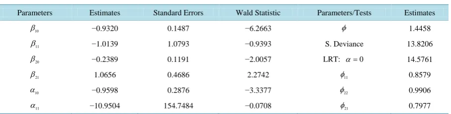
FromTable 1 andTable 2, we demonstrate the conclusions after modifying the correlated data by the esti-mates of dispersion parameters, as follows:

1. The estimates of the regression parameters are changed.

2. The standard errors are decreased for the estimates of association parameters. This leads to a significant association between the two outcomes binary variables,

(

Y Y1, 2

)

, associated with covariate, x.

3. The Wald statistic test shows lower values, this confirms a significant association between the two out-comes binary variables,

(

Y Y1, 2

)

, associated with covariate, x.

4. The LRT is increased, this also confirms the conclusion observed from the Wald statistic.

5. The estimate of a scalar dispersion parameter, φ, is increased.

6. The estimates of the matrix of dispersion parameters, φ φ11, 22 and φ12, increased and close to the unity.

7. The scaled deviance value is increased.

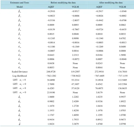
6.2.Application to Trivariate Case

We will use the columns, cyadea, beitaw and kniexc, as the dependent correlated binary variables, Y Y1, 2 and

3

Y , respectively. On the other hand, we will use the column “altitude”, meters above sea level, as the continuous

explanatory variable, X. The estimates of the regression parameters and their tests for the association parameters

[image:11.595.88.542.433.548.2]

can be determined for the AQEF and VGLM measures, before and after modifying the correlated data by the es-timates of dispersion parameters, φ φ11, 22 and φ33, as shown inTable 3.

Table 1. Results of AQEF and VGLM before modifying the data.

Parameters Estimates Standard Errors Wald Statistic Parameters/Tests Estimates

10

β −0.9320 0.1487 −6.2663 φ 1.4458

11

β −1.0139 1.0793 −0.9393 S. Deviance 13.8206

20

β −0.2389 0.1191 −2.0057 LRT: α =0 14.5761

21

β 1.0656 0.4686 2.2742 φ11 0.8579

10

α −0.9598 0.2876 −3.3377 φ22 0.9906

11

α −10.9504 154.7484 −0.0708 φ21 0.7977

Hence, the LRT’s will be compared with 2( )

0.05,1 = 3.8415

χ . Log-likelihood = −454.1039.

Table 2. Results of AQEF and VGLM after modifying data.

Parameters Estimates Standard Errors Wald Statistic Parameters/Tests Estimates

10

β ₋0.8212 0.1456 −5.6397 φ 1.4748

11

β −1.0256 1.0457 −0.9808 S. Deviance 26.5973

20

β −0.2106 0.1203 −1.7503 LRT: α=0 16.1546

21

β 1.0645 0.4720 2.2552 φ11 0.9549

10

α −0.9820 0.2788 −3.5225 φ22 1.0853

11

α ₋10.9610 149.3405 −0.0734 φ21 0.8361

Hence, the LRTs will be compared with 2( )

0.05,1 3.8415

[image:11.595.88.543.590.705.2]

(12)

[image:12.595.84.539.100.533.2]

Table 3. Results before and after modifying data.

Estimates and Tests Before modifying the data After modifying the data

Model AQEF VGLM AQEF VGLM

10

ˆ

β −0.2910 −0.9517 −0.2917 −1.0348

11

ˆ

β −0.0023 −0.0006 −0.0026 −0.0002

20

ˆ

β −0.5336 −2.8037 −0.4942 −0.6708

21

ˆ

β 0.0009 0.0093 0.0009 0.0062

30

ˆ

β −0.0139 −0.7867 −0.0724 −0.6435

31

ˆ

β 0.0015 0.0048 0.0010 0.0032

10

ˆ

α −0.1245 0.9098 −0.1340 0.6782

11

ˆ

α −0.0014 −0.0016 −0.0003 −0.0013

20

ˆ

α −0.1180 −0.1369 −0.1269 0.0400

21

ˆ

α −0.0007 0.0016 −0.0006 0.0008

30

ˆ

α 0.0443 2.2313 0.0184 1.5890

30

ˆ

α 0.0006 −0.0072 0.0007 −0.0048

40

ˆ

α 0.0438 None 0.0243 None

41

ˆ

α 0.0053 None 0.0044 None

Scaled Deviance 248.8728 119.2507 272.9934 134.7810

Log-likelihood −762.1282 −738.9422 −767.4405 −717.1155

LRT: α1=0 34.6890 53.2214 31.8918 112.5485

LRT: α =2 0 2.7690 47.3497 0.4542 143.5384

LRT: α =3 0 6.4283 57.8120 76.6875 136.8635

LRT: α4=0 23.9190 None 3.8179 None

11

ˆ

φ 1.0600 1.2202 1.0235 0.9937

22

ˆ

φ 0.9802 2.4209 0.9336 1.8922

33

ˆ

φ 1.1670 1.2720 1.0416 0.9494

12

ˆ

φ 1.1933 1.8250 1.1978 1.0703

13

ˆ

φ 1.1767 1.6050 1.1295 1.0700

23

ˆ

φ 0.9434 1.7933 0.8912 0.9673

ˆ

φ 1.8424 3.3679 1.6760 2.0798

Hence, the LRT’s will be compared with χ2(_0.05,1)₌_3.8415

.

FromTable 3, we demonstrate the conclusions after modifying the data by the estimates of dispersion para-meters, as follows:

1. The estimates of regression parameters in the two measures are changed. 2. The scaled deviance is increased for the two measures.

3. The estimate of a scalar dispersion parameter, φ, is decreased for the two measures.

4. The estimates of values of dispersion parameters, φ11, φ22 and φ33, are decreased for the two measures,

but close to the unity for the AQEF measure. On the other hand, the estimates of dispersion parameters, φ12,

13

φ and φ23, are decreased for the two measures, but close to the unity for the VGLM measure.

5. For the VGLM measure, the LRTs reflect significant association between the pairwise outcome variables,

(

Y Y1, 2

)

,

(

Y Y1, 3

)

and

(

Y Y2, 3

)

, associated with covariates, x.

For the AQEF measure, the LRTs also reflect significant association between the pairwise outcome variables,

(

Y Y1, 2

)

and

(

Y Y2, 3

)

(13)

associated with covariates, x.

6. The LRT for the third association, which is observed from the AQEF measure, reflects no significant asso-ciation between the correlated binary outcome variables,

(

Y Y Y1, 2, 3

)

So, when modifying the correlated data, the estimates of dispersion parameters, φ11, φ22 and φ33, tend to

the unity. This leads to no significant association between the outcome variables, Y Y1, 2 and Y3, associated

with covariates, x.

Acknowledgements

For all my professors.

References

[1] McCullagh, P. and Nelder, J.A. (1989) Generalized Linear Models. 2nd Edition, Chapman and Hall, London.

http://dx.doi.org/10.1007/978-1-4899-3242-6

[2] Yee, T.W. and Wild, C.J. (1996) Vector Generalized Additive Models. Journal of the Royal Statistical Society, Series B (Methodological), 58, 481-493.

[3] El-Sayed, A.M.M., Islam, M.A. and Alzaid, A.A. (2013) Estimation and Test of Measures of Association for Corre-lated Binary Data. Bulletin of the Malaysian Mathematical Sciences Society 2, 36, 985-1008.

[4] Smith, P. and Heitjan, F. (1993) Testing and Adjusting for Departures from Nominal Dispersion in Generalized Linear Models. Applied Statistics, 42, 31-34. http://dx.doi.org/10.2307/2347407

[5] Cook, R.J. and Ng, E.T.M. (1997) A Logistic-Bivariate Normal Model for Over-Dispersed Two-State Markov Process.

Biometrics, 53, 358-364. http://dx.doi.org/10.2307/2533121

[6] Saefuddin, A., Setiabudi, N.A. and Achsani, N.A. (2011) The Effect of Over-Dispersion on Regression Based Decision with Application to Churn Analysis on Indonesian Mobile Phone Industry. European Journal of Scientific Research,

60, 584-592.

[7] William, D.A. (1982) Extra-Binomial Variation in Logistic Linear Models. Applied Statistics, 31, 144-148.

http://dx.doi.org/10.2307/2347977

[8] Collett, D. (2003) Modeling Binary Data. 2nd Edition, Chapman and Hall, London.

[9] Davila, E., Lopez, L.A. and Dias, L.G. (2012) A Statistical Model for Analyzing Interdependent Complex of Plant Pa-thogens. Revista Colombiana de Estadistica Numero especial en Bioestadistica, 35, 255-270.

[10] Casella, G. and Berger, R. (2002) Statistical Inference. 2nd Edition, Duxbury Press, Florida. [11] Yee, T.W. (2008) The VGAM Package. R News, 8, 28-39.

[12] Yee, T.W. (2010) The VGAM Package for Categorical Data Analysis. Journal of Statistical Software, 32, 1-34.

http://dx.doi.org/10.18637/jss.v032.i10

Submit or recommend next manuscript to SCIRP and we will provide best service for you:

Accepting pre-submission inquiries through Email, Facebook, LinkedIn, Twitter, etc. A wide selection of journals (inclusive of 9 subjects, more than 200 journals) Providing 24-hour high-quality service

User-friendly online submission system Fair and swift peer-review system

Efficient typesetting and proofreading procedure

Display of the result of downloads and visits, as well as the number of cited articles Maximum dissemination of your research work