The input output multi dimensional analysis: theoretical framework

Munich Personal RePEc Archive

The input-output multi-dimensional

analysis: theoretical framework

Ruiz Estrada, M.A.

University of Malaya

5 January 2010

Online at

https://mpra.ub.uni-muenchen.de/40577/

The Input-Output Multi-Dimensional Analysis: Theoretical Framework

Keywords:

Econographicology, Matrix Algebra, Multi-dimensional graphs

JEL code C67

Corresponding Author Dr. Mario Arturo RUIZ Estrada, Faculty of Economics and Administration

Department of Economics University of Malaya Kuala Lumpur 50603 [H/P] (60) 12-6850293

[E-mail] [email protected]

[Website] www.econonographication.com

Abstract

This paper is interested to propose an alternative approach entitled the input-output

multi-dimensional analysis. This approach is based on the interaction among four

production sectors (agriculture, light industry, heavy industry and services) by “i”

number of sub-sectors under the uses of “j” number of commodities. The idea is to

generate an alternative mathematical and graphical modeling approach to analyze the

behavior of four production sectors and “i” number of sub-sectors to get the final output

of the economy under the construction of the GDP-Surface.

1. Introduction

The modeling of the input-output models were introduced by Professor Wassily

Leontief, he deals with a particular question: “What level of output should each of the n

industries in an economy produce, in order that it will just be sufficient to satisfy the total

demand for that product…” (Leontief, 1951). The model he proposes is a static and partial equilibrium version. Hence, the input-output analysis is not showing a general

equilibrium or dynamic modeling. Therefore, the main idea to generate the input-output

analysis always is simplified by three production sectors (agriculture, industry and

services), in the original paper wrote by Professor Leontief the services sector appear as

householders (Leontief, 1985). The basic structure of the input-output table shows a large

number of production sectors, but we can observe that almost all the examples are based

on the uses of three sectors. This model has a serial of assumptions follow by: first

assumption is that each production sector produces a single homogeneous commodity.

Second assumption is that the model is working under a fixed input ratio. Third

assumption is that all production sectors work under the constant returns to scale. Maybe

this model looks simplistic but we can find that the great contribution of Professor

Leontief is based on the economic modeling shows an alternative view, how the economy

is working based on the interaction of different industries from different production

sectors such as agriculture, industry and services sector and finally is to calculate the

minimum of output to produce a specific commodity to satisfied the basic demand of any

country.

Hence, this paper proposes the uses an alternative mathematical and graphical

modeling approach to study input-output analysis from a multi-dimensional perspective.

Our model is called “The Input-Output Multi-Dimensional Analysis”. We try to

production sectors in our analysis. It is based on the application of Econographicology,

matrix algebra, multi-dimensional partial differentiation and economic modeling in real

time.

2. The Input-Output Multi-Dimensional Analysis

Initially, we have a large number of “j” commodities generated by “i” number of

production sub-sectors by four production sectors (See Expression 1). In our case we

have four production sectors follow by the agriculture, light industry (manufacturing),

heavy industry (under the production of capital goods) and services (See Expression 3, 5,

7 and 9). These four production sectors final output depend on the final total outputs from

all production sub-sectors in each of the four production factors respectively (See

Expression 2, 4, 6 and 8). For example, the agriculture sector (production sector one “S

-1”) exist the production of “j” number of commodities by “i” sub-sectors. A sub-sector

into the agriculture sector or “S-1”, we can mention the production of coffee by a large

number of coffee plantations. Therefore, we assume that the production of any

commodity by each sub-production sector is related to the fast technological challenges

and the domestic and international demand in the market. In the other hand, we assume in

our model that the innovation, research and development of new commodities under low

cost production can generate high demand into different markets simultaneously. We can

observe also that each production sub-sector can show unexpected high or low intensive

exchange of commodities among all sub-sectors in the same production sector (See

Expression 1), it is based on the idea that the market always keep in a dynamic imbalance

state (Ruiz, 2008), to support our argument we application the assumption Omnia Mobilis

(Ruiz, Yap and Shyamala, 2007.b) to generate the relaxation of the exchange of

commodities among all production sectors and sub-sectors in the same production sector.

(1) δSlij : δSlij Where i= {0,1,2,…,∞…}

j = {0,1,2,…,∞…} l = {1,2,3,4}

l = Production sector i = sub-sector j = commodities.

The equation (1) exist two premises follow by:

a. If δSlij = δSlij then the final output into the exchange of this sub-production sector

became 0.

b. If δSlij≠δSlij then the final output into the exchange of this sub-production sector

The sector one (S-1) represent the agriculture sector, this production sector basically

shows a large number of sub-sectors and each sub-sector exist the exchange of infinity

number of commodities among all sub-sectors in the same production sector. The final

output into the box below of each matrix can show the final output after we calculate the

exchange of commodities among all sub-sectors simultaneously. The same situation is

possible to be observed into the sector- 2 (light industry), sector-3 (heavy industry) and

sector-4 (Services).

(2) Sector S-1

Sector S1 G100 G101 G102 . . . G10j S1TO

G100 0 [δG100:δG101]

. . .

G101 [δG101:δG100] 0 . . . [δG101:δG10j] Σ S110

G102 _{. . . . . . .}

. _{. . . . . . .}

G10j [δG10j:δG100] [δG10j:δG101] _{. . .} 0 Σ S10j

S1TI Σ S100 Σ S101 _{. . .} Σ G10j ΣS1

Note: “G” represents commodities

(3) Σ S1 = ƒ (0 ╦ [δG100:δG101] ╦…╦[δG100:δG10j] ╦…╦[δG10j:δG101] ╦ 0)

(4) Sector S-2

Sector S2 G210 G211 G212 . . . G21j S2TO

G210 0 [δG210:δG211]

. . .

G211 [Δg211:δG210] 0 . . . [δG211:δG21j] Σ S211

G212 _{. . . . . . .}

. _{. . . . . . .}

G21j [δS21j:δS210] [δS21j:δS211] . . . 0 Σ S21j

S2TI Σ S210 Σ S211 _{. . .} Σ S21j Σ S2

(6) Sector S-3

Sector S3 G320 GS321 G322 . . . G32j S3TO

G320 0 [ΔG320:δG321]

. . .

G321 [δG321:δG320] 0 . . . [δG321:δG32j] Σ S321

G322 _{. . . . . . .}

. _{. . . . . . .}

G32j [Δg32j:δG320] [δG32j:δG321] . . . 0 Σ S32j

G3TI Σ S320 Σ S321 _{. . .} Σ S32j Σ S3

(7) Σ S3 = ƒ (0 ╦ [δG320:δG321] ╦…╦[δG320:δG32j] ╦…╦[δG32j:δG321] ╦ 0)

(8) Sector S-4

Sector S4 G4n0 G4n1 G4n2 . . . G4nj S4TO

G4n0 0 [Δg4n0:δG4n1]

. . .

G4n1 [δG4n1:δG4n0] 0 . . . [δG4n1:δG4nj] Σ S4n0

G4n2 _{. . . . . . .}

. _{. . . . . . .}

G4nj [δGnj:δGn0] [δGnj:δGn1] . . . 0 Σ S4nj

S4TI Σ S4n0 Σ S4n1 _{. . .} Σ S40j Σ S4

(9) Σ S4 = ƒ (0 ╦ [δG4n0:δG4n1] ╦…╦[δG4n0:δG4nj] ╦…╦[δG4nj:δG4n1] ╦ 0)

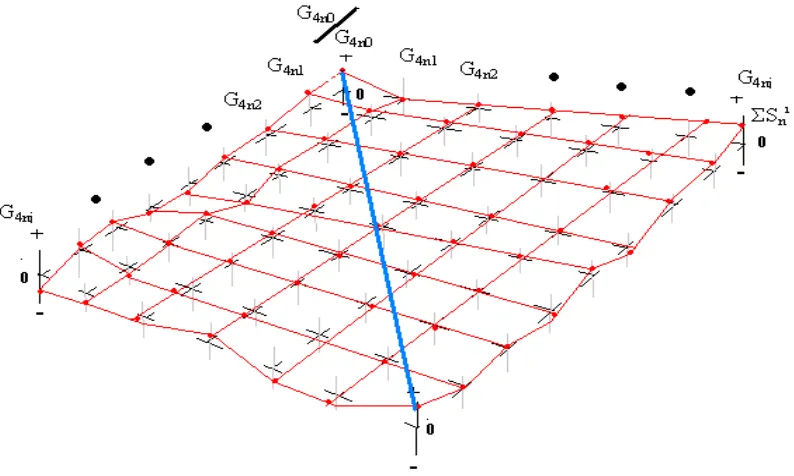
In this part of our model, we suggest to plot each production sector into four

different surfaces, to build each surface, we need to use such as reference all production

sub-sector outputs can be plotted on the surface mapping coordinate system, it can

facilitate to build each multi-dimensional surface for each production sector. After we

plot each production sub-sector, we proceed to join all production sub-sectors by strait

lines from the same production sector until we are available to build a single surface. The

main idea to build the four multi-dimensional surfaces is to observe the behavior of the

exchange of all production sub-sectors “i” by the exchange of a large number of

that in the center part of each surface is equal to 0. The reason is that the same sub-sector

cannot sell and buy the same commodity by itself (See Figure 1).

Figure 1: A Multi-dimensional Surface by Production Sector

The input-output dimensional analysis request the application of the

multi-dimensional partial differentiation (See Annex) to observe the changes of two periods of

time between the final time (t+1) and the initial time (t). Also in this part of the model,

we suggest the application of the economic modeling in real time “☼” (Ruiz, 2009) that

consist in successive application of differentiations to observe the changes into the four

production sectors simultaneously (See Expression 10). And also we suggest to apply the

inter-link of all production sub-sectors based on the application of the inter-link

coordinate axis condition that is represented by “╦”.

(10) ☼ΣS1i ≡ ΣS1’ = δƒ’ (S1)t / δ (S1)t+1d’S1 ╦ ΣS1’’= δƒ’’(S1)t/δ (S1)t+1 d2S1 ╦ ΣS1∞ = δ

ƒ∞(S1) / δ (S1)t+1 d∞S1

☼ΣS2i ≡ ΣS2’ = δƒ’ (S2)t / δ (S2)t+1d’S2 ╦ ΣS2’’= δƒ’’(S2)t/δ (S2)t+1 d2S2 ╦ ΣS2∞ = δƒ∞ (S2) / δ (S2)t+1 d∞S2

☼ΣS3i ≡ ΣS3’ = δƒ’ (S3)t / δ (S3)t+1d’S3 ╦ ΣS3’’= δƒ’’(S3)t/δ (S3)t+1 d2S3 ╦ ΣS3∞ = δƒ∞ (S3) / δ (S3)t+1 d∞S3

However, the construction and the final analysis of the input-output multi-dimensional

analysis consist in plot all multi-dimensional partial differentiations from each production

sector: agriculture, light industry, heavy industry and services (See Expression 11) on the

four dimensional physical space coordinate system. (See Ruiz, 2008.a.). In fact, to join

the four production sectors into the same graphical modeling, we suggest inter-link the

four production sectors based on the application of the inter-link of the general coordinate

condition that is represented by “╬”.

(11) GDP-Surface ≡ ☼S* ≡ ☼ΣS1i ╬ ☼ΣS2i ╬ ☼ΣS3i╬ ☼ΣS4i

The final output of the result input-output multi-dimensional analysis, we are

calling “GDP-Surface”. It is depend on the final position that the GDP-surface shows into

the four dimensional physical space coordinate system. We have four possible results

(See Expression 12, 13, 14 and 15) to analyze the behavior of the GDP according to the

speed of exchange of goods and services (economic activity) by production sector and

production sub-sectors.

(12) ☼S* ≡ ☼ +ΣS1i ╬ ☼ +ΣS2i ╬ ☼ +ΣS3i╬ ☼ +ΣS4i

{if +☼S* ∩ R+then the surface ≡ Economic Growth Synchronized}

(13) ☼S* = 0 ≡ ☼ ΣS1i = 0 ╬ ☼ ΣS2i = 0 ╬ ☼ ΣS3i= 0 ╬ ☼ ΣS4i = 0

{if ☼S* ∩ 0 then the surface ≡ General Economic Stagnation}

(14) ☼±S* ≡ ☼ ±ΣS1i ╬ ☼ ±ΣS2i ╬ ☼ ±ΣS3i╬ ☼ ±ΣS4i

{if ☼S* ∩ R+/-then the surface ≡ Irregular Economic Growth}

(15) ☼-S* ≡ ☼ -ΣS1i ╬ ☼ -ΣS2i ╬ ☼ -ΣS3i╬ ☼ -ΣS4i

Figure 2: I-O Multi-dimensional Graphical Analysis

3. Conclusion

We can observe that the input-output multi-dimensional analysis is available to catch up

the interaction of a large number of commodities exchange among different production

sub-sectors in the same production sector, in the same model also is possible to observe

the exchange among the four productions sectors (agriculture, light industry, heavy

industry and services sector) by the application of multi-dimensional partial

differentiations on complex group of functions that they are interacting in the same

mathematical and graphical modeling. Finally, the contribution of Professor Leontief was

great, but not enough to explain the behavior of the dynamic economy behaviors in our

times.

4. References

Ruiz Estrada, M. A. (2007.a). “Econographicology”, International Journal of Economics

Research (IJER), Vol 4-1. pp. 93-104.

Ruiz Estrada, M.A., Nagaraj, S. and Yap, S.F. (2007.b). “Beyond the Ceteris Paribus

Assumption: Modeling Demand and Supply Assuming Omnia Mobilis”. FEA-Working

Paper No.2007-9, pp.1-15.

Ruiz Estrada, M.A., (2009). “Economic Modeling in real Time?”. FEA-Working Paper No.2009-11, pp.1-15.

Leontief, W. (1951). The Structural of America Economy 1919-1939, Second Edition

Input Output Economic. Oxford University Press.

Leontief, W. (1951). The Structural of America Economy 1919-1939, Second Edition

Input Output Economic. Oxford University Press.

Annex

(1) dyij/dxij= 0 or ƒ’(xij) = 0

(2) d/dxij = nxn-1ij or ƒ’(xij) = nxn-1ij

(3) d/dcxij = cnxn-1ij or ƒ’(xij) = cnxn-1ij

(4) d/dxij[αij(xij) ± θij(xij) ±…±.λij(xij)] = d/dxij α(xij) ± d/dij θij(xij) ±…±.λij(xij)

or α’(xij) ± θ’(xij) ±…±.λ’(xij)

(5) d/dxij[αij(xij) θij(xij) … λij(xij)] = α(xij) d/dxij + θij(xij) +…+ .λij(xij)

α(xij) + θij(xij) d/dxij+…+ .λij(xij)

α(xij) + θij(xij) +…+ .λij(xij) d/dxij . . .

(6) d/dxij[αij(xij)/θij(xij)…λij(xij)]=α(xij) d/dxij+θij(xij)+…+λij(xij)/ [θij(xij) +…+ λij(xij)]2

d/dxij[θij(xij)/αij(xij)…λij(xij)]=α(xij)+θij(xij)d/dxij+…+λij(xij)/[αij(xij)+…+ λij(xij)]2

d/dxij[λij(xij)/αij(xij)…θij(xij)]=α(xij)+θij(xij)+…+λij(xij)d/dxij/[αij(xij)+…+ θij(xij)]2

(7) d/dx0j[α0j’(x0j) ╦ θ0j’(x0j) ╦ … ╦ λ0j’(x0j)]…

d/dx1j[α1j’(x1j) ╦ θ1j’(x1j) ╦ … ╦ λ1j’(x1j)]…

d/dx∞j[α∞j’(x∞j) ╦ θ∞j’(x∞j) ╦ … ╦ λ∞j’(x∞j)]…

(8) d/dx0j[α0j’(x0j) ╦ θ0j’(x0j) ╦ … ╦ λ0j’(x0j)] ╬

d/dx1j[α1j’(x1j) ╦ θ1j’(x1j) ╦ … ╦ λ1j’(x1j)] ╬