Vibration Control Using Heat Actuators

http://dx.doi.org/10.4236/wjm.2016.68018

Vibration Control Using Heat Actuators

Ilhan Tuzcu

Department of Mechanical Engineering, California State University, Sacramento, CA, USA

Received 3 July 2016; accepted 1 August 2016; published 4 August 2016

Copyright © 2016 by author and Scientific Research Publishing Inc.

This work is licensed under the Creative Commons Attribution International License (CC BY). http://creativecommons.org/licenses/by/4.0/

Abstract

This paper focuses on theoretical investigation of active vibration control of a cantilever beam us-ing heat actuation. The actuator is a thin metal bar rigidly bonded to the beam on one face and subject to heat input on the opposite face. The actuator then works like a piezoelectric actuator, and expands and contracts in response to applied heat. We assume that the actuator is insulated so that no heat is transferred to the beam, ensuring that the heat does not alter the beam’s thermal state. To avoid necessity of cooling, we consider two actuators working together at the same span- wise location, one on the upper and one on the lower face of the beam. Then, the beam can be bent up and down by applying heat to the lower and upper actuators, respectively. The governing equa-tions are partial differential equaequa-tions for one-dimensional heat conduction of the actuators and the bending vibration of the beam with attached actuators. For an approximate solution, Ray-leigh-Ritz method replaces the partial differential equations with a system of ordinary differential equations. A control model is obtained from a low-dimensional representation of the system, and used to design feedback control and observer by means of LQR and Kalman-Bucy filtering tech-niques. The control signal obtained is introduced into the plant model, a high-dimensional repre-sentation of the system, to mimic the true system as closely as possible. In a numerical application, the response of the beam to an initial excitation is simulated, which demonstrates that the heat actuators are in fact effective in active vibration control of the beam.

Keywords

Vibration Control, Heat Actuator, Temperature Control, Euler-Bernoulli Beam, Output Control

1. Introduction

Sensors do all measurements, but usually the states of the system cannot be measured directly. Hence, the ma-thematical model of the system is used to estimate all of the states based on the available measurements, pro-vided that the system is observable. The mathematical model is also used to compute the control signal to be in-puted to the actuator based on these estimates of the states. The actuator produces what is needed to affect the true system to suppress the vibration. This can be force, moment, strain, etc. The actuators widely used in vibra-tion control are hydraulic, pneumatic, and piezo-electric, with each having its own benefits and disadvantages depending on the specific applications in which they are used [1]. A special attention has been given to piezoe-lectric actuators in the recent years. These actuators are bonded on surfaces of structures at some discrete loca-tions to alter the local strain therein by the application of proper voltage signals to actuators [2].

Another type of actuation that has started receiving some attention in vibration control is simple heat. Consi-dering a structure initially at room temperature, an applied load causes temperature to vary over the body of the structure nonuniformly. Areas of the structure under tension are now cooler and areas under compression are hotter than the room temperature, creating a temperature gradient in the structure. This in turn causes a heat flow by conduction from hotter areas to cooler areas. Hence, a portion of the mechanical energy introduced to the structure is converted to heat through this process. Since the heat flow created is irreversible, the portion of the mechanical energy converted to heat is dissipated. This phenomenon is known as thermoelastic damping [3]. With this fact, question remains as to whether vibration in a structure can be suppressed by artificially introduc-ing a thermal gradient in the body by means of some external heat actuation. Some earlier studies had shown that, when applied properly, external heat actuation could in fact introduce significant amount of thermoelastic damping in structures [4]-[9].

Pioneering research by Edberg [4] considers control of vibration in a beam using a thermoelectric actuator, which has an ability to heat or cool the beam to produce a thermal gradient across the thickness of the beam. Experimental results reported in the paper show that with a simple lead compensation, damping ratio for the first vibrational mode of a cantilever beam is increased by more than nine times. Another work by Murozono and Sumi [5] also investigates active vibration control of a cantilever beam, but this time by heat input into the beam through the upper and lower surfaces, solely for creating a temperature gradient across the beam section. Foil strain gauges bonded on the surfaces are used as heat actuators. The heat input is through the upper or lower surface, depending on the direction of the gradient needed. Experiments reveal that the damping ratio for the first vibration mode is increased by about ten times. A computational study by Tuzcu et al. [6] considers a uni-form rod in longitudinal vibration and shows that control of both vibration and temperature can be achieved by heat input through thermoelectric actuators bonded on the lower and upper surfaces of the rod. Tuzcu and Gon-zalez-Rocha [7] extended the work of Tuzcu et al. [6] to a beam in bending. Both vibration and temperature are controlled simultaneously using thermoelectric actuators. Zhang et al. [8] proposes a vibration control of ther-mally induced vibration in space structures. Actuators are heaters bounded on the spacecraft structure at some optimal positions. Tuzcu et al. [9] explores the idea of using heat patches as actuators working in pairs on the upper and lower surfaces at some discrete spanwise locations of a uniform beam to simultaneously control vi-bration and temperature in the beam. A numerical example shows the presence of thermoelastic damping and demonstrates simultaneous control of elastic displacement and temperature gradient using a set of displacement measurements.

[image:3.595.187.445.87.294.2]

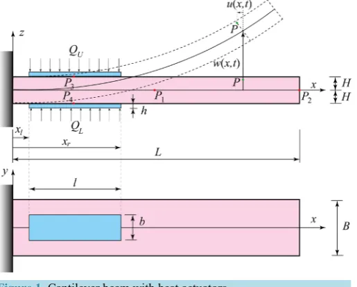
Figure 1. Cantilever beam with heat actuators.

2. Modeling

We will demonstrate our modeling and control approach on a cantilever beam, which is a fundamental element commonly encountered in structures. To make the presentation of our approach more clear and focus, we limit ourselves to a simple model by assuming the beam is uniform and there is only one pair of actuators, as shown in Figure 1. The beam is slender so that Euler-Bernoulli beam theory is valid. The upper and lower actuators are assumed to be rigidly bonded to the beam, which means the displacements of the beam and the actuators are equal at every point on the bonding surfaces. We define the displacement field in the beam as

(

, ,

)

w x, 0,

( )

,

u x z t z zw v w w x t

x ∂

= − = − = =

∂ (1)

where u v w, , are the displacement components in x y z, , -directions, respectively, and subscript x denotes a partial derivative with respect to x. Displacement components of a typical point P on the beam are illustrated in Figure 1. The beam’s left-end is fixed and its right-end is free so that w is subject to the boundary conditions:

( )

0, 0, x

( )

0, 0, xx

( )

, 0, xxx

( )

, 0

w t = w t = w L t = w L t = (2)

where each subscript x indicates a partial derivative with respect to x. Then, the strain components of the beam can be expressed as

2

2 , 0

xx u_x z _xw zwxx yy zz xy xz yz

ε =∂ = − ∂ = − ε =ε =ε =ε =ε =

∂ ∂ (3)

Since the ends of the actuators are free, the normal strains of the actuators will be constant at beam’s strains at its interface with the actuators [10], which means

( )

ε

xx L =Hwxx,

( )

ε

xx U = −Hwxx (4)

Assuming a linear stress-strain relation, we can express the only nonzero stress component in beam as

xx E xx Ezwxx

σ = ε = − (5) where E is the Young’s modulus of the beam. On the other hand, the normal stresses in the actuators are

( )

( )

(

)

( )

( )

(

)

xx L a xx L L a xx L

xx U a xx U U a xx U

E T E Hw T

E T E Hw T

σ ε α α

σ ε α α

 

= _ − _= −

 

= _ − _= − − (6)

where Ea is the Young’s modulus and α the coefficient of thermal expansion for the actuator material, and L

respectively. We assume the actuators are insulated on all faces except the ones that are subject to the heat inputs Q tL

( )

and Q tU

( )

, as shown in Figure 1. Because of these boundary conditions and assumption that

L

Q and QU are constant with x, we conclude that TL and TU are also constant with x, i.e. TL =T z tL

( )

,

and TU =T z tU

( )

, .

We approximate w, TU, as well as TL using the expansions

( )

,

( ) ( )

, U

( )

,

( ) ( )

U , L

( )

,

( ) ( )

L

w x t = Φ x q t T z t = Ψ z θ t T z t = Ψ −z θ t (7) where

( )

x φ1

( ) ( )

x φ2 x φm

( )

x ,

( )

z ψ1

( )

z ψ2

( )

z ψn

( )

z

Φ =_ _ Ψ =_ _ (8)

are the matrices consisting of m and n number of shape functions and

( )

( ) ( )

( )

( )

( )

( )

( )

( )

( )

( )

( )

1 2 1 2

1 2

, n ,

m U U U U

n

L L L L

t q t q t q t t t t t

t t t t

θ θ θ

θ θ θ

  =_ _ =_{ }   =   q θ

θ (9)

are the vectors of generalized coordinates for elastic displacement, and temperatures of the upper and lower actuators. Note that we use the same matrix of shape functions for the upper and lower actuators because we assume the actuators are identical and placed symmetrically about the x axis. We choose the shape functions

( )

, 1, 2, ,

i x i m

φ = to be the eigenfunctions of a uniform cantilever beam, which are given as

( )

sin sinh sin sinh

(

cos cosh

)

, 1, 2, ,

cos i cosh i

i i i i i

i i

L L

x x x x x i m

L L

β β

φ β β β β

β β

+

= − − − =

+ (10)

where βiL is the i-th βL solution of the characteristic equation cosβLcoshβ = −L 1. For example, the first

four solutions are β =1L 1.8751, β =2L 4.6941, β =3L 7.8548 and β =4L 10.9955.

Let us now express the total potential energy, which is the summation of potential energies of the beam and the lower and upper actuators:

( ) ( )

( ) ( )

(

)

(

( )

)

(

)(

)

2 2 2

0

2 2

1 _d 1 _d 1 _d

2 2 2

1 _d 1 _d 1 _{d d}

2 2 2

1 _d 1 _{d d}

2 2 L U r r l l r r l l

xx xx xx _L xx _L L xx _U xx _U U

V V V

L x x H

xx a a _x xx a _x xx _{H h} L

x x H h

a a _x xx a _x xx _H U

V V V

EI w x E A H w x E Hb w x T z

E A H w x E Hb w x T z

σ ε σ ε σ ε

α α − − + + = + + = + − + +

∫

∫

∫

∫

∫

∫

∫

∫

∫

∫

 (11)

where Aa=bh is the cross-sectional area of the each actuator, V is the volume of the beam, VL and VU are

the volumes of the actuators, and 2_d 2 3 3

I =

_∫

z A= BH is the area moment of inertia of the beam. Substituting Equation (7) into Equation (11), we rewrite the potential energy expression as

( ) ( )

( )

( )

T T

1

2 t K t t Ca t

= q q +q



θ

(12)

where

(

)(

)

( )

( )

( )

T 2

0

T

d 2 d ,

1 _{d d ,}

2

r l r

l

L x _T

xx xx a a _x xx xx

x H h

a a _x xx _H U L

K EI x E A H x

C E Hbα x + z θ t t t

= Φ Φ + Φ Φ

= Φ Ψ = −

∫

∫

∫

∫

θ θ

(13)

(

)

(

)

(

)

(

)

(

)

(

)

(

)

( )

( )

2 2 2 2 2 2

2 2 2 2 2 2 2 2 2

2 2 2 2 2 2 0 0

1 _d 1 _d 1 _d

2 2 2

1 _d 1 _d 1 _d

2 2 2

1 1 _{d d d}

2 3 1 2 L U L U r l

a L a U

V V V

x a x L a x U

V V V

L L x

x a a _x x

T

u w V u w V u w V

z w w V H w w V H w w V

mH w x m w x A H w w x

t M t

ρ ρ ρ

ρ ρ ρ

ρ = + + + + + = + + + + +   = _ + _+ +   =

∫

∫

∫

∫

∫

∫

∫

∫

∫

q q  (14)

where the mass matrix is

(

)

2 T T 2 T T

0

1 _{d 2 d d}

3

r l

L x

x x a a _x x x

M= _ mH Φ Φ + Φ Φm _ x+ ρ A H Φ Φ x+ Φ Φ x

 

∫

∫

(15)

where

ρ

is the density of the beam, m mass per unit length of the beam, and ρa density of the actuator

material.

Generalized force is obtained from the virtual work:

( ) ( )

T

( )

T T 0 , , d 0 , d

L L

W f x t w x t x f x t x

δ =

_∫

δ =δq

_∫

Φ =δq Q (16)

where f x t

( )

, is the applied lateral force per unit length, δw x t

( )

, virtual deflection of the beam, and

( )

( )

T

0 , d

L

t =

_∫

f x t Φ x

Q (17)

is the generalized force vector.

The equations of motion of the beam can be derived by means of Lagrange’s equations of motion, which can be written in the vector as

d dt

∂  ∂

− =

_∂  _∂  q q Q

  ₍₁₈₎

where   = − is the Lagrangian. Substituting Equations (12) and (14) into the Lagrangian, and the result into Equation (18), we get

a

Mq+Kq+Cθ =Q (19) Equation (19) governs the elastic deflection of the beam. Since this equation is coupled with the temperature difference

θ

, it must be solved simultaneously with the heat equations governing the temperatures in the upper and lower actuators. Hence, we next derive these heat equations.

The heat conduction in the upper actuator is described by the boundary-value problem defined by the following partial differential equation and boundary conditions:

2 2

1 TU TU

t z κ ∂ ∂ = ∂ ∂ 0 at U T

k z H

z ∂

= =

∂ (20)

at

U U

T Q

k z H h

z S

∂

= − +

∂

where

κ

is the thermal diffusivity, k the thermal conductivity, S bl= is the surface area of the upper face. We choose the shape functions ψi

( )

z i, =1, 2, , n as the eigenfunctions of the system defined by Equations (20) with QU =0, which are [11]

( )

cos

(

1 π

)

, 1, 2, ,

i z i z H_h i n

ψ = _ − − _ =

  (21)

the domain of the upper actuator, we get

(

H h T _d

)

(

H h T _d

)

U zz U

H z κ H z

+ +

Ψ Ψ = Ψ Ψ

∫

_θ

∫

_{θ (22)}

Similarly, substituting the second of Equations (7) into the boundary conditions, we get

( )

0,

(

)

U

z H U z H h U Q_kS

Ψ θ = Ψ + θ = (23)

Using the integration by parts, the second integral in Equation (22) can be written as

(

)

(

)

(

)

(

)

(

)

T T T

T T

d d

d

H h

H h H h

zz U z U z z U

H H H

H h U

z z U

H

z z

Q

H h z

kS

+

+ +

+

Ψ Ψ = Ψ Ψ − Ψ Ψ

= Ψ + − Ψ Ψ

∫

∫

∫

θ θ θ

θ (24)

Substituting Equation (24), Equation (22) can be rewritten in the compact form

U + U = QU

θ θ  (25) where

(

)

(

)

( )

T 2 T 2 T 1

2 0 0

0 1 0

d 2

0 0 1

0 0 0 0

0 1 0 0

π 0 0 4 0

d 2

0 0 0 1

1 1 1 H h H H h z z H n h z z h n H h kS kS κ κ κ κ + + −      

= Ψ Ψ =

             

= Ψ Ψ =

     ₋       ₋   

= Ψ + = _{ }

  −    

∫

∫

   (26)

Equation (25) completely describes the temperature in the upper actuator for prescribed heat input Q tU

( )

.

Note that by neglecting the thermoelasticity of the actuator, we assume the temperature is not affected by the elastic deformation of the beam. Equation (25) can be written in the state-space form

1 1

U = − − U + − QU

_{   }

θ θ (27)

which then leads to the following scalar equations for the individual generalized coordinates:

(

)

_{( )}

1 2 2 2 2 2 3 3 2 2 2 1 2 π 2

4 π 2

1 π ₁ 2

U U

U U U

U U U

n

n n

U U U

Q kSh Q kSh h Q kSh h n Q kSh h κ θ κ κ θ θ κ κ θ θ κ κ

θ θ −

Hence, the eigenvalues of the heat conduction are _{− −}

(

_{i 1}

)

2_κπ2 _h2 _{for i=1, 2, , n. We note that the} eigenvalue corresponding to i=1 is zero and all the remaining ones are negative real so that TU approaches

to a constant, instead of zero, as QU →0.

The heat conduction in the lower actuator is similarly described by the boundary-value problem

(

)

2 2 1 0 at at L L L L L T T t z T

k z H

z

T Q

k z H h

z S κ ∂ ₌ ∂ ∂ ∂ ∂ _{= = −} ∂ ∂ _{= = − +} ∂ (29)

Following the same steps, Equation (22) through Equation (24), we get

L+ L= QL

θ θ  (30) which governs the temperature in the lower actuator for prescribed heat input Q tL

( )

. The matrices , 

and  are as given in Equations (26). The scalar equations for the individual generalized coordinates for the lower actuator have the same forms as Equation (28). They can in fact be obtained by replacing the subscript U

by L in Equation (28). The eigenvalues are exactly same as the eigenvalues of the upper actuators.

2.1. Plant Model

Equations (19), (25) and (30) completely describe the motion of the uniform cantilever beam with the upper and lower actuators for prescribed inputs f x t

( )

, , Q tL

( )

and Q tU

( )

. We cast the system in the new first-order

form as

(

)

1 1 1 1

1 1 1

U U U

L L L

a U L

Q Q

M K M C M

− − − − − − − = − + = − + = = − − − + q s

s q Q

        θ θ θ θ θ θ (31)

which can be rewritten in the state-space form

A B

= +

x x u (32) where , U U L L Q Q           = _{=  }           x u q Q s θ θ (33)

are the state and input vectors, and

1 1

1 1

1 1 1 1

0 0 0 0 0

0 0 0 _, 0 0

0 0 0 0 0 0

0 0 0

a a

A B

I

M C M C M K M

− − − − − − − − −     ₋        =_{ } =_{ }     − −  −                (34)

are the coefficient matrices. Note that the dimensions of x, u, A, and B are 2

(

m n+

)

×1,

(

m+ ×2 1

)

,

(

) (

)

2 m n+ ×2 m n+ , and 2

(

m n+

) (

× m+2

)

, respectively.

We will call the state-space model of Equation (32) the plant model, which, in absence of an experimental model, will be used to simulate the behavior of the actual system and to test the performance of our control design. In order for this model to approximate the behavior of the actual system better, we will choose m and n

the other hand, will be based on a control model that uses a less number of shape functions, as explained next. Our objective in this paper is to control the deflection of the beam using Q tL

( )

and Q tU

( )

as the control

inputs. The challenge is that the control has to be done for positive values of Q tL

( )

and Q tU

( )

so that

cooling of the actuators is never necessary. This paper offers a novel approach to overcome this challenge. The beam’s deflection is governed by Equation (19) from which we note the deflection is actually affected by the difference θ =θU −θL. Subtracting Equation (30) from Equation (25), we get

Q

+ =

θ θ  (35) where Q Q= U −QL. Hence, for the control objective, Equation (35) is coupled with Equation (19) so that the

difference Q Q= U −QL can be used as the control input instead of the individual inputs QU and QL. The

control of the deflection will certainly require both negative and positive values of the input Q, which can be achieved by properly choosing the individual inputs QU and QL. In fact, to avoid unnecessary heat inputs into

the beam, we choose QU and QL as follows: If negative Q is required, we achieve it by choosing QU =0

and QL= −Q. Similarly, if positive Q is required, we choose QU =Q and QL=0.

2.2. Control Model

Control design must be as simple as possible for easy implementation and fast real-time computations. This in turn requires a low-order control model. To that end, we first note that the second integral of the expression for

a

C defined in Equation (13) has a matrix value

[

]

d 0 0

H h

H z h

+

Ψ =

∫

(36)

which clearly means the first column is the only non-zero column in Ca, which in turn means the only tem-

perature component appearing in the equation governing elastic deflection, Equation (19), is 1 1

1 U L

θ =θ −θ , and

not any of 2 2

2 U L

θ =θ −θ , , n n

n U L

θ =θ −θ . Hence, the control of the elastic deflection by applying heat input can be achieved only through θ1. For this reason, in the control model, we will choose n=1 and keep the governing equation for θ1 only. Then, the coupled system can be expressed in the state-space model as

c=Ac c+B uc c

x x (37) where

1 ,

c uc Q

θ    

=_{ } =

   

x q

s

(38)

are the control state vector and the control input, and

1 1

0 0 0

0 0 , 0

0 0

c c

a

kSh

A I B

M C M K

κ

− −

 

 

 

 

 

=_{  =  }

 

− − 

  _{ }

 

(39)

The dimensions of xc, uc, Ac and Bc in this case are

(

1 2+ m

)

×1, 1 1× ,

(

1 2+ m

) (

× +1 2m

)

, and

(

1 2+ m

)

×1, respectively. To keep the dimension even smaller, we will use an m for the control model several times smaller than for the plant model. Note that this model allows us to control not only the deflection in the beam, but also θ1, which is the most dominant temperature component among all θ1, ,θn.

3. Output Feedback Control Design

number of control input available is only one. The order of the control model can get very high depending on the chosen m. Linear Quadratic Regulator (LQR) seems to be one of the best design methods available for this type of systems. The LQR design method determines an optimal control gain matrix G so that the control input

( )

( )

c c

u t = −Gx t minimizes the quadratic performance measure

( )

( )

( )

( )

0

T T

1 _d

2

f

t

c c c c c c

t

J =

_∫

_x t Q x t +u t R u t _ t (40) where Qc is a real symmetric positive semidefinite matrix, Rc a real symmetric positive definite matrix, and

0

t and tf are the initial and the final times [12]. The LQR yields the control gain matrix as 1 T

c c c

G R B K₌ − ₍₄₁₎

where Kc is a real symmetric matrix satisfying the algebraic matrix Riccati equation

T 1 T ₀

c c c c c c c c c c

A K ₊K A Q K B R B K_{+ −} − _{= (42)}

The control design described above assumes that the state vector xc

( )

t is available for feedback since it

uses the input as u tc

( )

= −Gxc

( )

t . However, in reality, xc

( )

t must be estimated from the output y

( )

t of

the actual system, which includes a number of measurements of deflection and/or its rate on the beam. Then, the control input can be obtained from u tc

( )

= −Gxˆc

( )

t where xˆc

( )

t is the estimate of xc

( )

t . Using our

control model, the estimate xˆc

( )

t is obtained through an observer design whose dynamics is described by the

matrix differential equation

( )

( )

( )

( )

( )

ˆ_c t =A_{c c}ˆ t +B u t_{c c} + ∆_ t − ˆ t _

x x y y (43)

where ∆ is the observer gain matrix and ˆy

( )

t =C_{c c}xˆ

( )

t is the estimate of the actual output y

( )

t [12]. Using the Kalman-Bucy Filter, ∆ is obtained from T 1

c

C W−

∆ = Σ where W is the sensor noise intensity matrix and Σ is the solution of the algebraic matrix Riccati equation

T T 1 ₀

c c c c

A_{Σ + Σ}A _{+ − Σ}V C W C− _{Σ = (44)}

in which V is the state excitation noise intensity matrix.

We assume deflection measurements at the points P1 and P2 shown in Figure 1 are available as output signals. Since we use the plant model to approximate the actual system, the output of the plant can be written as

( )

1

( )

_{( )}

(

_{( )}

)

( )

2

2, ,

y t w L t

y t Cx t

y t w L t

   

=_{  }= _=

    (45)

where

(

)

( )

0 0 2 0

0 0 0

L C

L

 Φ 

=  _Φ 

  (46)

is the output matrix relating the actual state to the output. The estimate of the output, on the other hand, is written as

( )

1

( )

_{( )}

(

_{( )}

)

( )

2

ˆ ˆ 2,

ˆ ˆ , c c

y t w L t

y t C x t

y t w L t

   

=_{  }= _=

    (47)

where

(

)

( )

0 2 0

0 0

c

L C

L

 Φ 

=  _Φ 

  (48)

is the output matrix relating the estimated state to the estimated output.

Once Q t

( )

=Q tU

( )

−Q tL

( )

is obtained from u tc

( )

=Q t

( )

= −Gxˆc

( )

t , the individual Q tL

( )

and Q tU

( )

( )

( )

( )

( )

( )

( )

( )

( )

If 0, and 0

If 0, 0 and

U L

U L

Q t Q t Q t Q t

Q t Q t Q t Q t

≥ = =

< = = − (49)

4. Numerical Application

The modeling approach and the control design presented above will be numerically demonstrated for a uniform cantilever beam. We will use the same cantilever beam and the related parameters used in [9] so that we can compare the results from this paper directly to the ones from [9]. Physical parameters of the beam and the actuators are listed in Table 1. For most effective actuators, we choose xl =0 and xr =l so that the actuators

are closed to the root where the strain is high. As revealed in Table 1, the material of the beam is chosen to be steel. We choose steel also for the actuators because it has high Eaα , which makes the actuators more effective.

Using the values of the parameters listed in Table 1, we construct the matrices M, K and Ca using the ex-

pressions given in Equations (13) and (15). To give the reader an idea about the numerical forms of these matrices, we present them for some small number of m and n, namely m=2 and m=3:

1.1775 0.0275 0.2847 0.2087 0.0669 0 0

kg, kN m, N K

0.0275 0.6787 0.2087 3.9248 a 0.0477 0 0

M =_ _ K =_ _ C =_ _

      (50)

The matrices ,  and  are as given in Equation (26). A and B matrices given in (34) can be con- structed by using the numerical forms of the submatrices:

1 1

1 2 1 2

1

0 0 0 2

0 509.27 0 K s, 0.0717 1 K s W

0 0 2037.1 1

0.0552 0 0 234.88 42.379

m s K , 1 s ,

0.0680 0 0 42.379 5781.1

0.8501 0.0344 1 kg 0.0344 1.4748

a

M C M K

M

− −

− −

−

   

   

=_{ } = _{ }− ⋅

   

   

   

=_{ } ⋅ =_{ }

   

−

 

= ₋ 

 

   

(51)

To demonstrate the simulation of the closed-loop system, we choose m=7 and n=10 for the plant model and m=3 and n=1 for the control model so that A is 34 34× , B 34 9× , C 2 34× , Ac 7 7× , Bc 7 1× ,

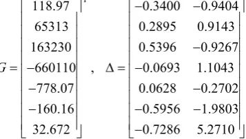
and Cc 2 7× . For the control and observer designs, we choose the following design parameters:

[

]

[

]

7

2 10 , diag 0.001,1,1,1,1,1,1 , diag 1000,1,1,1,1,1,1 ,

c c

R ₌ − Q ₌ V ₌ W I₌

(52) where “diag” means diagonal matrix and I2 is 2 2× identity matrix. Then, the control and observer gain matrices are computed to be

T

118.97 0.3400 0.9404

65313 0.2895 0.9143

163230 0.5396 0.9267

,

660110 0.0693 1.1043

778.07 0.0628 0.2702

160.16 0.5956 1.9803

32.672 0.7286 5.2710

G

− −

   

   

   

   − 

   

=_− _ ∆ =_− _

₋   ₋ 

   

− − −

   

  ₋ 

   

(53)

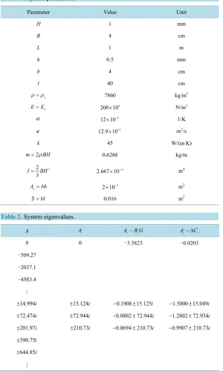
[image:10.595.217.396.530.631.2]

[image:11.595.156.475.93.622.2]

Table 1. Physical parameters.

Parameter Value Unit

H 1 mm

B 4 cm

L 1 m

h 0.5 mm

b 4 cm

l 40 cm

a

ρ ρ= 7860 kg/m3

a

E E= _{200 10×} 9 _N/m2

α _{12 10×} −6 _1/K

κ _{12.9 10×} −6 _m2_/s

k 45 W/(m⋅K)

2

m= ρBH 0.6288 kg/m

3 2 3

I= BH _{2.667 10×} −11 _m4

a

A =bh _{2 10×} −5 _m2

S bl= 0.016 m2

Table 2. System eigenvalues.

A Ac A B Gc− c Ac− ∆Cc

0 0 −3.5823 −0.0203

−509.27

−2037.1

−4583.4

14.994i

± ±15.124i −0.1908 15.125± i −1.5000 15.049± i

72.474i

± ±72.944i −0.0802 72.944± i −1.2802 72.934± i

201.97i

± ±210.73i −0.0694 210.73± i −0.9907 210.73± i

390.75i

±

644.85i

±

will be answered by the simulation of the closed-loop plant.

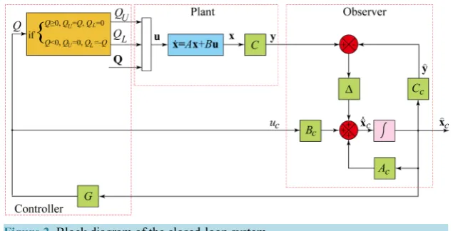
Block diagram shown in Figure 2 completely describes how the control of the plant is implemented. We will test the performance of our control design by simulating the response of the closed-loop plant to the same initial conditions used in [9], namely

( )

1

_{( )}

( )

( )

1

,0 20 x mm, ,0 0

w x w x

L

φ φ

[image:12.595.154.472.82.244.2]

Figure 2. Block diagram of the closed-loop system.

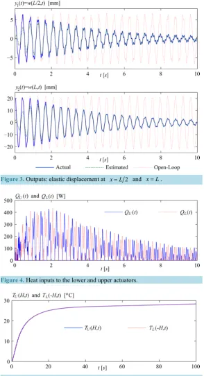
so that the beam is initially at rest in the shape of φ1

( )

x with 20 mm tip displacement. Time histories of open- loop, actual, and estimated outputs, namely elastic displacement at x L= 2 and x L= are plotted in Figure 3. Comparing Figure 3 to the last of Figure 2 of [9], we conclude that the damping achieved in the present paper is about the same as that of [9]; in both, tip displacement reduces to 5 mm in approximately 16 cycles.

Figure 4 shows the heat inputs to the lower and upper actuators needed to achieve this damping. Considering that the amplitude of the vibration in this numerical example is high, these heat inputs seem to be reasonable. Even though [9] uses heat actuators in two spanwise locations, the required heat inputs are quite similar to those of this paper.

In this paper, we assume each actuator is insulated in all faces except the face that is subject to the heat, including the faces normal to x and y axes. This assumption clearly means the temperatures everywhere in the actuators increase monotonically until the heat inputs are ceased after vibration amplitude reduces to a desired value. As an example, temperatures TL

(

−H t,

)

and T H tU

(

,

)

versus t for 100 s are shown in Figure 5, from

which we read TL

(

−H,100

)

=28.32 C˚ and T HU

(

,100

)

=28.32 C˚ . Since the heat is confined to a small

volume in the actuators, the temperatures get very high, but still much less than the material of the actuators can tolerate. To prevent the temperatures in the actuators to get very high values, some sort of cooling, such as thermoelectric cooling, can be used to cool the actuators. In that case, cooling must be introduced into the control design as a disturbance. Contrary to the actuators, no temperature changes occur in the cantilever beam. In [9], since the heat is directly applied to the beam itself, which has a much larger volume than the actuators of this paper, the temperature increase in the beam is limited to few degrees.

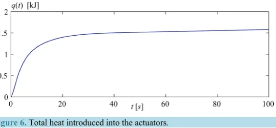
We can also compare the total heat injected into the volumes in the two papers. we compute the total heat input to the actuators within t seconds as the integral of total heat rate:

( )

₀t _L

( )

_U

( )

d

q t =

_∫

_Q ξ +Q ξ _ ξ (55)

( )

q t versus t is plotted for 100 seconds in Figure 6, from which we read the total heat input to the actuators in 100 s as q

( )

100 1.581 kJ= . On the other hand, in [9], q

( )

100 =2.555 kJ, which is much larger than the heat input in the present paper.

5. Conclusions

[image:13.595.166.461.85.628.2] [image:13.595.175.457.87.344.2]

Figure 3. Outputs: elastic displacement at x L= 2 and x L= .

Figure 4. Heat inputs to the lower and upper actuators.

Figure 5.Actuator temperatures.

[image:14.595.174.457.84.215.2]

Figure 6.Total heat introduced into the actuators.

the equation governing the temperature in each actuator. We also assume the temperatures of the actuators are not affected by the elastic motion. The governing equations are a set of three partial differential equations, each of which has an infinite dimension. For an approximate solution, we use Rayleigh-Ritz method to replace the partial differential equations with a desired number of ordinary differential equations, obtaining a finite, but oth-erwise high-dimensional system. The higher the dimension, the more accurate the model is.

We obtain the plant model by using a high-dimensional representation of the system so that it can be repre- sented as accurately as possible. On the other hand, we obtain the control model by using a low-dimensional re-presentation of the system so that estimates of the states as well as control inputs can easily be computed in real time. Since we do not have an experimental model, we use the plant model to mimic the true system as closely as possible, which is the reason to choose a high dimensional model. The control model is used to design feed-back control and observer by means of LQR and Kalman-Bucy filtering techniques. The observer design is based on only two displacement measurements, one in the middle and one at the free end of the beam.

In a numerical application, control signal is computed using the control and observer gains based on the con-trol model, and inputted into the plant. Then, the response of the beam to an initial excitation is simulated. The numerical simulation demonstrates that the actuators are in fact effective in active vibration control of the beam. The results obtained are comparable to some of the results of [9]. For comparison reason, the feedback control is designed so that approximately the same damping factor as that of [9] is achieved. However, we show that the total heat input needed to achieve this damping is much smaller than that of [9], from which we conclude that the actuators of this paper are more effective than those of [9].

For simplicity of the models, we assume that each actuator is insulated in all faces except the face it is subject to heat. With this assumption, the heat conduction is one-dimensional (only in z-direction), and also we do not have to make assumptions about the convection and/or radiation heat transfer from the faces normal to x and y

axes to outside. However, in real-life applications, this assumption is hard to enforce and it must be relaxed. Our future work will aim to make design alterations to relax this assumption to make the work more applicable to real-life situations.

Acknowledgements

The author thanks the editor and the referee for their comments.

Dedication

This paper is dedicated to the memory of Prof. Leonard Meirovitch.

References

[1] Huber, J.E., Fleck, N.A. and Ashby, M.F. (1997) The Selection of Mechanical Actuators Based on Performance Indic-es. Proceedings of the Royal Society A, 453. 2185-2205. http://dx.doi.org/10.1098/rspa.1997.0117

[2] Jalili, N. (2010) Piezoelectric-Based Vibration Control: From Macro to Micro/Nano Scale Systems. Springer, New York.

[3] Nowinski, J.L. (1978) Theory of Thermoelasticity with Applications. Sijthoff & Noordhoff International Publishers.

[4] Edberg, D.L. (1987) Control of Flexible Structures by Applied Thermal Gradients. AIAA Journal, 25, 877-883.

http://dx.doi.org/10.2514/3.9715

[5] Murozono, M. and Sumi, S. (1994) Active Vibration Control of a Flexible Cantilever Beam by Applying Thermal Bending Moment. Journal of Intelligent Material Systems and Structures, 5, 21-29.

http://dx.doi.org/10.1177/1045389X9400500103

[6] Tuzcu, I., Asmatulu, R. and Hasanyan, D. (2003) Control of the Vibration and Temperature in a Thermoelastic Rod. Proceedings of 5th International Congress on Thermal Stresses and Related Topics, Blacksburg, 8-11 June 2003. [7] Tuzcu, I. and Gonzalez-Rocha, J. (2013) Modeling and Control of Thermoelastic Beam. Proceedings of the ASME

Dynamic Systems and Control Conference, Palo Alto, 21-23 October 2013, V001T06A004.

http://dx.doi.org/10.1115/dscc2013-4025

[8] Zhang, J., Xiang, Z. and Liu, Y. (2014) Control of the Thermally Induced Vibration of Space Structures by Using Heaters. Journal of Spacecraft and Rockets, 51, 1454-1463. http://dx.doi.org/10.2514/1.A32601

[9] Tuzcu, I., Moua, J.K. and Olivares, J.G. (2016) Control of a Thermoelastic Beam Using Heat Actuation. Journal of Vibration and Control, in press. http://dx.doi.org/10.1177/1077546316629251

[10] Crawley, E.F. and de Luis, J. (1987) Use of Piezoelectric Actuators as Elements of Intelligent Structures. AIAA Journal, 25, 1373-1385. http://dx.doi.org/10.2514/3.9792

[11] Özişik, M.N. (1980) Heat Conduction. John Wiley & Sons, Inc., New York.

[12] Meirovitch, L. (1990) Dynamics and Control of Structures. John Wiley & Sons, New York.

Submit or recommend next manuscript to SCIRP and we will provide best service for you: Accepting pre-submission inquiries through Email, Facebook, LinkedIn, Twitter, etc.

A wide selection of journals (inclusive of 9 subjects, more than 200 journals) Providing 24-hour high-quality service

User-friendly online submission system Fair and swift peer-review system

Efficient typesetting and proofreading procedure

Display of the result of downloads and visits, as well as the number of cited articles Maximum dissemination of your research work